Adaptive Sliding Mode Trajectory Tracking Control for Unmanned Surface Vehicle with Modeling Uncertainties and Input Saturation

Abstract

In the presence of modeling uncertainties and input saturation, this paper proposes a practical adaptive sliding mode control scheme for an underactuated unmanned surface vehicle (USV) using neural network, auxiliary dynamic system, sliding mode control and backstepping technique. First, the radial basis function neural network with minimum learning parameter method (MLP) is constructed to online approximate the uncertain system dynamics, which uses single parameter instead of all weights online learning, leading to a reduction in the computational burdens. Then a hyperbolic tangent function is adopted to reduce the chattering phenomenon due to the sliding mode surface. Meanwhile, the auxiliary dynamic system and the adaptive technology are employed to handle input saturation and unknown disturbances, respectively. In addition, a neural shunting model is introduced to eliminate the “explosion of complexity” problem caused by the backstepping method for virtual control derivation. The stability of the closed-loop system is guaranteed by the Lyapunov stability theory. Finally, simulations are provided to validate the effectiveness of the proposed control scheme.

1. Introduction

With the development of marine technology, unmanned surface vehicle (USV) has attracted great attention in the field of ocean. This is mainly due to its advantages of being fast, small volume, low cost, and the ability of autonomous navigation. Based on the above advantages, USV has been widely used in many applications, such as oil and gas exploration, ocean surveillance, search, rescue and military [1,2,3,4,5]. However, the performance of the system is significantly decreased due to the influence of external factors, particularly in the presence of the uncertain system dynamics and external disturbances. Therefore, it is very important to design a controller with the anti-interference capability and higher precision for USV.

In recent years, trajectory tracking has been a hot topic of research due to its practical importance. Trajectory tracking is defined as a vessel being required to follow a reference path with spatial and temporal constraint, namely, a reference path with an associated time law [6,7]. At present, a variety of control schemes associated with trajectory tracking control design for surface vessel have been developed in literature. Global smooth controllers are designed in [8], which achieve the practical stabilization of arbitrary reference trajectories. In [9], a state feedback based backstepping control strategy is proposed, which can enhance the steady state performance and control precision of USV. However, in actual voyage, the model of USV may change due to external disturbances and other factors. In order to overcome this difficulty, an adaptive tracking controller based on backstepping and neural network is developed in [10], in which neural network is hired to handle the unknown dynamics. Based on the sliding mode control and the minimum learning parameter (MLP) technique, an adaptive tracking control scheme is proposed in [11], where dynamical uncertainty and time-varying ocean disturbances are centrally compensated by employing neural network MLP. In addition, for the trajectory tracking problem of the underactuated USV, the biggest challenge is that the number of actuators is less than the degree of freedom, which increases the design difficulty of the controller. Some previous solutions have been published in [12,13]. A trajectory tracking controller is applied to underactuated surface ships in [12], where the model is represented by numerical methods. Its main advantage is that the calculation of control actions are obtained, solving a system of linear equations. In [13], three modified dynamic inversion methods are proposed to solve the tracking control problem of the underactuated ship, which can remove some of its inherent limitations, making it applicable to a wide variety of underactuated systems. Based on the above analysis, there are still many problems to be solved for tracking control of the underactuated USV.

Considering the ship motion control, several authors have contributed a set of novel ideas and strategies. In [14], a robust adaptive control scheme based on modified function projective synchronization is proposed, which can be used in various types of synchronization. Based on dynamic surface control and neural network techniques, a concise adaptive neural network control scheme is proposed in [15]. Its advantage is that the control law has a concise form and is easy to implement, but its disadvantage is that it does not take into account control input hysteresis nonlinearity. In [16], an adaptive fuzzy optimal control method is addressed, which not only guarantees the stability of the system, but also achieves the optimal control performance. With the consideration of robustness, sliding mode control [17] is a successful robust control algorithm, which has been widely used in ship motion control [18,19,20,21], especially in practical engineering. Based on backstepping technique and adaptive dynamical sliding control method, a novel adaptive algorithm is proposed to deal with unknown disturbances and system uncertainties in [22]. However, there are too many assumptions about the first derivative of the disturbance and the existence of the thruster. The paper [23] develops a sliding mode controller based on proportional integral (PI) sliding mode control, in which an adaptive term is designed to effectively solve the problem of system chattering. The main drawback is that an integral term may cause the reduced stability margin due to phase lag [24]. In order to further simplify the model and avoid the underactuation problem, a novel methodology is developed in [25]. Unfortunately, the tracking accuracy is low due to the use of a simple control law that achieves asymptotic path following. Although there are various problems, the sliding mode control is still an effective control algorithm to deal with nonlinear control problems. From a practical perspective, the input saturation is unavoidable due to physical constraints in propulsion systems. If the input saturation is neglected in control design, it will lead to the instability of the system and even the collapse of the control system. In the presence of the input saturation, an adaptive impedance controller is developed for an n-link robotic manipulator in [26], where an auxiliary system is adopted to handle the input saturation. The paper [27] designs a novel robust adaptive ship trajectory tracking control law for surface ships, in which the input saturation is approximated using a Gaussian error function. Hence, the influence of input saturation should be considered in control design.

Based on the discussion above, considering actuator saturation and modeling uncertainties, an adaptive sliding mode control approach is developed by employing sliding mode control, the MLP technique, backstepping method and the auxiliary system, which accurately makes the underactuated USV track a desired trajectory. The primary contributions of this paper are summarized as follows:

(1)

A novel adaptive control strategy based on sliding mode control and backstepping method is presented for the underactuated USV, in which the hyperbolic tangent function and the neural shunting model are adopted to eliminate the chattering phenomenon and the “explosion of complexity” problem of the system, respectively. Comparing with the previous work [28], it is more effective to implement the control scheme in real practice.

(2)

Taking full account of the practical engineering, the input saturation is handled by designing an auxiliary system. The MLP technique and the adaptive technology are used to deal with unmodeled dynamics and unknown disturbance bounds, respectively, where the norm of all the weights is estimated instead of estimating each element. Only two weight-norm related parameters are required to be updated in the control law.

This brief is organized as follows. In Section 2, problem formulation and preliminaries are presented. Section 3 illustrates a novel adaptive control scheme for the underactuated USV. The stability analysis of the whole system is given in Section 4. The simulation results to illustrate the proposed controller are shown in Section 5. Finally, Section 6 concludes this paper.

2. Problem Formulation and Preliminaries

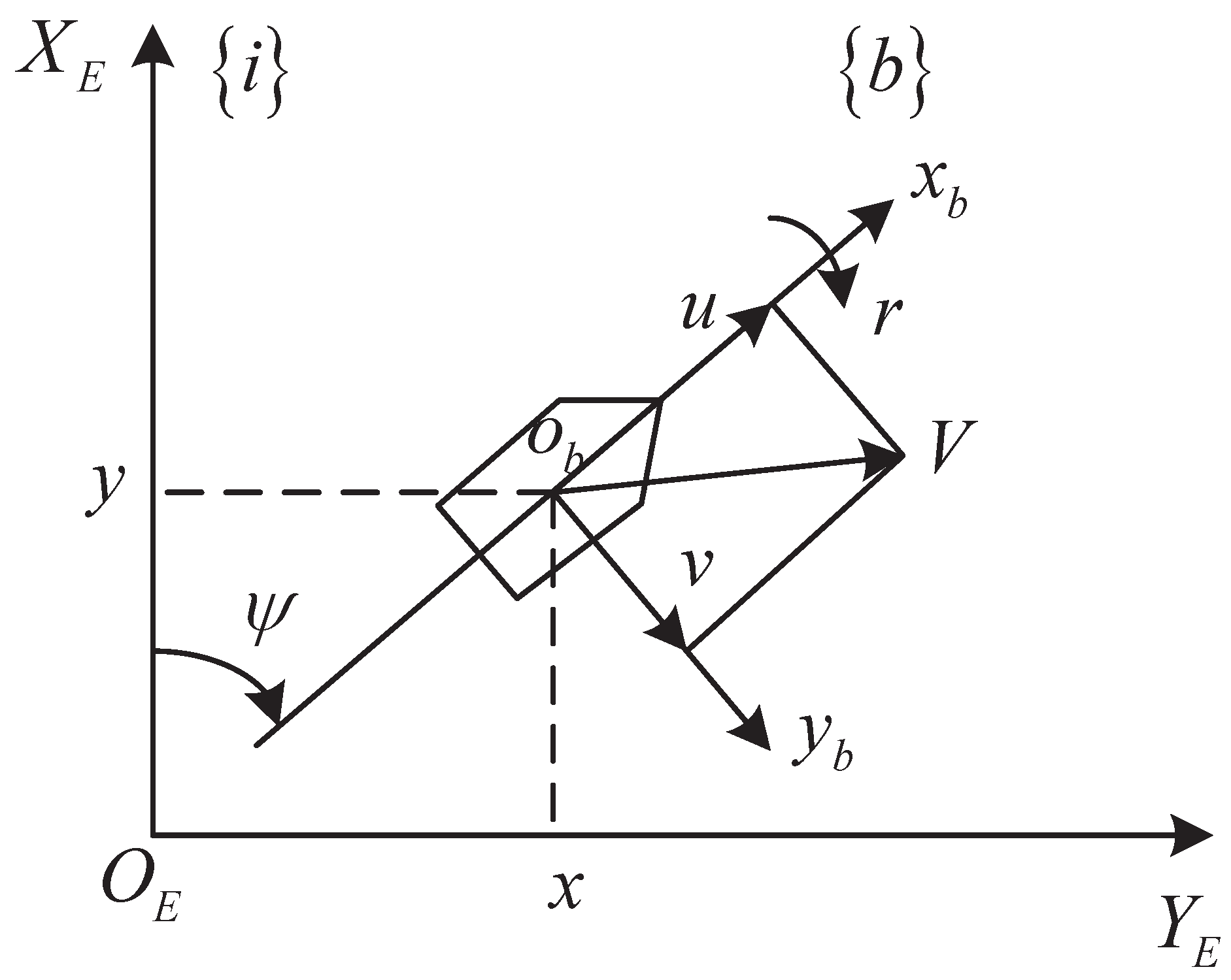
2.1. Problem Formulation

In this section, two reference frames are considered to study the USV model. The horizontal plane motion of USV is described by the position and orientation, namely, neglecting roll, pitch and heave, as illustrated in Figure 1, in which $X_E{O}_E{Y}_E$ is the earth-fixed inertial frame $\left\{i\right\}$ and $x_b{o}_b{y}_b$ is the body-fixed frame $\left\{b\right\}$. The position $\left(x,y\right)$ in $\left\{i\right\}$ represents the actual location of USV, and $\psi \in \left(0,2\pi \right)$ is course angle. In addition, u, v and r denote the surge velocity, the sway velocity and the yaw rate of USV, respectively.

Based on the above analysis, the kinematics and dynamics mathematical model of the three degrees of freedom [29] can be described as

$$\begin{array}{c}\hfill \begin{array}{c}\dot{\eta }=J\left(\psi \right)\upsilon \hfill \\ M\dot{\upsilon }+C\left(\upsilon \right)\upsilon +D\upsilon =\tau +d\left(t\right)\hfill \end{array}\end{array}$$

(1)

where $\eta ={\left[x,y,\psi \right]}^T$, $\upsilon ={\left[u,v,r\right]}^T$, $J\left(\psi \right)=\left[\begin{array}{ccc}cos\psi & -sin\psi & 0\\ sin\psi & cos\psi & 0\\ 0& 0& 1\end{array}\right]$ is the rotation matrix from $\left\{b\right\}$ to $\left\{i\right\}$; $M=\left[\begin{array}{ccc}{m}_{11}& 0& 0\\ 0& m_{22}& m_{23}\\ 0& m_{32}& m_{33}\end{array}\right]$ is the inertial matrix, and $C\left(\upsilon \right)\in R^{3\times 3}$ is the matrix of Coriolis and centripetal terms; $D=\left[\begin{array}{ccc}{d}_{11}& 0& 0\\ 0& d_{22}& d_{23}\\ 0& d_{32}& d_{33}\end{array}\right]$ is the damping matrix; $\tau ={\left[{\tau }_u,0,{\tau }_r\right]}^T$, in which ${\tau }_u$ and ${\tau }_r$ denote the surge force and yaw moment, respectively. In practice, the amplitude and change rate of the equivalent control resultant force and moment are possibly constrained due to physical limitations of the propulsion system, which can be described as

$$\begin{array}{c}\hfill {\tau }_j=\left\{\begin{array}{c}{\tau }_{jmax},if{\tau }_{cj}>{\tau }_{jmax}\hfill \\ {\tau }_{cj},if{\tau }_{jmin}<{\tau }_{cj}<{\tau }_{jmax}\hfill \\ {\tau }_{jmin},if{\tau }_{cj}<{\tau }_{jmin}\hfill \end{array}\right.\end{array}$$

(2)

where ${\tau }_{jmax}$ and ${\tau }_{jmin}$ $\left(j=u,r\right)$ are the maximum and the minimum control forces or moments, ${\tau }_{cj}$ is the commanded control calculated by adaptive sliding mode controller. In addition, $d\left(t\right)={\left[d_u,d_v,d_r\right]}^T$ represent unknown time-varying ocean disturbances.

Assume that USV is symmetrical, the origin of the attached coordinate system and the barycentre of USV are coincident [10,30,31]. (1) can be rewritten as the following state-space equations

$$\begin{array}{c}\hfill \left\{\begin{array}{c}\dot{x}=ucos\psi -vsin\psi \hfill \\ \dot{y}=usin\psi +vcos\psi \hfill \\ \dot{\psi }=r\hfill \end{array}\right.\end{array}$$

(3)

$$\begin{array}{c}\hfill \left\{\begin{array}{c}\dot{u}=f_u+\frac{\Delta f_u}{m_{11}}+\frac{{\tau }_u}{m_{11}}+\frac{d_u}{m_{11}}\hfill \\ \dot{v}=f_v+\frac{\Delta f_v}{m_{22}}+\frac{d_v}{m_{22}}\hfill \\ \dot{r}=f_r+\frac{\Delta f_r}{m_{33}}+\frac{{\tau }_r}{m_{33}}+\frac{d_r}{m_{33}}\hfill \end{array}\right.\end{array}$$

(4)

where $f_u=\frac{m_{22}}{m_{11}}vr-\frac{d_{11}}{m_{11}}u$, $f_v=-\frac{m_{11}}{m_{22}}ur-\frac{d_{22}}{m_{22}}v$, $f_r=\frac{\left(m_{11}-m_{22}\right)}{m_{33}}ur-\frac{d_{33}}{m_{33}}r$, in which $\Delta f={\left[\Delta f_u,\Delta f_v,\Delta f_r\right]}^T$ represents the uncertain system dynamics.

Assumption 1.

The reference trajectory $\left(x_d,y_d\right)$ is smooth and differentiable, $x_d$, ${\dot{x}}_d$, $y_d$ and ${\dot{y}}_d$ are all bounded.

Assumption 2.

[32] The external disturbances $d_i\left(i=u,v,r\right)$ are bounded by $\left|d_i\right|\le d_i^{*}$, where $d_i^{*}$ are unknown positive constants.

Control objective: Considering model uncertainty and input saturation, the USV accurately tracks the reference path $\left(x_d,y_d\right)$ according to the design of the surge force ${\tau }_u$ and the yaw moment ${\tau }_r$. All state variables are proved to be semi-globally uniformly ultimately bounded.

2.2. Neural Network MLP Method

In control engineering, neural networks are used to approximate unknown uncertainties [33,34], especially radial basis function (RBF) neural network, which has a strong self-learning ability. The RBF neural network consisting of input layer, hidden layer and output layer, which can be written as

$$\begin{array}{c}\hfill f_n\left(z\right)=W_n^T\mathsf{\Theta }\left(z\right)+{\epsilon }_n\end{array}$$

(5)

where $z={\left[u,v,r\right]}^T$ and $f_n\left(z\right)\left(n=u,m\right)$ are the input and output of neural network, respectively. $W_n$ denotes weight vector, and $\mathsf{\Theta }\left(z\right)$ represents Gaussian Function. In addition, ${\epsilon }_n$ is approximation error and $\left|{\epsilon }_n\right|\le {\overline{\epsilon }}_n,{\overline{\epsilon }}_n>0$, where ${\overline{\epsilon }}_n$ is an unknown positive number [35,36].

However, all weight vectors need online learning by using the adaptive law in [37,38,39], which increases computational complexity. MLP with single parameter online learning takes the place of RBF neural network to reduce the computational burdens, and it is easy to be implemented in practice. The principle is to transform the weights of neural network into single parameter, that is, $\vartheta ={∥W∥}^2$, where $\vartheta$ is a positive number. In addition, $\widehat{\vartheta }$ is the estimate of $\vartheta$, and $\tilde{\vartheta }=\vartheta -\widehat{\vartheta }$ represents estimation error.

3. Control Design

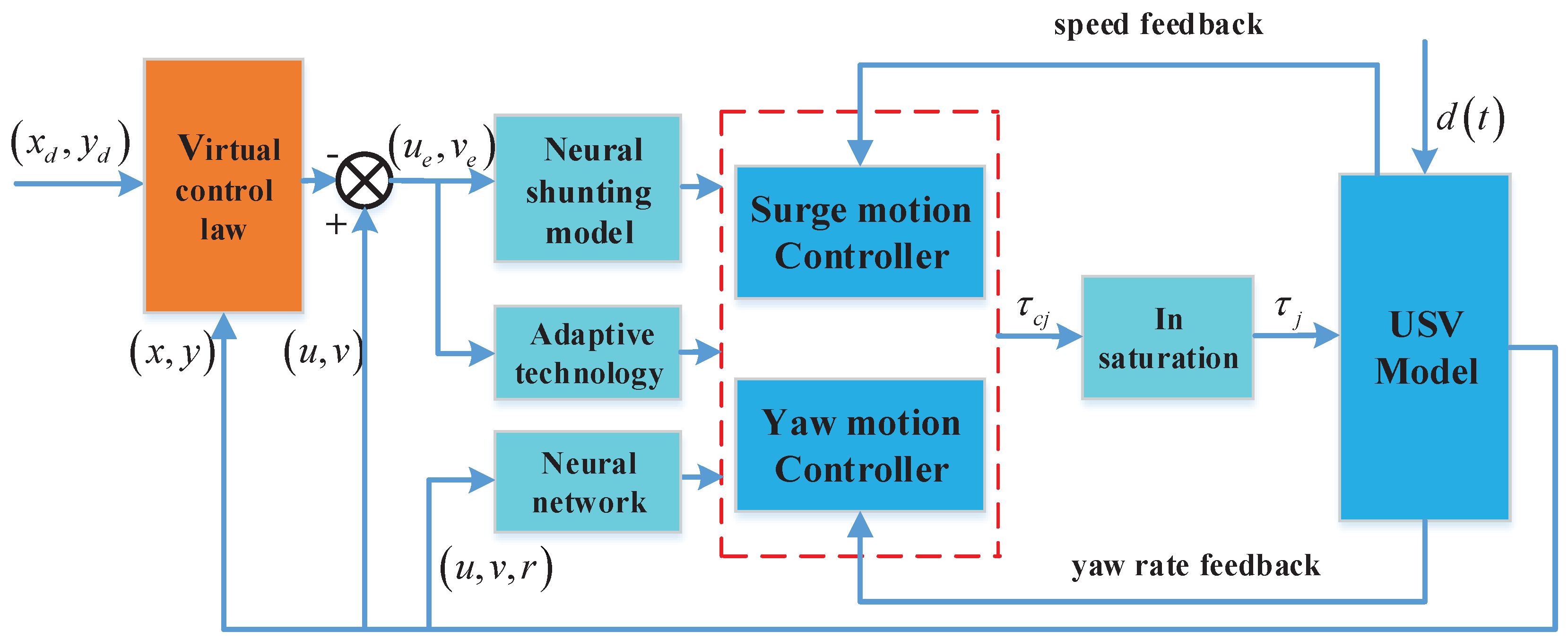
3.1. Structure of the Proposed Adaptive Control Scheme

In this subsection, a novel adaptive sliding mode trajectory tracking control strategy is proposed for the underactuated USV with unmodeled dynamics and unknown time-varying ocean disturbances. In Figure 2, the virtual control laws are designed to stabilize the position errors, and a neural shunting model is introduced to handle the “explosion of complexity” caused by the differential of the velocity tracking errors. Meanwhile, in order to enhance the stability of the system, the neural network is used to approximate unmodeled dynamics, and the adaptive technology is used to estimate the bounds of unknown time-varying disturbances. In addition, the input saturation issue is solved by hiring an auxiliary design system.

3.2. Adaptive Sliding Mode Trajectory Tracking Control Design

3.2.1. Virtual Control Law

Define the position errors

$$\begin{array}{c}\hfill \left\{\begin{array}{c}{x}_e=x-x_d\hfill \\ y_e=y-y_d\hfill \end{array}\right.\end{array}$$

(6)

Differentiating the position errors (6), we have

$$\begin{array}{c}\hfill \left\{\begin{array}{c}{\dot{x}}_e=ucos\psi -vsin\psi -{\dot{x}}_d\hfill \\ {\dot{y}}_e=usin\psi +vcos\psi -{\dot{y}}_d\hfill \end{array}\right.\end{array}$$

(7)

Define the velocity errors as

$$\begin{array}{c}\hfill \left\{\begin{array}{c}{u}_e=u-{\alpha }_u\hfill \\ v_e=v-{\alpha }_v\hfill \end{array}\right.\end{array}$$

(8)

where ${\alpha }_u$ and ${\alpha }_v$ represent virtual control laws.

In order to stabilize the position errors, the virtual control laws are designed as

$$\begin{array}{c}\hfill \left\{\begin{array}{c}{\alpha }_u={\dot{x}}_{d}cos\psi +{\dot{y}}_{d}sin\psi -\frac{\lambda x_e}{\sqrt{x_e^2+y_e^2+M}}cos\psi -\frac{\lambda y_e}{\sqrt{x_e^2+y_e^2+M}}sin\psi \hfill \\ {\alpha }_v=-{\dot{x}}_{d}sin\psi +{\dot{y}}_{d}cos\psi +\frac{\lambda x_e}{\sqrt{x_e^2+y_e^2+M}}sin\psi -\frac{\lambda y_e}{\sqrt{x_e^2+y_e^2+M}}cos\psi \hfill \end{array}\right.\end{array}$$

(9)

where $\lambda$ and M are positive constants.

Substituting (9) into (7), we obtain

$$\begin{array}{c}\hfill \left\{\begin{array}{c}{\dot{x}}_e=u_{e}cos\psi -v_{e}sin\psi -\frac{\lambda x_e}{\sqrt{x_e^2+y_e^2+M}}\hfill \\ {\dot{y}}_e=u_{e}sin\psi +v_{e}cos\psi -\frac{\lambda y_e}{\sqrt{x_e^2+y_e^2+M}}\hfill \end{array}\right.\end{array}$$

(10)

Therefore, when $u_e$ and $v_e$ converge to zero, define the Lyapunov function $V_1=\frac{1}{2}{x}_e^2+\frac{1}{2}{y}_e^2$, the time derivative of $V_1$ is written as

$$\begin{array}{cc}\hfill {\dot{V}}_1& =x_e{\dot{x}}_e+y_e{\dot{y}}_e\hfill \\ & =-\frac{\lambda \left(x_e^2+y_e^2\right)}{\sqrt{x_e^2+y_e^2+M}}\le 0\hfill \end{array}$$

(11)

According to the above analysis, as long as we can stabilize the velocity errors $u_e$ and $v_e$, the position errors $x_e$ and $y_e$ asymptotically converge to zero.

Remark 1.

In [11], when $\left|x_e\right|$ and $\left|y_e\right|$ are relatively large, the virtual control laws can exceed the velocity range of USV, and they can lead to system instability or controller crash. However, the designed virtual control laws of this paper can avoid the above problem.

3.2.2. Surge Motion Control Law

In this section, the main purpose is that the surge control law is designed to stabilize $u_e$. Meanwhile, the neural network MLP, the adaptive technology and the auxiliary dynamic system are used to handle unmodeled dynamics, unknown disturbance bounds and input saturation, respectively.

Define the velocity error sliding surface $s_1$ as

$$\begin{array}{c}\hfill s_1=u_e+{\gamma }_1{\int }_0^t{u}_e\left(\iota \right)d\iota \end{array}$$

(12)

where ${\gamma }_1$ is a positive constant.

To avoid the differential expansion, a neural shunting model is introduced to realize the differential of ${\alpha }_u$, which is expressed as

$$\begin{array}{c}\hfill {\dot{\beta }}_u=-A_u{\beta }_u+\left(B_u-{\beta }_u\right)f\left({\alpha }_u\right)-\left(D_u+{\beta }_u\right)g\left({\alpha }_u\right)\end{array}$$

(13)

where ${\dot{\beta }}_u$ denotes the output of the neural shunting model.

Remark 2.

Neural shunting model [40] originally belonged to the biological category, which has been applied to the field of robot control [41,42], and it can be expressed in the following form

$$\begin{array}{c}\hfill {\dot{\beta }}_j=-A_j{\beta }_j+\left(B_j-{\beta }_j\right)f\left({\alpha }_j\right)-\left(D_j+{\beta }_j\right)g\left({\alpha }_j\right)\end{array}$$

(14)

where $A_j$, $B_j$ and $D_j$ $\left(j=u,r\right)$ denote three design parameters, ${\alpha }_j$ and ${\beta }_j$ represent the input and output of the system, respectively. In addition, $f\left({\alpha }_j\right)$ and $g\left({\alpha }_j\right)$ represent the threshold functions of model, in which $f\left({\alpha }_j\right)=\left\{\begin{array}{c}{\alpha }_j,{\alpha }_j\ge 0\hfill \\ 0,{\alpha }_j<0\hfill \end{array}\right.$, $g\left({\alpha }_j\right)=\left\{\begin{array}{c}0,{\alpha }_j>0\hfill \\ -{\alpha }_j,{\alpha }_j\le 0\hfill \end{array}\right.$.

The derivative of $s_1$ is written as

$$\begin{array}{c}\hfill {\dot{s}}_1=\frac{1}{m_{11}}\left(m_{11}{f}_u+\Delta f_u+{\tau }_u+d_u\right)-{\dot{\beta }}_u+{\gamma }_1\left(u-{\alpha }_u\right)\end{array}$$

(15)

To reduce the chattering problem and the influence of disturbances, a sliding mode control law with hyperbolic tangent function is adopted to make the sliding surface converge to zero, which can be written as

$$\begin{array}{c}\hfill {\dot{s}}_1=-{\widehat{d}}_u^{*}tanh\left(s_1/\phantom{s_1{\epsilon }_1}{\epsilon }_1\right)-{\rho }_1{s}_1\end{array}$$

(16)

where ${\rho }_1$ and ${\epsilon }_1$ represent two design parameters, ${\widehat{d}}_u^{*}$ is the estimate of $d_u^{*}$ bound. In addition, the corresponding estimated error is ${\tilde{d}}_u^{*}=d_u^{*}-{\widehat{d}}_u^{*}$, and the adaptive law with “$\kappa$-correction” is proposed as

$$\begin{array}{c}\hfill \dot{\widehat{d_u^{*}}}={\mathsf{\Gamma }}_1\left(s_{1}tanh\left(s_1/\phantom{s_1{\epsilon }_2}{\epsilon }_1\right)-{\kappa }_1\left({\widehat{d}}_u^{*}-d_{u0}^{*}\right)\right)\end{array}$$

(17)

where ${\mathsf{\Gamma }}_1$ and ${\kappa }_1$ are positive design parameters, $d_{u0}^{*}$ is the initial value.

Then the surge motion control law is designed as

$$\begin{array}{c}\hfill {\tau }_{cu}=-m_{11}{f}_u-\Delta {\widehat{f}}_u+m_{11}{\dot{\beta }}_u-{\gamma }_1{m}_{11}{u}_e-{\widehat{d}}_u^{*}tanh\left(s_1/\phantom{s_1{\epsilon }_2}{\epsilon }_1\right)-{\rho }_1{s}_1\end{array}$$

(18)

where $\Delta {\widehat{f}}_u=\frac{1}{2}{s}_1{\widehat{\vartheta }}_1{\mathsf{\Theta }}^T\mathsf{\Theta }$ is the estimate of $f_u$, the corresponding adaptive law is

$$\begin{array}{c}\hfill {\dot{\widehat{\vartheta }}}_1={\varsigma }_1\left(\frac{1}{2}{s}_1^2{\mathsf{\Theta }}^T\mathsf{\Theta }-{\varphi }_1{\widehat{\vartheta }}_1\right)\end{array}$$

(19)

where ${\varsigma }_1$ and ${\varphi }_1$ are positive constants. In addition, the estimated error is ${\tilde{\vartheta }}_1={\vartheta }_1-{\widehat{\vartheta }}_1$.

In order to deal with the problem of input saturation (2), an auxiliary dynamic system [43,44] is constructed as

$$\begin{array}{c}\hfill {\dot{\zeta }}_u=\left\{\begin{array}{cc}-K_{\zeta u}{\zeta }_u-\frac{\left|s_1\Delta {\tau }_u\right|+0.5\Delta {\tau }_u^2}{∥{\zeta }_u^2∥}·{\zeta }_u+\Delta {\tau }_u,\hfill & ∥{\zeta }_u∥\ge {\sigma }_u\hfill \\ 0,\hfill & ∥{\zeta }_u∥<{\sigma }_u\hfill \end{array}\right.\end{array}$$

(20)

where ${\zeta }_u$ is a state variable, $\Delta {\tau }_u={\tau }_u-{\tau }_{cu}$, $K_{\zeta u}$ is a positive constant, and ${\sigma }_u>0$ is a small design constant.

The surge motion control law ${\tau }_{cu}$ can be modified by

$$\begin{array}{c}\hfill {\tau }_{cu}=-\frac{1}{2}{s}_1{\widehat{\vartheta }}_1{\mathsf{\Theta }}^T\mathsf{\Theta }+h_1-{\widehat{d}}_u^{*}tanh\left(s_1/{\epsilon }_1\right)-{\rho }_1{s}_1+k_{s1}{\zeta }_u\end{array}$$

(21)

where $h_1=m_{11}{\dot{\beta }}_u-{\gamma }_1{m}_{11}{u}_e-m_{11}{f}_u$, $k_{s1}$ is a positive design parameter.

3.2.3. Yaw Motion Control Law

A second-order sliding surface is defined as

$$\begin{array}{c}\hfill s_2={\dot{v}}_e+{\gamma }_2{v}_e\end{array}$$

(22)

where ${\gamma }_2$ is a positive constant.

The time derivative of (22) is

$$\begin{array}{c}\hfill {\dot{s}}_2=\ddot{v}-{\ddot{\alpha }}_v+{\gamma }_2\left(\dot{v}-{\dot{\alpha }}_v\right)\end{array}$$

(23)

where ${\dot{\alpha }}_v=\chi -r{\alpha }_u$, in which

$$\begin{array}{c}\chi =-\left({\ddot{x}}_d-\lambda \left({\mu }^{-1}-{\mu }^{-3}{x}_e^2\right){\dot{x}}_e+\lambda {\mu }^{-3}{x}_e{y}_e{\dot{y}}_e\right)sin\psi \hfill \\ +\left({\ddot{y}}_d-\lambda \left({\mu }^{-1}-{\mu }^{-3}{y}_e^2\right){\dot{y}}_e+\lambda {\mu }^{-3}{x}_e{y}_e{\dot{x}}_e\right)cos\psi \hfill \end{array}$$

(24)

where $\mu =\sqrt{x_e^2+y_e^2+M}$.

From Remark 2, to further avoid the computational explosion in the time derivative of $\chi$, let $\chi$ pass a neural shunting model, which can be written as

$$\begin{array}{c}\hfill {\dot{\beta }}_r=-A_r{\beta }_r+\left(B_r-{\beta }_r\right)f\left(\chi \right)-\left(D_r+{\beta }_r\right)g\left(\chi \right)\end{array}$$

(25)

where ${\dot{\beta }}_r$ denotes the output of the neural shunting model.

Then the time derivative of ${\dot{\alpha }}_v$ is

$$\begin{array}{c}\hfill {\ddot{\alpha }}_v={\dot{\beta }}_r-\dot{r}{\alpha }_u-r{\dot{\alpha }}_u\end{array}$$

(26)

Combining (4), (13), (25) and (26), we have

$$\begin{array}{c}\hfill {\dot{s}}_2=r{\dot{\beta }}_u-{\dot{\beta }}_r+{\gamma }_2\left(\dot{v}-{\dot{\alpha }}_v\right)+\frac{{\alpha }_u}{m_{33}}\left(m_{33}{f}_r+{\tau }_{cr}+d_r\right)+\frac{\Delta f_m}{m_{33}}\end{array}$$

(27)

where $\Delta f_m=m_{33}\ddot{v}+{\alpha }_u\Delta f_r$.

Similarly, a hyperbolic tangent function is used to reduce the chattering problem, and we have

$$\begin{array}{c}\hfill {\dot{s}}_2=-{\widehat{d}}_r^{*}tanh\left(s_2/\phantom{s_2{\epsilon }_2}{\epsilon }_2\right)-{\rho }_2{s}_2\end{array}$$

(28)

where ${\rho }_2$ and ${\epsilon }_2$ are two design parameters, ${\widehat{d}}_r^{*}$ is the estimate of $d_r^{*}$, and the estimated error is ${\tilde{d}}_r^{*}=d_r^{*}-{\widehat{d}}_r^{*}$. The adaptive law with “$\kappa$-correction” is selected as

$$\begin{array}{c}\hfill \dot{\widehat{d_r^{*}}}={\mathsf{\Gamma }}_2\left(s_{2}tanh\left(s_2/{\epsilon }_2\right)-{\kappa }_2\left({\widehat{d}}_r^{*}-d_{r0}^{*}\right)\right)\end{array}$$

(29)

where ${\mathsf{\Gamma }}_2$ and ${\kappa }_2$ represent positive constants, $d_{r0}^{*}$ is the initial value.

Then the yaw motion control law is designed as

$$\begin{array}{c}\hfill {\tau }_{cr}=\frac{1}{{\alpha }_u}\left(m_{33}\left({\dot{\beta }}_r-r{\dot{\beta }}_u-{\gamma }_2\left(\dot{v}-{\dot{\alpha }}_v\right)\right)-\Delta {\widehat{f}}_m-{\widehat{d}}_r^{*}tanh\left(s_2/{\epsilon }_2\right)-{\rho }_2{s}_2\right)-m_{33}{f}_r\end{array}$$

(30)

where $\Delta {\widehat{f}}_m=\frac{1}{2}{s}_2{\widehat{\vartheta }}_2{\mathsf{\Theta }}^T\mathsf{\Theta }$, the corresponding adaptive law is

$$\begin{array}{c}\hfill {\dot{\widehat{\vartheta }}}_2={\varsigma }_2\left(\frac{1}{2}{s}_2^2{\mathsf{\Theta }}^T\mathsf{\Theta }-{\varphi }_2{\widehat{\vartheta }}_2\right)\end{array}$$

(31)

where ${\varsigma }_2$ and ${\varphi }_2$ are positive constants, and the estimated error is ${\tilde{\vartheta }}_2={\vartheta }_2-{\widehat{\vartheta }}_2$.

For the input saturation problem of the yaw motion control, the auxiliary dynamic system is designed as

$$\begin{array}{c}\hfill {\dot{\zeta }}_r=\left\{\begin{array}{cc}-K_{\zeta r}{\zeta }_r-\frac{\left|s_2\Delta {\tau }_r\right|+0.5\Delta {\tau }_r^2}{∥{\zeta }_r^2∥}·{\zeta }_r+\Delta {\tau }_r,\hfill & ∥{\zeta }_r∥\ge {\sigma }_r\hfill \\ 0,\hfill & ∥{\zeta }_r∥<{\sigma }_r\hfill \end{array}\right.\end{array}$$

(32)

where ${\zeta }_r$ is a state variable, $\Delta {\tau }_r={\tau }_r-{\tau }_{cr}$, $K_{\zeta r}$ is a positive constant, and ${\sigma }_r>0$ is a small design constant.

The yaw motion control law ${\tau }_{cr}$ is modified by

$$\begin{array}{c}\hfill {\tau }_{cr}=\frac{1}{{\alpha }_u}\left(h_2-\frac{1}{2}{s}_2{\widehat{\vartheta }}_2{\mathsf{\Theta }}^T\mathsf{\Theta }-{\widehat{d}}_r^{*}tanh\left(s_2/{\epsilon }_2\right)-{\rho }_2{s}_2+k_{s2}{\zeta }_r\right)-m_{33}{f}_r\end{array}$$

(33)

where $h_2=m_{33}\left({\dot{\beta }}_r-r{\dot{\beta }}_u-{\gamma }_2\left(\dot{v}-{\dot{\alpha }}_v\right)\right)$, $k_{s2}$ is a positive design parameter.

Remark 3.

In practice, the surge velocity satisfies $u⩾0$. From (30), ${\tau }_r$ will produce singular value when ${\alpha }_u=0$. Through the assumption $m_{22}{\alpha }_u-m_{11}u>0$ in [28], we have ${\alpha }_u\ne 0$.

4. Stability Analysis

Define the errors ${\mathsf{\Phi }}_u$ and ${\mathsf{\Phi }}_r$

$$\begin{array}{c}\hfill \left\{\begin{array}{c}{\mathsf{\Phi }}_u={\beta }_u-{\alpha }_u\hfill \\ {\mathsf{\Phi }}_r={\beta }_r-\chi \hfill \end{array}\right.\end{array}$$

(34)

The time derivative of ${\mathsf{\Phi }}_u$ is

$$\begin{array}{cc}\hfill {\dot{\mathsf{\Phi }}}_u& ={\dot{\beta }}_u-{\dot{\alpha }}_u\hfill \\ & =-\left(A_u+f\left({\alpha }_u\right)+g\left({\alpha }_u\right)\right){\beta }_u+\left(B_{u}f\left({\alpha }_u\right)-D_{u}g\left({\alpha }_u\right)\right)-X_u\hfill \end{array}$$

(35)

where $X_u=\frac{\partial {\alpha }_u}{\partial {\dot{x}}_d}{\ddot{x}}_d+\frac{\partial {\alpha }_u}{\partial {\ddot{y}}_d}{\ddot{y}}_d+\frac{\partial {\alpha }_u}{\partial x_e}{\dot{x}}_e+\frac{\partial {\alpha }_u}{\partial y_e}{\dot{y}}_e+\frac{\partial {\alpha }_u}{\partial \psi }\dot{\psi }$.

According to the nature of the neural shunting model, if $B_u=D_u$, we have

$$\begin{array}{c}\hfill {\dot{\mathsf{\Phi }}}_u=-{\theta }_u{\beta }_u+B_u{\alpha }_u-X_u\end{array}$$

(36)

where ${\theta }_u=A_u+f\left({\alpha }_u\right)+g\left({\alpha }_u\right)$.

Similarly, if $B_r=D_r$, the time derivative of ${\mathsf{\Phi }}_r$ is

$$\begin{array}{c}\hfill {\dot{\mathsf{\Phi }}}_r=-{\theta }_r{\beta }_r+B_r\chi -X_r\end{array}$$

(37)

where ${\theta }_r=A_r+f\left(\chi \right)+g\left(\chi \right)$, $X_r=\frac{\partial \chi }{\partial {\ddot{x}}_d}{\stackrel{⃛}{x}}_d+\frac{\partial \chi }{\partial {\ddot{y}}_d}{\stackrel{⃛}{y}}_d+\frac{\partial \chi }{\partial {\dot{x}}_e}{\ddot{x}}_e+\frac{\partial \chi }{\partial {\dot{y}}_e}{\ddot{y}}_e+\frac{\partial \chi }{\partial \psi }\dot{\psi }$.

Remark 4.

[10] $X_u$ and $X_r$ are bounded by $\left|X_u\right|\le {\overline{X}}_u$ and $\left|X_r\right|\le {\overline{X}}_r$, where ${\overline{X}}_u$ and ${\overline{X}}_r$ are normal numbers.

Lemma 1.

[45] For any $\epsilon >0$ and $\xi \in R$, the following inequality can be satisfied

$$\begin{array}{c}\hfill 0\le \left|\xi \right|-\xi tanh\left(\xi /\phantom{\xi \epsilon }\epsilon \right)\le {\kappa }_3\epsilon \end{array}$$

(38)

where ${\kappa }_3$ is a constant that satisfies ${\kappa }_3=e^{-\left({\kappa }_3+1\right)}$.

Theorem 1.

Consider the underactuated USV model (3) and (4) in the presence of unmodeled dynamics and unknown disturbances, suppose that Assumption 1 and Assumption 2 are satisfied, under the surge control law (21) and the yaw motion law (33), together with the adaptive laws (17), (19), (29) and (31), from the appropriately chosen parameters λ, M, ${\gamma }_1$, ${\gamma }_2$, ${\rho }_1$, ${\rho }_2$, ${\epsilon }_1$, ${\epsilon }_2$, ${\mathsf{\Gamma }}_1$, ${\mathsf{\Gamma }}_2$, ${\kappa }_1$, ${\kappa }_2$, ${\zeta }_1$, ${\zeta }_2$, ${\varsigma }_1$, ${\varphi }_2$, $K_{\zeta u}$, $K_{\zeta r}$, $k_{s1}$ and $k_{s2}$, all signals in the closed-loop system are guaranteed to be semi-globally uniformly ultimately bounded (UUB).

Proof of Theorem 1. 

Consider the following Lyapunov function

$$\begin{array}{c}\hfill V=\frac{1}{2}{m}_{11}{s}_1^2+\frac{1}{2}{m}_{33}{s}_2^2+\frac{1}{2}{\mathsf{\Gamma }}_1^{-1}\tilde{d}{{}_u^{*}}^2+\frac{1}{2}{\mathsf{\Gamma }}_2^{-1}\tilde{d}{{}_v^{*}}^2+\frac{1}{2}{\varsigma }_1^{-1}{\tilde{\vartheta }}_1^2+\frac{1}{2}{\varsigma }_2^{-1}{\tilde{\vartheta }}_2^2+\frac{1}{2}\sum _{i=u,r}\left({\mathsf{\Phi }}_i^2+{\zeta }_i^2\right)\end{array}$$

(39)

The time derivative of (39) is

$$\begin{array}{c}\hfill \dot{V}=m_{11}{s}_1{\dot{s}}_1+m_{33}{s}_2{\dot{s}}_2+{\mathsf{\Gamma }}_1^{-1}{\tilde{d}}_u^{*}\dot{\widetilde{d_u^{*}}}+{\mathsf{\Gamma }}_2^{-1}{\tilde{d}}_v^{*}\dot{\widetilde{d_v^{*}}}+{\varsigma }_1^{-1}{\tilde{\vartheta }}_1{\dot{\tilde{\vartheta }}}_1+{\varsigma }_2^{-1}{\tilde{\vartheta }}_2{\dot{\tilde{\vartheta }}}_2+\sum _{i=u,r}\left({\mathsf{\Phi }}_i{\dot{\mathsf{\Phi }}}_i+{\zeta }_i{\dot{\zeta }}_i\right)\end{array}$$

(40)

Substituting (15), (17), (27), (29) into (40) yields

$$\begin{array}{cc}\hfill \dot{V}& =s_1\left(W_u^T\mathsf{\Theta }+{\epsilon }_u-\frac{1}{2}{s}_1{\widehat{\vartheta }}_1{\mathsf{\Theta }}^T\mathsf{\Theta }-{\rho }_1{s}_1+d_u^{*}-{\widehat{d}}_u^{*}tanh\left(s_1/\phantom{s_1{\epsilon }_1}{\epsilon }_1\right)+k_{s1}{\zeta }_u+\Delta {\tau }_u\right)\hfill \\ \hfill & +s_2\left(W_m^T\mathsf{\Theta }+{\epsilon }_m-\frac{1}{2}{s}_2{\widehat{\vartheta }}_2{\mathsf{\Theta }}^T\mathsf{\Theta }-{\rho }_2{s}_2+d_r^{*}-{\widehat{d}}_r^{*}tanh\left(s_2/\phantom{s_2{\epsilon }_2}{\epsilon }_2\right)+k_{s2}{\zeta }_r+\Delta {\tau }_r\right)\hfill \\ \hfill & -{\tilde{d}}_u^{*}\left(tanh\left(s_1/\phantom{s_1{\epsilon }_1}{\epsilon }_1\right)-{\kappa }_1\left({\widehat{d}}_u^{*}-d_{u0}^{*}\right)\right)-{\tilde{d}}_r^{*}\left(tanh\left(s_2/\phantom{s_2{\epsilon }_2}{\epsilon }_2\right)-{\kappa }_2\left({\widehat{d}}_r^{*}-d_{r0}^{*}\right)\right)\hfill \\ \hfill & +{\varsigma }_1^{-1}{\tilde{\vartheta }}_1{\dot{\tilde{\vartheta }}}_1+{\varsigma }_2^{-1}{\tilde{\vartheta }}_2{\dot{\tilde{\vartheta }}}_2+\sum _{i=u,r}\left({\mathsf{\Phi }}_i{\dot{\mathsf{\Phi }}}_i+{\zeta }_i{\dot{\zeta }}_i\right)\hfill \\ \hfill & \le s_1{W}_u^T\mathsf{\Theta }+{\epsilon }_u{s}_1-\frac{1}{2}{s}_1^2{\widehat{\vartheta }}_1{\mathsf{\Theta }}^T\mathsf{\Theta }-{\rho }_1{s}_1^2+d_u^{*}\left(\left|s_1\right|-s_{1}tanh\left(s_1/\phantom{s_1{\epsilon }_1}{\epsilon }_1\right)\right)+k_{s1}{s}_1{\zeta }_u\hfill \\ \hfill & +s_2{W}_m^T\mathsf{\Theta }+{\epsilon }_m{s}_2-\frac{1}{2}{s}_2^2{\widehat{\vartheta }}_2{\mathsf{\Theta }}^T\mathsf{\Theta }-{\rho }_2{s}_2^2+d_r^{*}\left(\left|s_2\right|-s_{2}tanh\left(s_2/\phantom{s_2{\epsilon }_2}{\epsilon }_2\right)\right)+k_{s2}{s}_2{\zeta }_r\hfill \\ \hfill & +{\kappa }_1\left(d_u^{*}-{\widehat{d}}_u^{*}\right)\left({\widehat{d}}_u^{*}-d_{u0}^{*}\right)+{\kappa }_2\left(d_r^{*}-{\widehat{d}}_r^{*}\right)\left({\widehat{d}}_r^{*}-d_{r0}^{*}\right)+{\varsigma }_1^{-1}{\tilde{\vartheta }}_1{\dot{\tilde{\vartheta }}}_1+{\varsigma }_2^{-1}{\tilde{\vartheta }}_2{\dot{\tilde{\vartheta }}}_2\hfill \\ \hfill & +\Delta {\tau }_u{s}_1+\Delta {\tau }_r{s}_2+\sum _{i=u,r}\left({\mathsf{\Phi }}_i{\dot{\mathsf{\Phi }}}_i+{\zeta }_i{\dot{\zeta }}_i\right)\hfill \end{array}$$

(41)

According to Young’s inequality, we have

$$\begin{array}{c}\hfill \begin{array}{c}2s_1{W}_u^T\mathsf{\Theta }\le s_1^2{\vartheta }_1{\mathsf{\Theta }}^T\mathsf{\Theta }+1\hfill \\ 2s_2{W}_m^T\mathsf{\Theta }\le s_2^2{\vartheta }_2{\mathsf{\Theta }}^T\mathsf{\Theta }+1\hfill \end{array}\end{array}$$

(42)

$$\begin{array}{c}\hfill \begin{array}{c}{\kappa }_1\left(d_u^{*}-{\widehat{d}}_u^{*}\right)\left({\widehat{d}}_u^{*}-d_{u0}^{*}\right)\le -\frac{{\kappa }_1}{2}{\left(d_u^{*}-{\widehat{d}}_u^{*}\right)}^2+\frac{{\kappa }_1}{2}{\left(d_u^{*}-d_{u0}^{*}\right)}^2\hfill \\ {\kappa }_2\left(d_r^{*}-{\widehat{d}}_r^{*}\right)\left({\widehat{d}}_r^{*}-d_{r0}^{*}\right)\le -\frac{{\kappa }_2}{2}{\left(d_r^{*}-{\widehat{d}}_r^{*}\right)}^2+\frac{{\kappa }_2}{2}{\left(d_r^{*}-d_{r0}^{*}\right)}^2\hfill \end{array}\end{array}$$

(43)

From Lemma 1, (42) and (43), we obtain

$$\begin{array}{cc}\hfill \dot{V}& \le {\epsilon }_u{s}_1-{\rho }_1{s}_1^2+\frac{1}{2}{s}_1^2{\tilde{\vartheta }}_1{\mathsf{\Theta }}^T\mathsf{\Theta }+d_u^{*}{\kappa }_3{\epsilon }_1+k_{s1}{s}_1{\zeta }_u+{\epsilon }_m{s}_2-{\rho }_2{s}_2^2+\frac{1}{2}{s}_2^2{\tilde{\vartheta }}_2{\mathsf{\Theta }}^T\mathsf{\Theta }\hfill \\ \hfill & +d_r^{*}{\kappa }_3{\epsilon }_2+k_{s2}{s}_2{\zeta }_r-\frac{{\kappa }_1}{2}{\left(d_u^{*}-{\widehat{d}}_u^{*}\right)}^2+\frac{{\kappa }_1}{2}{\left(d_u^{*}-d_{u0}^{*}\right)}^2-\frac{{\kappa }_2}{2}{\left(d_r^{*}-{\widehat{d}}_r^{*}\right)}^2+\frac{{\kappa }_2}{2}{\left(d_r^{*}-d_{r0}^{*}\right)}^2\hfill \\ \hfill & -{\tilde{\vartheta }}_1\left(\frac{1}{2}{s}_1^2{\mathsf{\Theta }}^T\mathsf{\Theta }-{\varphi }_1{\widehat{\vartheta }}_1\right)-{\tilde{\vartheta }}_2\left(\frac{1}{2}{s}_2^2{\mathsf{\Theta }}^T\mathsf{\Theta }-{\varphi }_2{\widehat{\vartheta }}_2\right)+\Delta {\tau }_u{s}_1+\Delta {\tau }_r{s}_2+\sum _{i=u,r}\left({\mathsf{\Phi }}_i{\dot{\mathsf{\Phi }}}_i+{\zeta }_i{\dot{\zeta }}_i\right)+1\hfill \\ \hfill & \le {\epsilon }_u{s}_1-{\rho }_1{s}_1^2+d_u^{*}{\kappa }_3{\epsilon }_1+k_{s1}{s}_1{\zeta }_u+{\epsilon }_m{s}_2-{\rho }_2{s}_2^2+d_r^{*}{\kappa }_3{\epsilon }_2+k_{s2}{s}_2{\zeta }_r-\frac{{\kappa }_1}{2}{\left(d_u^{*}-{\widehat{d}}_u^{*}\right)}^2\hfill \\ \hfill & +\frac{{\kappa }_1}{2}{\left(d_u^{*}-d_{u0}^{*}\right)}^2-\frac{{\kappa }_2}{2}{\left(d_r^{*}-{\widehat{d}}_r^{*}\right)}^2+\frac{{\kappa }_2}{2}{\left(d_r^{*}-d_{r0}^{*}\right)}^2+{\varphi }_1{\tilde{\vartheta }}_1{\widehat{\vartheta }}_1+{\varphi }_2{\tilde{\vartheta }}_2{\widehat{\vartheta }}_2\hfill \\ \hfill & +\Delta {\tau }_u{s}_1+\Delta {\tau }_r{s}_2+\sum _{i=u,r}\left({\mathsf{\Phi }}_i{\dot{\mathsf{\Phi }}}_i+{\zeta }_i{\dot{\zeta }}_i\right)+1\hfill \end{array}$$

(44)

Define ${\theta }_i=B_i$, substituting (34), (36) and (37) into (44) yields

$$\begin{array}{cc}\hfill \dot{V}& \le {\epsilon }_u{s}_1-{\rho }_1{s}_1^2+{\epsilon }_m{s}_2-{\rho }_2{s}_2^2+d_u^{*}{\kappa }_3{\epsilon }_1+d_r^{*}{\kappa }_3{\epsilon }_2+k_{s1}{s}_1{\zeta }_u+k_{s2}{s}_2{\zeta }_r\hfill \\ \hfill & -\frac{{\kappa }_1}{2}{\left(d_u^{*}-{\widehat{d}}_u^{*}\right)}^2-\frac{{\kappa }_2}{2}{\left(d_r^{*}-{\widehat{d}}_r^{*}\right)}^2-{\theta }_u{\mathsf{\Theta }}_u^2-{\theta }_v{\mathsf{\Theta }}_v^2+\frac{{\kappa }_1}{2}{\left(d_u^{*}-d_{u0}^{*}\right)}^2\hfill \\ \hfill & +\frac{{\kappa }_2}{2}{\left(d_r^{*}-d_{r0}^{*}\right)}^2+{\varphi }_1{\tilde{\vartheta }}_1{\widehat{\vartheta }}_1+{\varphi }_2{\tilde{\vartheta }}_2{\widehat{\vartheta }}_2+\Delta {\tau }_u{s}_1+\Delta {\tau }_r{s}_2-{\mathsf{\Phi }}_u{X}_u-{\mathsf{\Phi }}_v{X}_v\hfill \\ \hfill & +\sum _{i=u,r}\left({\zeta }_i{\dot{\zeta }}_i\right)+1\hfill \end{array}$$

(45)

It is clear that ${\zeta }_u{\dot{\zeta }}_u=-K_{\zeta u}{\zeta }_u^2-\frac{\left|s_1\Delta {\tau }_u\right|+0.5\Delta {\tau }_u^2}{∥{\zeta }_u^2∥}·{\zeta }_u^2+\Delta {\tau }_u{\zeta }_u$, $2\Delta {\tau }_u{\zeta }_u\le \Delta {\tau }_u^2+{\zeta }_u^2$. Similarly, ${\zeta }_r$ also satisfies the above conditions. Thus we have

$$\begin{array}{cc}\hfill \dot{V}& \le {\epsilon }_u{s}_1-{\rho }_1{s}_1^2+{\epsilon }_m{s}_2-{\rho }_2{s}_2^2+d_u^{*}{\kappa }_3{\epsilon }_1+d_r^{*}{\kappa }_3{\epsilon }_2+k_{s1}{s}_1{\zeta }_u+k_{s2}{s}_2{\zeta }_r\hfill \\ \hfill & -\frac{{\kappa }_1}{2}{\left(d_u^{*}-{\widehat{d}}_u^{*}\right)}^2-\frac{{\kappa }_2}{2}{\left(d_r^{*}-{\widehat{d}}_r^{*}\right)}^2-{\theta }_u{\mathsf{\Theta }}_u^2-{\theta }_v{\mathsf{\Theta }}_v^2+\frac{{\kappa }_1}{2}{\left(d_u^{*}-d_{u0}^{*}\right)}^2\hfill \\ \hfill & +\frac{{\kappa }_2}{2}{\left(d_r^{*}-d_{r0}^{*}\right)}^2+{\varphi }_1{\tilde{\vartheta }}_1{\widehat{\vartheta }}_1+{\varphi }_2{\tilde{\vartheta }}_2{\widehat{\vartheta }}_2-{\mathsf{\Phi }}_u{X}_u-{\mathsf{\Phi }}_r{X}_r\hfill \\ \hfill & -\left(K_{\zeta u}-\frac{1}{2}\right){\zeta }_u^2-\left(K_{\zeta r}-\frac{1}{2}\right){\zeta }_r^2+1\hfill \end{array}$$

(46)

Through inequality $2{\tilde{\vartheta }}_1{\widehat{\vartheta }}_1\le {\vartheta }_1^2-{\tilde{\vartheta }}_1^2$, $2{\tilde{\vartheta }}_2{\widehat{\vartheta }}_2\le {\vartheta }_2^2-{\tilde{\vartheta }}_2^2$ and Young’s inequality, we obtain

$$\begin{array}{cc}\hfill \dot{V}& \le -\frac{1}{2}\left({\rho }_1-k_{s1}-1\right)s_1^2-\frac{1}{2}\left({\rho }_2-k_{s2}-1\right)s_2^2-\frac{{\kappa }_1}{2}{\left(d_u^{*}-{\widehat{d}}_u^{*}\right)}^2-\frac{{\kappa }_2}{2}{\left(d_r^{*}-{\widehat{d}}_r^{*}\right)}^2\hfill \\ \hfill & -\frac{{\varphi }_1}{2}{\tilde{\vartheta }}_1^2-\frac{{\varphi }_2}{2}{\tilde{\vartheta }}_2^2-\left({\theta }_u-\frac{1}{2}\right){\mathsf{\Theta }}_u^2-\left({\theta }_r-\frac{1}{2}\right){\mathsf{\Theta }}_r^2-\left(K_{\zeta u}-\frac{1}{2}{k}_{s1}-\frac{1}{2}\right){\zeta }_u^2\hfill \\ \hfill & -\left(K_{\zeta r}-\frac{1}{2}{k}_{s2}-\frac{1}{2}\right){\zeta }_r^2+\frac{{\kappa }_1}{2}{\left(d_u^{*}-d_{u0}^{*}\right)}^2+\frac{{\kappa }_2}{2}{\left(d_r^{*}-d_{r0}^{*}\right)}^2+\frac{{\varphi }_1}{2}{\vartheta }_1^2\hfill \\ \hfill & +\frac{{\varphi }_2}{2}{\vartheta }_2^2+\frac{1}{2}{\overline{X}}_u^2+\frac{1}{2}{\overline{X}}_r^2+\frac{1}{2}{\epsilon }_u^2+\frac{1}{2}{\epsilon }_m^2+d_u^{*}{\kappa }_3{\epsilon }_1+d_r^{*}{\kappa }_3{\epsilon }_2+1\hfill \end{array}$$

(47)

Set $S_1=\frac{1}{2}\left({\rho }_1-k_{s1}-1\right)>0$, $S_2=\frac{1}{2}\left({\rho }_2-k_{s2}-1\right)>0$, $S_3=\frac{{\kappa }_1}{2}$, $S_4=\frac{{\kappa }_2}{2}$, $S_5=\frac{{\varphi }_1}{2}$, $S_6=\frac{{\varphi }_2}{2}$, $S_7={\theta }_u-\frac{1}{2}>0$, $S_8={\theta }_v-\frac{1}{2}>0$, $S_9=\left(K_{\zeta u}-\frac{1}{2}{k}_{s1}-\frac{1}{2}\right)>0$, $S_{10}=\left(K_{\zeta r}-\frac{1}{2}{k}_{s2}-\frac{1}{2}\right)>0$, $\mathsf{\Lambda }=\frac{{\kappa }_1}{2}{\left(d_u^{*}-d_{u0}^{*}\right)}^2+\frac{{\kappa }_2}{2}{\left(d_r^{*}-d_{r0}^{*}\right)}^2+\frac{{\varphi }_1}{2}{\vartheta }_1^2+\frac{{\varphi }_2}{2}{\vartheta }_2^2+\frac{1}{2}{\overline{X}}_u^2+\frac{1}{2}{\overline{X}}_r^2+\frac{1}{2}{\epsilon }_u^2+\frac{1}{2}{\epsilon }_m^2+d_u^{*}{\kappa }_3{\epsilon }_1+d_r^{*}{\kappa }_3{\epsilon }_2+1$. Then (47) can be written as

$$\begin{array}{c}\hfill \dot{V}\le -S_1{s}_1^2-S_2{s}_2^2-S_3\tilde{d}{{}_u^{*}}^2-S_4\tilde{d}{{}_r^{*}}^2-S_5{\tilde{\vartheta }}_1^2-S_6{\tilde{\vartheta }}_2^2-S_7{\mathsf{\Theta }}_u^2-S_8{\mathsf{\Theta }}_r^2-S_9{\zeta }_u^2-S_{10}{\zeta }_r^2+\mathsf{\Lambda }\end{array}$$

(48)

Define $S:=min\left\{S_1,S_2,S_3,S_4,S_5,S_6,S_7,S_8,S_9,S_{10}\right\}$, we have

$$\begin{array}{c}\hfill \dot{V}\le -2SV+\mathsf{\Lambda }\end{array}$$

(49)

Solving (49), we obtain the following inequality

$$\begin{array}{cc}\hfill V& \le \left(V\left(0\right)-\frac{\mathsf{\Lambda }}{2S}\right)e^{-2St}+\frac{\mathsf{\Lambda }}{2S}\hfill \\ & \le V\left(0\right)e^{-2St}+\frac{\mathsf{\Lambda }}{2S},\forall t>0\hfill \end{array}$$

(50)

Based on the above analysis, it is clear from (50) that V is bounded by $\frac{\mathsf{\Lambda }}{2S}$. Thus, the formation errors are guaranteed to be uniformly ultimately bounded. □

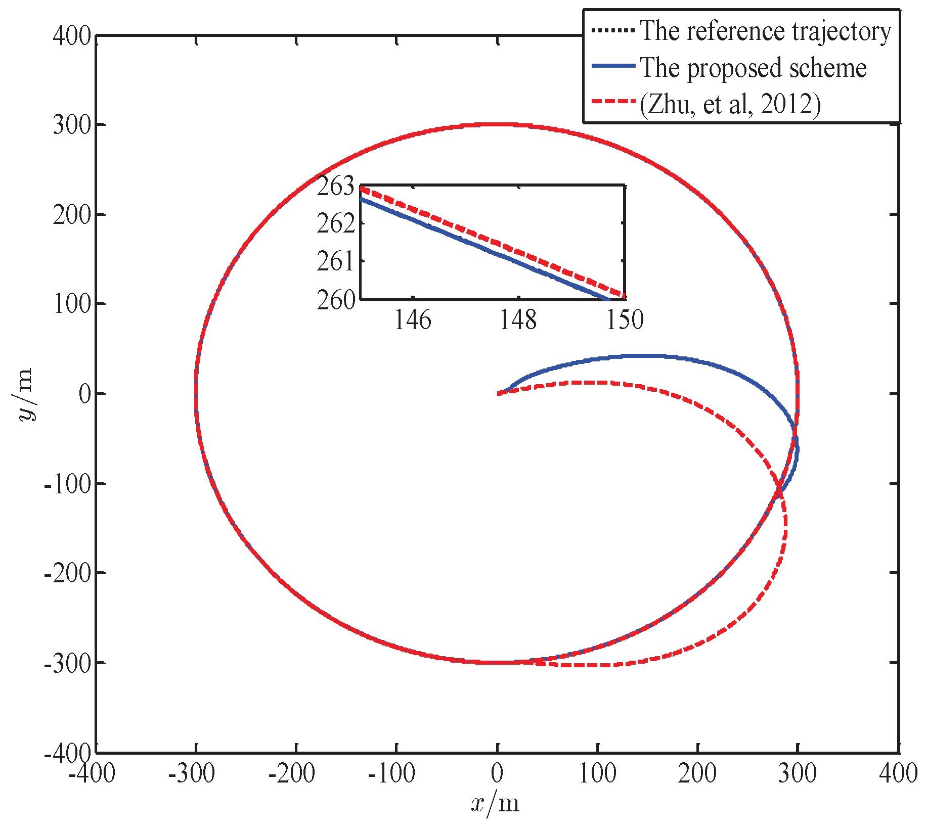
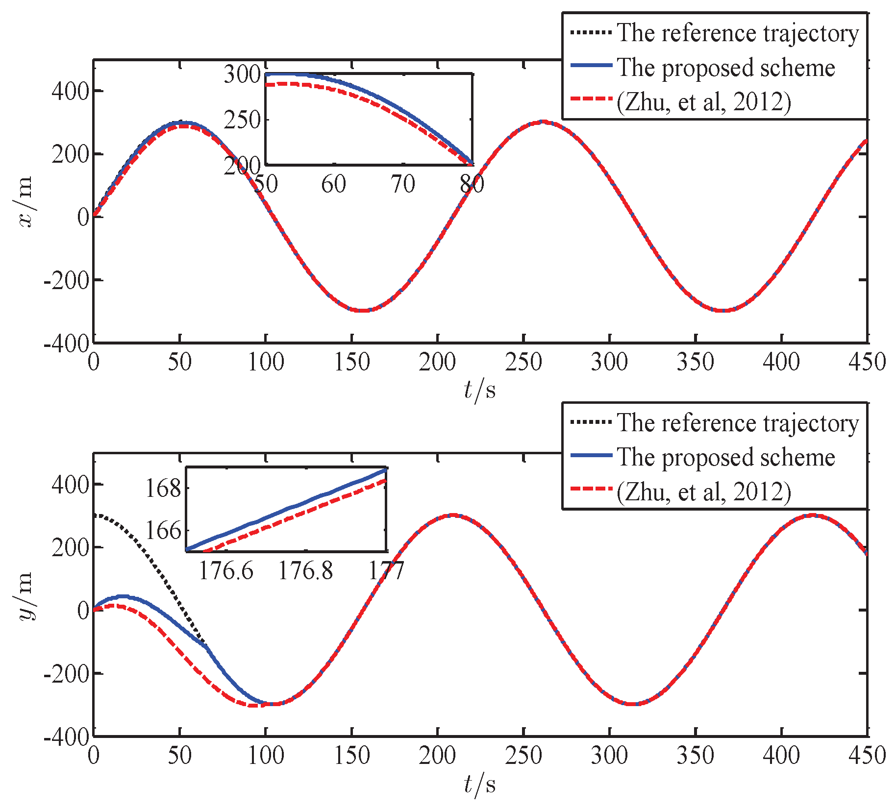
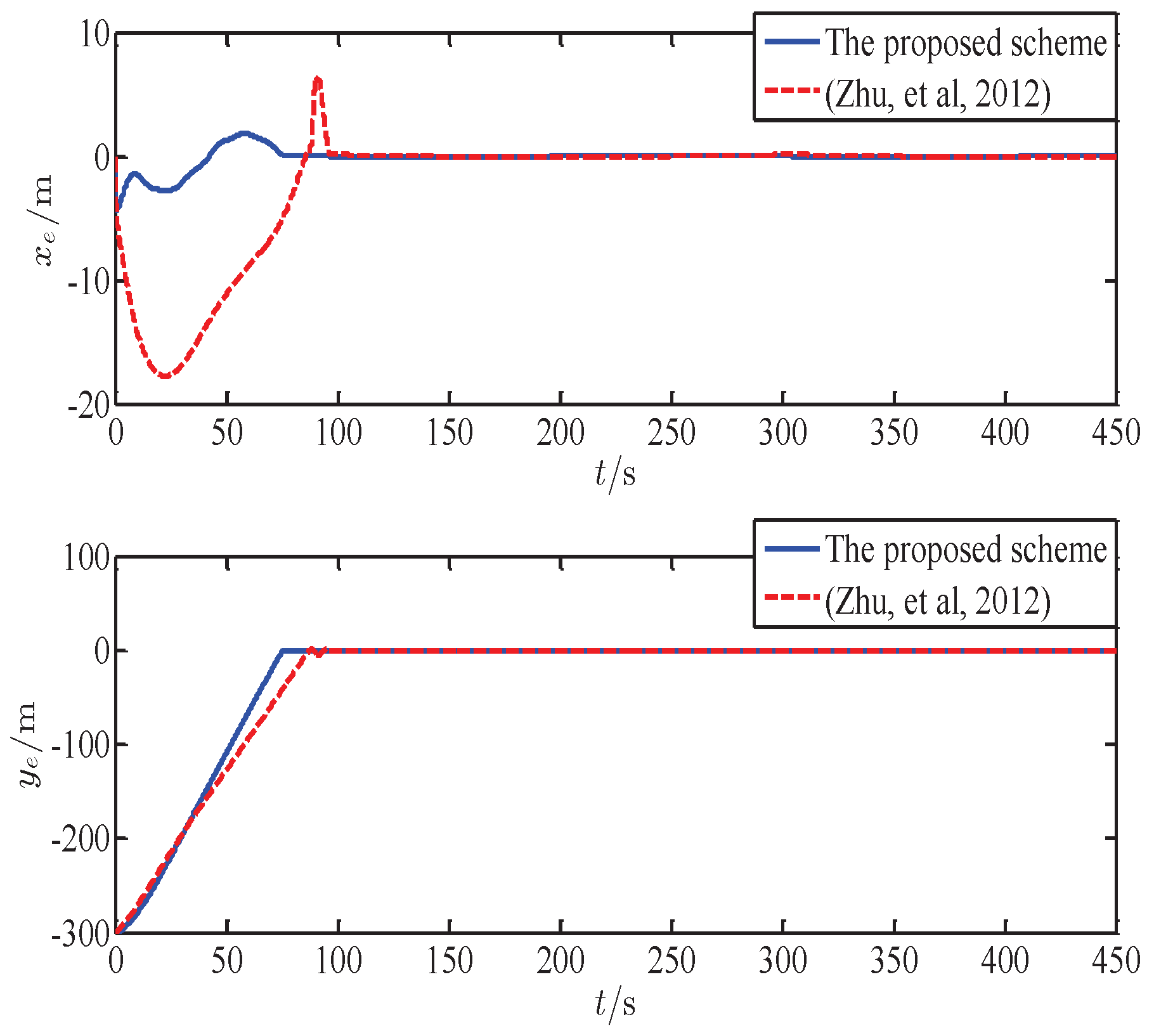
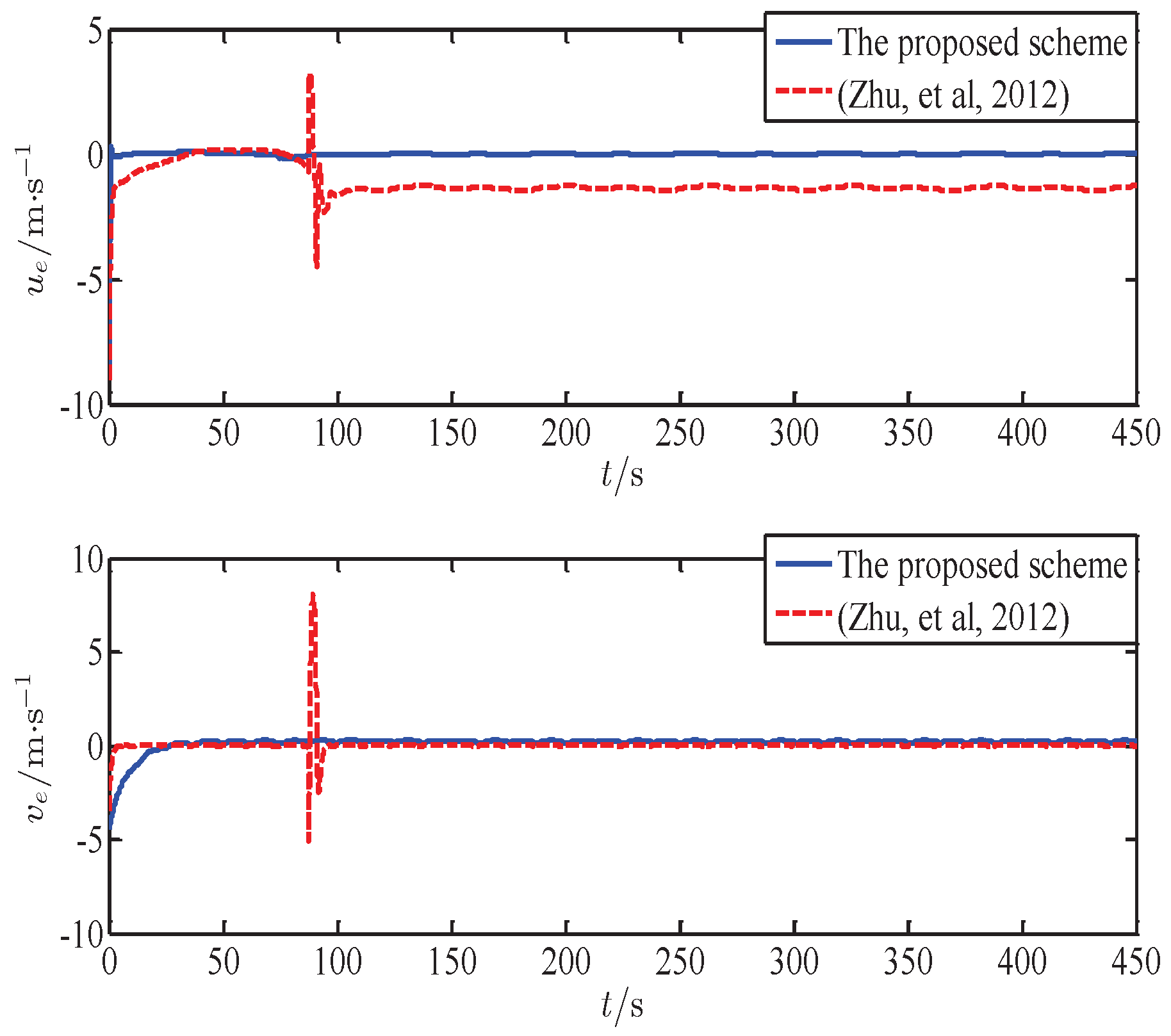
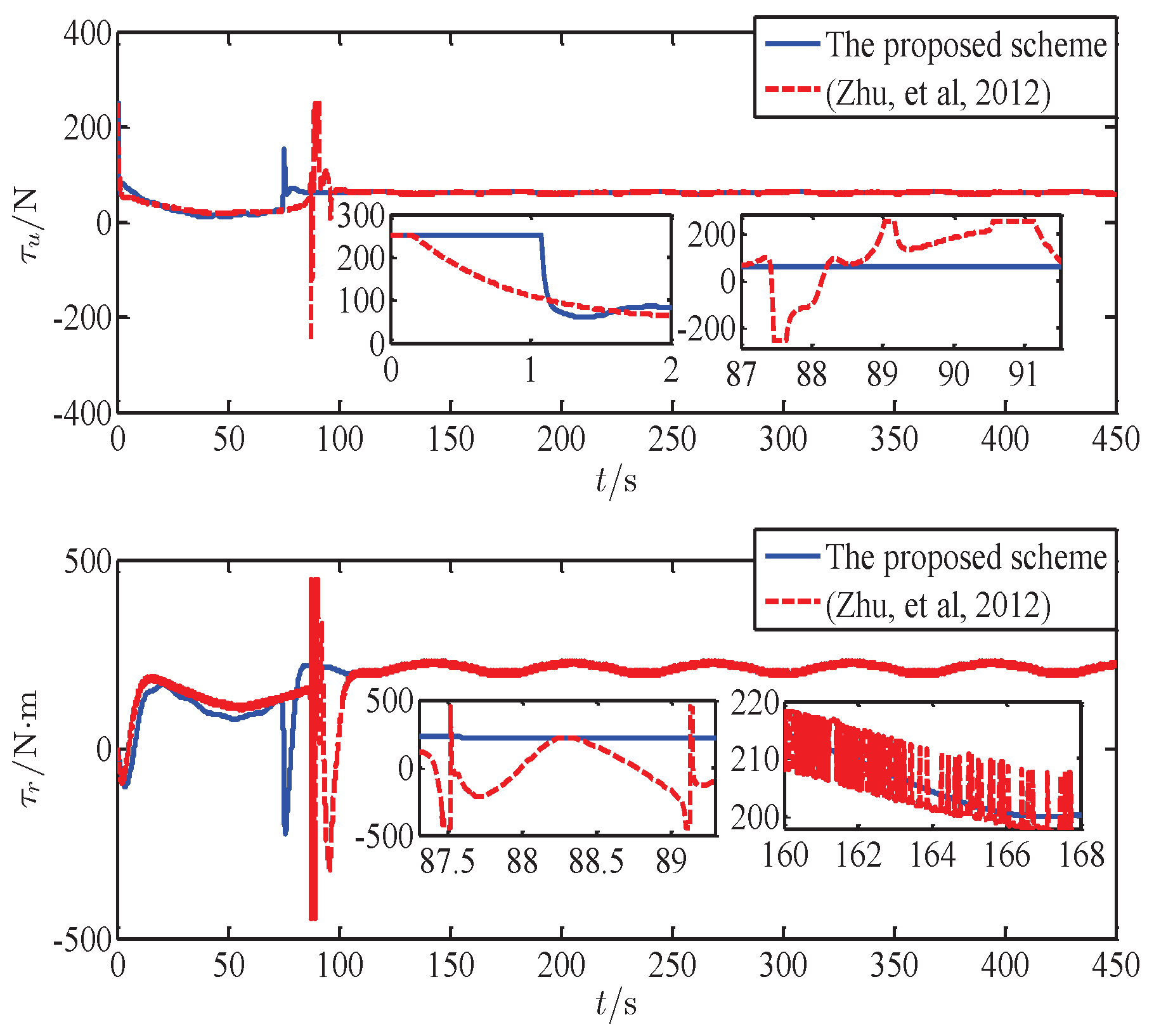
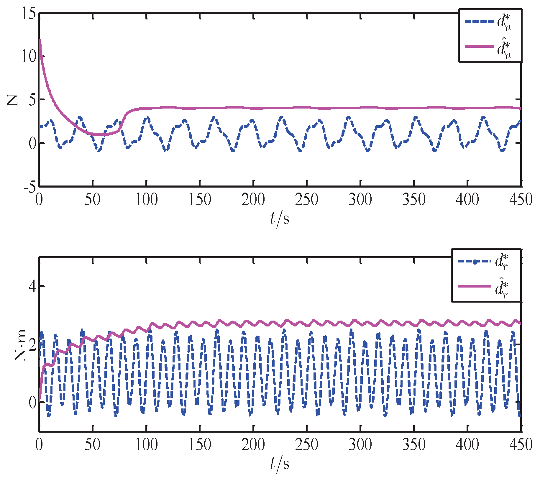
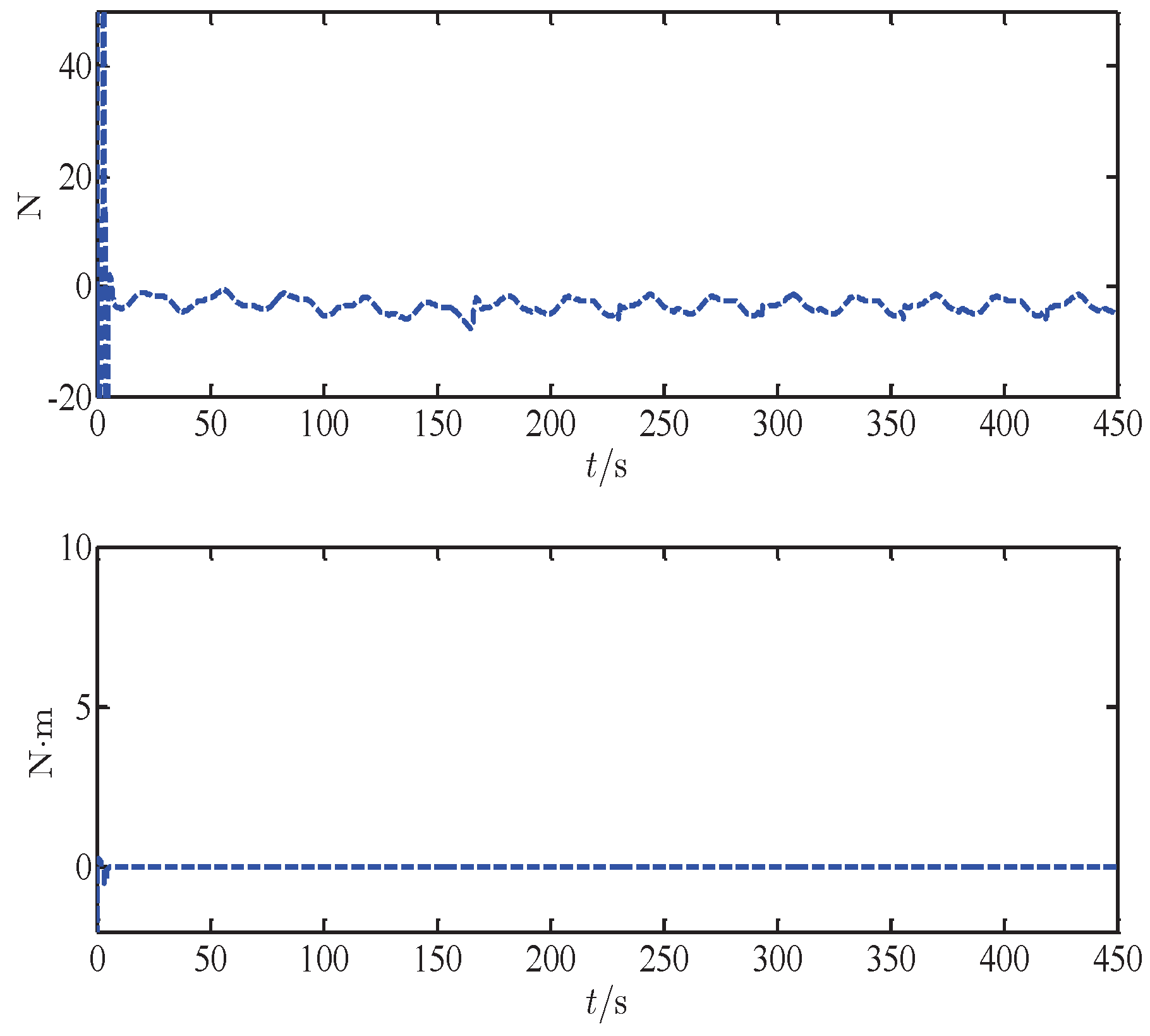
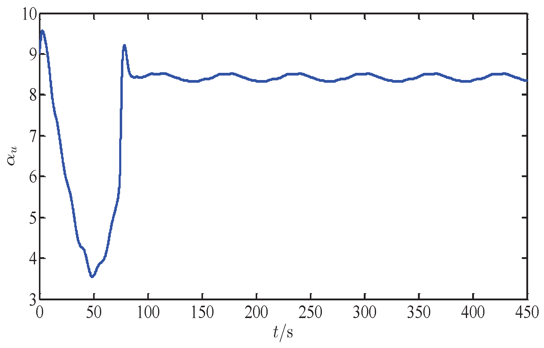
5. Numerical Simulation

In this section, the main purpose is to verify the effectiveness of the proposed method. For the sake of comparison, the proposed scheme is compared with a sliding mode robust controller (Zhu, et al., 2012) [28]. The underactuated USV is selected as a 1:70 CyberShip II [46,47], and the corresponding parameters of the dynamics are described in

Table 1. Parameters of CyberShip II.

Parameters	Value
$m_{11}$	25.8
$m_{22}$	33.8
$m_{33}$	2.76
$d_{11}$	0.72
$d_{22}$	0.8896
$d_{33}$	1.9

. Meanwhile, the control parameters and initial conditions are illustrated in

Table 2. Initial conditions and controller parameters.

Initial Condition	Controller Parameters
$x\left(0\right)=0m$	$A_u=1$, $A_r=1$, ${\tau }_{umax}=250$, ${\tau }_{umin}=-250$
$y\left(0\right)=0m$	${\tau }_{rmax}=450$, ${\tau }_{rmin}=-450$, $K_{\zeta u}=4$, ${\sigma }_u=0.1$
$\psi \left(0\right)=0rad$	$K_{\zeta r}=4$, ${\sigma }_r=0.1$, $\lambda =4.5$, $M=2$, ${\gamma }_1=0.1$
$u\left(0\right)=0m/s$	${\gamma }_2=0.1$, ${\epsilon }_1$= 1, ${\epsilon }_2$ = 0.05, ${\rho }_1$ = 0.1, ${\rho }_2$ = 0.1
$v\left(0\right)=0m/s$	${\mathsf{\Gamma }}_1$ = 2.8, ${\kappa }_1$ = 0.06, ${\mathsf{\Gamma }}_2$ = 2, ${\kappa }_2$ = 0.005, ${\varsigma }_1$ = 10, $d_{u0}^{*}=0.1$
$u\left(0\right)=0rad/s$	${\varphi }_1$ = 0.8, ${\varsigma }_2$ = 5, ${\varphi }_2$ = 0.5, $k_{s1}=1$, $k_{s2}=1$, $d_{r0}^{*}=$ 0.1

.

In the simulation, the desired trajectory is described as $x_d=300sin\left(0.03t\right)$, $y_d=300cos\left(0.03t\right)$, and the unmodeled dynamics are selected as

$$\begin{array}{c}\hfill \left[\begin{array}{c}\Delta f_u\\ \Delta f_v\\ \Delta f_r\end{array}\right]=\left[\begin{array}{c}-0.2d_{11}{u}^2-0.1d_{11}{u}^3\\ -0.2d_{22}{v}^2-0.1d_{22}{v}^3\\ -0.2d_{33}{r}^2-0.1d_{33}{r}^3\end{array}\right]\end{array}$$

(51)

Meanwhile, the time-varying ocean disturbances are chosen as

$$\begin{array}{c}\hfill \left[\begin{array}{c}{d}_u\\ d_v\\ d_r\end{array}\right]=\left[\begin{array}{c}1+1.5sin\left(0.2t\right)+0.5cos\left(0.5t\right)\\ 1+1.2sin\left(0.1t\right)+0.1cos\left(0.4t\right)\\ 1+1.3sin\left(0.5t\right)+0.2cos\left(0.3t\right)\end{array}\right]\end{array}$$

(52)

In addition, in order to further verify the superiority of the proposed controller, MIAC index [27] is hired to quantify the tracking errors $j_e\left(j=x,y\right)$, which can be expressed as

$$\begin{array}{c}\hfill MIAC=\frac{1}{t_f-t_0}{\int }_{t_0}^{t_f}\left|j_e\left(\iota \right)\right|d\iota \end{array}$$

(53)

where $t_f$ represents simulation time.

The simulation results are depicted in Figure 3, Figure 4, Figure 5, Figure 6, Figure 7, Figure 8, Figure 9 and Figure 10, and the performance indices are summarized in

Table 3. Performance index of MIAC.

MIAC	Value
the proposed scheme	$\mathrm{MIA}{\mathrm{C}}_{x_e}=0.318$
	$\mathrm{MIA}{\mathrm{C}}_{y_e}=17.11$
(Zhu, et al., 2012)	$\mathrm{MIA}{\mathrm{C}}_{x_e}=2.259$
	$\mathrm{MIA}{\mathrm{C}}_{y_e}=29.45$

.

Figure 3 shows the simulation results for circular tracking trajectory with the uncertain system dynamics and time-varying ocean disturbances. From Figure 3, it is obvious that two controllers can track the given trajectory accurately. However, the proposed scheme converges faster than that of (Zhu et al., 2012). Figure 4 demonstrates the position tracking results. It is evident that the proposed scheme provides better tracking performance than that of (Zhu, et al., 2012). The results of the tracking errors and the velocity errors are presented in Figure 5 and Figure 6, respectively. As shown in Figure 5 and Figure 6, it is clearly observed that the tracking errors and the velocity errors of the proposed scheme converge to zero quickly and still keep at the balance point. However, the tracking errors and the velocity errors of (Zhu, et al., 2012) have fluctuations and steady-state errors. Figure 7 depicts the control inputs ${\tau }_u$ and ${\tau }_r$ of two controllers. We can see that the surge force ${\tau }_u$ has reached saturation at the beginning. This is mainly because a large gain or differential produces large initial value that exceeds the limit of the propulsion system. However, ${\tau }_u$ and ${\tau }_r$ of (Zhu, et al., 2012) also have the problem of input saturation in the control process, and the moment ${\tau }_r$ has the chattering problem due to saturation function. Figure 8 shows that the designed adaptive law can accurately estimate the bounds of the unknown disturbances. Figure 9 depicts that the approximation errors of neural network converge to zero. In addition, the virtual control law ${\alpha }_u$ is shown in Figure 10, and it is clearly observed that ${\alpha }_u$ is not equal to zero.

From Table 3, we can see that the performance index of the proposed scheme is ${\left[0.318,17.11\right]}^T$, and it is only ${\left[14.08\%,58.09\%\right]}^T$ of (Zhu et al., 2012). Based on the above analysis, in terms of tracking precision, convergence speed and control efforts, the proposed scheme has the best control performance.

6. Conclusions

In this paper, a novel adaptive sliding mode control scheme is developed for tracking control of the underactuated USV. Combining neural network, adaptive technique, auxiliary dynamic system and sliding mode control, a robust adaptive tracking controller is presented subject to the uncertain system dynamics and unknown external disturbances, in which the neural network is used to approximate unmodeled dynamics. In order to get closer to practical engineering, both the unknown disturbances and actuator saturation can be solved by constructing adaptive technique and auxiliary dynamic system, respectively. Meanwhile, a hyperbolic tangent function and neural shunting model are adopted to handle the chattering phenomenon and the differential explosion problem, respectively. In addition, the proposed method is then verified according to computer simulation and compared with another method. In the future, the proposed algorithm can be further improved, and collision and obstacle avoidance may also be considered in control design.

References

1. Liu, Z.; Zhang, Y.; Yu, X.; Yuan, C. Unmanned surface vehicles: An overview of developments and challenges. Annu. Rev. Control. 2016, 41, 71–93. [Google Scholar] [CrossRef]
2. Liu, Y.C.; Bucknall, R. Efficient multi-task allocation and path planning for unmanned surface vehicle in support of ocean operations. Neurocomputing 2018, 275, 1550–1566. [Google Scholar] [CrossRef]
3. Song, R.; Liu, Y.C.; Bucknall, R. A multi-layered fast marching method for unmanned surface vehicle path planning in a time-variant maritime environment. Ocean Eng. 2018, 129, 301–317. [Google Scholar] [CrossRef]
4. Wu, D.; Ren, F.; Qiao, L.; Zhang, W. Active disturbance rejection controller design for dynamically positioned vessels based on adaptive hybrid biogeography-based optimization and differential evolution. ISA Trans. 2018, 78, 56–65. [Google Scholar] [CrossRef] [PubMed]
5. Xiang, X.; Yu, C.; Lapierre, L.; Zhang, J.; Zhang, Q. Survey on fuzzy-logic-based guidance and control of marine surface vehicles and underwater vehicles. Int. J. Fuzzy Syst. 2018, 20, 572–586. [Google Scholar] [CrossRef]
6. Yang, Y.; Du, J.L.; Liu, H.B.; Guo, C.; Abraham, A. A trajectory tracking robust controller of surface vessels with disturbance uncertainties. IEEE Trans. Control Syst. Technol. 2014, 22, 1511–1518. [Google Scholar] [CrossRef]
7. Cheein, F.A.; Scaglia, G. Trajectory tracking controller design for unmanned vehicles: A new methodology. J. Field Rob. 2015, 31, 861–887. [Google Scholar] [CrossRef]
8. Do, K.D. Practical control of underactuated ships. Ocean Eng. 2010, 37, 1111–1119. [Google Scholar] [CrossRef]
9. Dong, Z.; Wang, L.; Li, Y.; Liu, T.; Zhang, G. Trajectory tracking control of underactuated USV based on modified backstepping approach. Int. J. Naval Archit. Ocean Eng. 2015, 7, 817–832. [Google Scholar] [CrossRef] [Green Version]
10. Mu, D.; Wang, G.; Fan, Y. Tracking control of podded propulsion unmanned surface vehicle with unknown dynamics and disturbance under input saturation. Int. J. Control Autom. Syst. 2018, 16, 1905–1915. [Google Scholar] [CrossRef]
11. Mu, D.; Wang, G.; Fan, Y.; Qiu, B.; Sun, X. Adaptive trajectory tracking control for underactuated unmanned surface vehicle subject to unknown dynamics and time-varing disturbances. Appl. Sci. 2018, 4, 547. [Google Scholar] [CrossRef]
12. Serrano, M.E.; Scaglia, G.; Godoy, S.A.; Mut, V.; Ortiz, O.A. Trajectory tracking of underactuated surface vessels: A linear algebra approach. IEEE Trans. Control Syst. Technol. 2014, 22, 1103–1111. [Google Scholar] [CrossRef]
13. Ye, L.Q.; Zong, Q. Tracking control of an underactuated ship by modified dynamic inversion. ISA Trans. 2018, 83, 100–106. [Google Scholar] [CrossRef] [PubMed]
14. Du, H.; Shi, P. A new robust adaptive control method for modified function projective synchronization with unknown bounded parametric uncertainties and external disturbances. Nonl. Dyn. 2016, 85, 355–363. [Google Scholar] [CrossRef]
15. Zhang, G.; Zhang, X. Concise robust adaptive path-following control of underactuated ships using DSC and MLP. IEEE J. Ocean. Eng. 2014, 39, 685–694. [Google Scholar] [CrossRef]
16. Liu, Y.J.; Gao, Y.; Tong, S.; Li, Y. Fuzzy approximation-based adaptive backstepping optimal control for a class of nonlinear discrete-time systems with dead-zone. IEEE Trans. Fuzzy Syst. 2016, 24, 16–28. [Google Scholar] [CrossRef]
17. Utkin, V.I. Sliding Modes in Control and Optimization; Springer-Verlag: Berlin, Germany, 1992. [Google Scholar]
18. Ashrafiuon, H.; Muske, K.R. Sliding mode tracking control of surface vessels. IEEE Trans. Ind. Electron. 2008, 55, 4004–4012. [Google Scholar] [CrossRef]
19. Yu, R.; Zhu, Q.; Xia, G.; Liu, Z. Sliding mode tracking control of an underactuated surface vessel. IET Control Theory Appl. 2012, 6, 461–466. [Google Scholar] [CrossRef]
20. Fahimi, F. Sliding-mode formation control for underactuated surface vessels. IEEE Trans. Rob. 2007, 23, 617–622. [Google Scholar] [CrossRef]
21. Yin, S.; Xiao, B. Tracking control of surface ships with disturbance and uncertainties rejection capability. IEEE ASME Trans. Mech. 2016, 22, 1154–1162. [Google Scholar] [CrossRef]
22. Xu, J.; Wang, M.; Qiao, L. Dynamical sliding mode control for the trajectory tracking of underactuated unmanned underwater vehicles. Ocean Eng. 2015, 105, 54–63. [Google Scholar] [CrossRef]
23. Sun, Z.; Zhang, G.; Qiao, L.; Zhang, W.D. Robust adaptive trajectory tracking control of underactuated surface vessel in fields of marine practice. J. Mar. Sci. Technol. 2015, 10, 1–8. [Google Scholar] [CrossRef]
24. Han, J. From PID to active sisturbance rejection control. IEEE Trans. Ind. Electron. 2009, 56, 900–906. [Google Scholar] [CrossRef]
25. Li, Z.; Sun, J.; Soryeok, O. Design, analysis and experimental validation of a robust nonlinear path following controller for marine surface vessels. Automatica 2009, 45, 1649–1658. [Google Scholar] [CrossRef]
26. He, W.; Dong, Y.; Sun, C. Adaptive neural impedance control of a robotic manipulator with input saturation. IEEE Trans. Syst. Man Cybern. Syst. 2016, 46, 334–344. [Google Scholar] [CrossRef]
27. Zhu, G.B.; Du, J.L. Global robust adaptive trajectory tracking control for surface ships under input saturation. IEEE J. Ocean. Eng. 2018, 1–9. [Google Scholar] [CrossRef]
28. Zhu, Q.D.; Yu, R.T.; Xia, G.H.; Liu, Z.L. Sliding-mode robust tracking control for underactuated surface vessels with parameter uncertainties and external disturbances. Control Theory Appl. 2012, 29, 959–964. [Google Scholar]
29. Chwa, D. Global tracking control of underactuated ships with input and velocity constraints using dynamic surface control method. IEEE Trans. Control Syst. Technol. 2011, 19, 1357–1370. [Google Scholar] [CrossRef]
30. Peng, Z.; Wang, D.; Chen, Z.; Hu, X.; Lan, W. Adaptive dynamic surface control for formations of autonomous surface vehicles with uncertain dynamics. IEEE Trans. Control Syst. Technol. 2013, 21, 513–520. [Google Scholar] [CrossRef]
31. Jin, X. Fault tolerant finite-time leader-follower formation control for autonomous surface vessels with LOS range and angle constraints. Automatica 2016, 68, 228–236. [Google Scholar] [CrossRef]
32. Ros, S.; Roy, S.B.; Kar, I.N. Adaptive-robust control of Euler-Lagrange systems with linearly parametrizable uncertainty bound. IEEE Trans. Control Syst. Technol. 2018, 26, 1842–1850. [Google Scholar]
33. Anastassiou, G.A. Fractional neural network approximation. Comput. Math. Appl. 2012, 64, 1655–1676. [Google Scholar] [CrossRef] [Green Version]
34. Zheng, Z.W.; Zou, Y. Adaptive integral LOS path following for an unmanned airship with uncertainties based on robust RBFNN backstepping. ISA Trans. 2016, 65, 210–219. [Google Scholar] [CrossRef]
35. Mu, D.; Wang, G.; Fan, Y.; Sun, X.; Qiu, B. Adaptive LOS path following for a podded propulsion unmanned surface vehicle with uncertainty of model and actuator saturation. Appl. Sci. 2017, 12, 1232. [Google Scholar] [CrossRef]
36. Zhu, G.B.; Du, J.L.; Kao, Y.G. Command filtered robust adaptive NN control for a class of uncertain strict-feedback nonlinear systems under input saturation. IEEE Trans. Cybern. 2018, 355, 7548–7569. [Google Scholar] [CrossRef]
37. Niu, B.; Li, H.; Zhang, Z.Q.; Li, J.Q.; Hayat, T.; Alsaadi, F.E. Adaptive neural-network-based dynamic surface control for stochastic interconnected nonlinear nonstrict-feedback systems with dead zone. IEEE Trans. Syst. Man Cybern. Syst. 2018, 1–13. [Google Scholar] [CrossRef]
38. Niu, B.; Wang, D.; Alotaibi, N.D.; Alsaadi, F.E. Adaptive neural state feedback tracking control of stochastic nonlinear switched systems: An average dwell-time method. IEEE Trans. Neural Netw. Learn. Syst. 2018, 30, 1076–1087. [Google Scholar] [CrossRef]
39. He, W.; Yin, Z.; Sun, C. Adaptive neural network control of a marine vessel with constraints using the asymmetric barrier Lyapunov function. IEEE Trans. Cybern. 2017, 47, 1641–1651. [Google Scholar] [CrossRef]
40. Yang, S.X.; Meng, M. An efficient neural network approach to dynamic robot motion planning. IEEE Trans. Cybern. 2000, 13, 143–148. [Google Scholar] [CrossRef]
41. Yang, S.X.; Zhu, A.; Yuan, G.F.; Meng, M. A bioinspired neurodynamics-based approach to tracking control of mobile robots. IEEE Trans. Ind. Electron. 2012, 59, 3211–3220. [Google Scholar] [CrossRef]
42. Qu, H.; Yang, S.X.; Willms, A.R.; Zhang, Y. Real-time robot path planning based on a modified pulse-coupled neural network model. IEEE Trans. Neural Netw. 2009, 20, 1724–1739. [Google Scholar] [PubMed]
43. Chen, M.; Ge, S.S.; Ren, B.B. Adaptive tracking control of uncertain MIMO nonlinear systems with input constraints. Automatica 2011, 47, 452–465. [Google Scholar] [CrossRef]
44. Du, J.L.; Hu, X.; Krstic, M.; Sun, Y.Q. Robust dynamic positioning of ships with disturbances under input saturation. Automatica 2016, 73, 207–214. [Google Scholar] [CrossRef]
45. Polycarpou, M.M. Fault accommodation of a class of multivariable nonlinear dynamical systems using a learning approach. IEEE Trans. Autom. Control 2001, 46, 736–742. [Google Scholar] [CrossRef]
46. Dai, S.L.; Wang, C.; Luo, F. Identification and learning control of ocean surface ship using neural networks. IEEE Trans. Ind. Inf. 2012, 8, 801–810. [Google Scholar] [CrossRef]
47. Pan, C.Z.; Lai, X.Z.; Yang, S.X.; Wu, M. An efficient neural network approach to tracking control of an autonomous surface vehicle with unknown dynamics. Expert Syst. Appl. 2013, 40, 1629–1635. [Google Scholar] [CrossRef]
Figure 1. The earth-fixed inertial and the body-fixed frame.
Applsci 09 01240 g001
Figure 2. The structure of the proposed adaptive sliding mode control scheme for the underactuated USV.
Applsci 09 01240 g002
Figure 3. Tracking performance results of circular trajectory.
Applsci 09 01240 g003
Figure 4. Position tracking results of circular trajectory.
Applsci 09 01240 g004
Figure 5. Tracking errors results of circular trajectory.
Applsci 09 01240 g005
Figure 6. Velocity errors results of circular trajectory.
Applsci 09 01240 g006
Figure 7. Control inputs of circular trajectory.
Applsci 09 01240 g007
Figure 8. Disturbances and their bound estimates.
Applsci 09 01240 g008
Figure 9. Approximation error results of neural network.
Applsci 09 01240 g009
Figure 10. Virtual control law α u .
Applsci 09 01240 g010