Article

Improved Visible Light-Based Indoor Positioning System Using Machine Learning Classification and Regression

Robotics and Mechatronics Lab, University of Ulsan, Ulsan 44610, Korea
*
Author to whom correspondence should be addressed.
Appl. Sci. 2019, 9(6), 1048; https://doi.org/10.3390/app9061048
Submission received: 11 February 2019 / Revised: 6 March 2019 / Accepted: 7 March 2019 / Published: 13 March 2019
(This article belongs to the Special Issue Light Communication: Latest Advances and Prospects)

Abstract

:
Recently, indoor positioning systems have attracted a great deal of research attention, as they have a variety of applications in the fields of science and industry. In this study, we propose an innovative and easily implemented solution for indoor positioning. The solution is based on an indoor visible light positioning system and dual-function machine learning (ML) algorithms. Our solution increases positioning accuracy under the negative effect of multipath reflections and decreases the computational time for ML algorithms. Initially, we perform a noise reduction process to eliminate low-intensity reflective signals and minimize noise. Then, we divide the floor of the room into two separate areas using the ML classification function. This significantly reduces the computational time and partially improves the positioning accuracy of our system. Finally, the regression function of those ML algorithms is applied to predict the location of the optical receiver. By using extensive computer simulations, we have demonstrated that the execution time required by certain dual-function algorithms to determine indoor positioning is decreased after area division and noise reduction have been applied. In the best case, the proposed solution took 78.26% less time and provided a 52.55% improvement in positioning accuracy.

1. Introduction

In 2007, the Visible Light Communication (VLC) standards CP-1221 (VLC system) and CP-1222 (Visible Light ID system) were established by the Japan Electronics and Information Technology Industries Association (JEITA). CP-1222 is a standard concerned with the field of visible light positioning (VLP) [1]. In addition to the standards that came from Japan, the IEEE Standards Association has published IEEE 802.15.7: Visible Light Communication: Modulation Schemes and Dimming Support [2], and IEEE 802.15.7-2018—IEEE Draft Standard for Local and Metropolitan Area Networks—Part 15.7: Short-Range Optical Wireless Communications [3]. Standardization in VLC may be the catalyst for technological innovation and product commercialization in the near future.
VLC-based indoor positioning provides opportunities to develop highly reliable, robust, and inexpensive positioning technologies [4]. Philips, one of the largest electronics companies in the world, has achieved some initial success in this field. Their solution is to embed Light Emitting Diode (LED) luminaires with VLC technology, and utilize the store lighting to provide location data using the store’s mobile app [5]. Additional VLP applications, such as mobile robots, assistive devices for patients with impaired vision or other handicaps are being studied [6,7,8].
The Global Positioning System (GPS) is the perfect choice for outdoor applications because of its coverage and cost [9]. For indoor positioning, there are several possible options, including WiFi [10,11], Zigbee-based internet of things (IoT) [12], Bluetooth [13], radio frequency identification (RFID) [14], and camera-based solutions [15]. Depending on many factors, each option achieves a different level of accuracy, but the applied algorithms can be considered a fundamental factor. In this article, we examine some of the indoor positioning studies utilizing machine learning (ML) algorithms, which play a key role in our proposed solution. First, indoor WiFi localization is always the preferred choice, because of the universality of WiFi signals and the availability of many wearable devices with WiFi signal receivers [10]. Akram et al. [11] proposed a novel hybrid indoor WiFi localization that combined soft clustering with the random decision forest algorithm. Zan Li et al. [12] used another ML approach that was applied to the ZigBee-based IoT network. These authors investigated a narrow-band indoor positioning system (IPS) fusing time and received signal strength via ensemble learning. Using a random forest regression model, their solution achieved a 36.1% improvement over the traditional method based on received signal strengths (RSS). For RFID technology, the application of ML to locate an object position in the indoor environment is also efficacious. In Reference [14], to overcome the limitation of the mutual dependence of positioning accuracy and the density of reference tags, an extreme ML algorithm was adopted. The results showed that their solution created a better performance than existing solutions. In addition to using device-based localization systems, there is also the option of using device-free localization (DFL) in a wireless sensor network field to locate a person. In this innovative approach, the application of ML to optimize positioning quality is an inevitable trend. The logistic regression classifier has been used to improve the localization accuracy of a fingerprint-based DFL in a changing environment [16], and an extreme ML algorithm with parameterized geometrical feature extraction for DFL is also suggested in Reference [17].
Several recent studies in the field of VLC-based IPS have applied traditional methods as well as improved ML algorithms for better positioning efficiency [18,19,20,21]. Xiansheng Guo et al. [18] proposed an indoor localization solution based on the fusion of multiple classifiers (grid-independent least squares and grid-dependent least squares). This solution produced remarkable results, and obtained 93.03% and 93.15% improvement, respectively, over the RSS ratio and RSS matching methods. Besides reducing positioning errors, the analysis and optimization of other parameters, such as the receiver angle [19] and the LED-ID detection accuracy [20], also contribute significantly to the quality of the system, especially when carried out with the support of ML. However, the influence of reflected waves and noises has not been deeply concerned in these articles. In our previous work [21], the detrimental effects of reflected waves on the VLC-based positioning accuracy as well as incomplete solutions in recent studies have been analyzed in great detail. From this constraint, we proposed a novel method (using kNN-RF) to decrease positioning error in the areas outside the center in the multipath reflection environment without signal pre-processing. We also utilized the importance rate function to reduce computational time, but we found that if we removed too many features in an effort to minimize execution time, the positioning accuracy was reduced.
In this article, to achieve a much higher positioning accuracy and faster computational time under the negative influence of multipath reflection and noises, we suggest an innovative indoor positioning solution. This solution is based on the signal pre-processing technique and dual-function ML algorithms that contain machine learning classification (MLC) and machine learning regression (MLR) functions. The algorithms used were support vector machine (SVM), decision tree (DT), random forest (RF), and k-nearest neighbors (kNN). The obtained results proved that the proposed technique can produce the mean positioning accuracy of 8.75 cm with SVM compared to 19.3 cm with kNN-RF in our previous work [21]. Depending on the selected algorithm, the CPU time also showed a significant improvement with 78.26% in the best case. The encouraging results can be applied to many different indoor environments, from public places (such as supermarkets, theaters, museums, and shopping centers) to private places (such as factories and warehouses). In addition, VLC-based positioning systems can be used for smart home applications and can be used in conjunction with smart canes and smart wheelchairs [8,21]. VLC-based positioning systems can be used to locate the current position of a person carrying an optical sensor, and to help them determine the route to their destination inside a building. Obviously, applications with VLP using the proposed method are very diverse and useful in the world today.
The main features of our solution can be summarized as follows:
  • We first performed noise reduction by using outlier and average filtering. These processes include noise filtering and elimination of low-intensity reflected signals. This type of signal pre-processing improves the accuracy of the later position estimation process.
  • Then these data were classified using the classification function of ML algorithms. Data points were assigned to one of two areas: the center area or the edge area. The area division was based on the correlation between the actual location of the receiver on the floor and the RSS from four groups of LED lights suspended from the ceiling. Data division by region is a unique idea that not only significantly reduces total execution time but also contributes to the improvement in positioning accuracy, due to the signal integrity within each individual area.
  • After noise reduction and area division, the regression function of the ML algorithms was used to predict the location of the receiver. The results show that the proposed solution greatly improved the execution time and positioning accuracy, despite being influenced by many adverse factors, including noises and reflected waves.
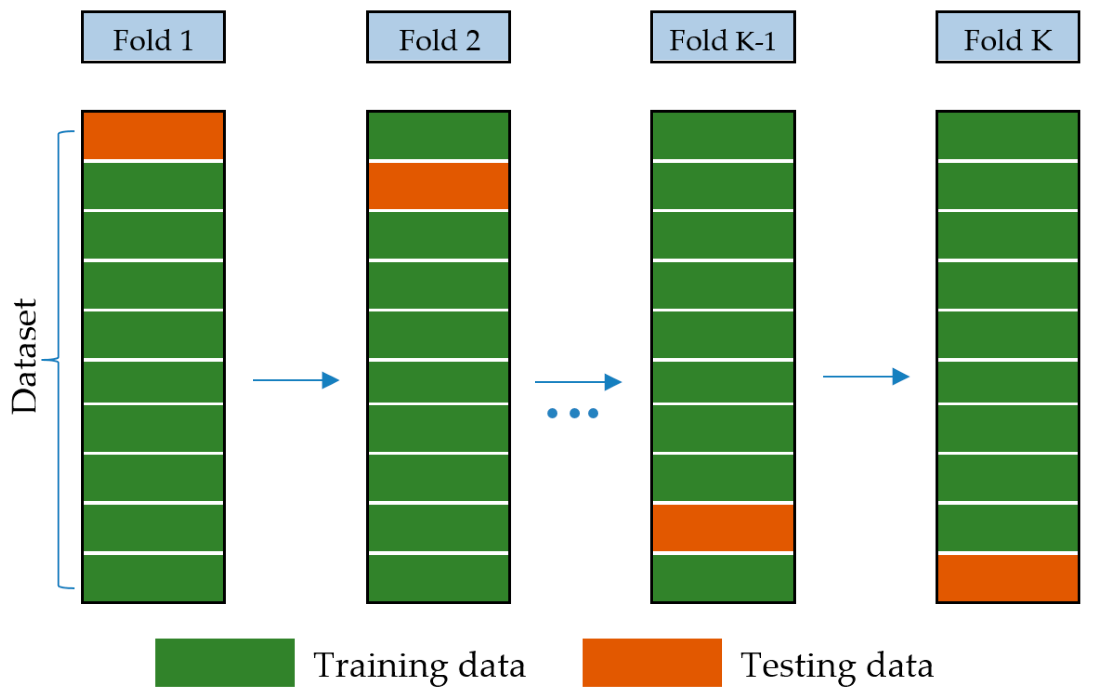
  • To evaluate the effectiveness of each ML algorithm, we compared their accuracy in both in the classification process and the regression process after the Cross-Validation (CV) technique was employed to verify the reliability of the algorithm and avoid overfitting. The comparison of positioning accuracy and computational time for all the methods provides a basis for selecting the optimal algorithm for future research.
In the remainder of the article, the proposed system is presented in Section 2. Then, our proposed solution including noise reduction, area division, and location prediction using dual-function ML algorithms are shown in Section 3. In Section 4, we find the optimal parameters for each algorithm. Section 5 offers the simulation performance, some discussions and the comparisons of some popular ML algorithms in terms of computational time and the positioning accuracy. Finally, the conclusion is considered in Section 6.

2. Proposed System

2.1. Simulation Configuration

To analyze the performance of the proposed solution, a typical empty room (5 m × 5 m × 2.5 m) was assumed, as depicted in Figure 1 [22]. We assumed that there were four LED bulbs suspended from the ceiling at a height of 2.5 m. The total transmitted optical power per LED bulb was fixed at 25 W. The semi-angle of each LED group and the field-of-view (FOV) angle of the photo-detector (PD) were both set at 70°. The four walls were made from plaster that had a reflective rate of 0.7–0.85 [23]. Other important parameters are represented in detail in Table 1.
The technique of RSS-based positioning is often used for indoor positioning because of its simplicity [24]. For this work, we develop our solution based on the RSS and fingerprints. We gathered the input data from each reference fingerprint. The distance between adjacent fingerprints was 20 cm, and a 26 × 26 fingerprint grid was assigned to the floor surface corresponding to 676 reference points. The original coordinates and the fingerprints distribution are shown in Figure 2.

2.2. Simulation Configuration VLC Channel and Signal-To-Noise Ratio (SNR) Analysis

To locate the current position of the PD, the intensity of the light source from each LED was modulated, then multiplexing protocol was used to correctly transmit this data from all LED lights to the PD. Finally, demodulating process was executed at the optical receiver [8]. In this paper, an On-Off keying (OOK) modulation using Manchester encoding and Time-division multiplexing (TDM) protocol were used as shown in Figure 3. By using OOK modulation, the logic ‘1’ corresponds to the light ‘ON’ state, and the logic ‘0’ corresponds to the light ‘OFF’ state. To send an equal number of positive and negative pulses, Manchester encoding was proposed. After encoding the data, each LED signal was sent to the PD at each time slot by TDM protocol, which divided the overall time into many slots [8].
Depending on the structure of the VLC channel, the RSS and SNR values can be changed. In this work, we analyzed both the line-of-sight (LOS) channel and the diffuse channel. In addition, the influence of multiple noises of the system, including shot noise and thermal noise, was considered in detail. For the direct channel, the DC channel gain is given by the following equation [25]:
H L O S = { ( n + 1 2 π ) ( A l 2 ) cos n ( ϕ ) T s ( Ψ d ) g ( Ψ d ) cos ( Ψ ) , 0 Ψ d F O V 0 , Ψ d > F O V ,
where n is the Lambertian order; A is the active detector area of the PD; l is the distance between the LED and the PD; ϕ is the irradiance angle; Ψ d is the incidence angle of the directed channel; Ts( Ψ d ) is the gain of the optical filter; g( Ψ d ) is the gain of the optical concentrator; and FOV is the field of view of the PD.
For simplicity, we focus on the effect of the first reflection signal, because other reflected waves have a negligible effect [21]. Thus, the DC channel gain of the first reflection is computed as follows [25]:
H N L O S = { ( n + 1 2 π ) ( A l 1 2 l 2 2 ) ρ cos n ( ϕ ) d A r e f cos ( λ ) cos ( γ ) cos ( Ψ r ) T s ( Ψ r ) g ( Ψ r ) , 0 Ψ r F O V 0 , Ψ r > F O V ,
where l1 is the distance between an LED and a reflective point; l2 is the distance from a reflective point to the PD; ρ is the reflectance factor; dAref is the reflective element on the wall; λ is the angle of irradiance from an LED group to the reflective point; γ is the angle between a reflective point and the PD; and Ψr is the incidence angle from the wall.
After calculating the DC gain for both direct and diffuse channels, the total received optical power at the PD is as follows [25]:
P T o t a l = 1 4 P T ( H L O S + H N L O S ) ,
where PT is the total transmitting optical power.
To compute the SNR, we first determine the Gaussian noise from the output, which is the sum of shot noise σ S 2 , thermal noise σ T 2 , and inter-symbol interference σ I S I 2 . However, the σ I S I 2 term can be removed, due to short transmitting duration. The total noise can be expressed as [22]:
N t o t a l 2 = σ S 2 + σ T 2 .
Assumed that the dark current noise is small, the shot noise variance due to the received signal and the background radiation is given by [22]:
σ S 2 = 2 q R P T o t a l B + 2 q I B I 2 B ,
where q is the electronic charge; R is the PD responsibility; I B is the photocurrent due to background radiation; I 2 is the noise bandwidth factor; and B is the equivalent noise-bandwidth of the PD.
The thermal noise variance is given by [22]:
σ T 2 = 8 π κ T k G η P D A I 2 B 2 + 16 π 2 κ T k Γ g η P D 2 A 2 I 3 B 3 ,
where κ is the Boltzmann’s constant; T k is the absolute temperature; G is the open-loop voltage gain; η P D is the fixed capacitance of PD per unit area; Γ is the FET channel noise factor, g is the FET transconductance; and I 3 is the noise-bandwidth factor.
Finally, the SNR for the LOS channel, diffuse channel, and overall channel are depicted in Figure 4, and the SNR equation is as follows [25]:
S N R = R 2 P T o t a l 2 N t o t a l 2 .

3. Proposed Solution

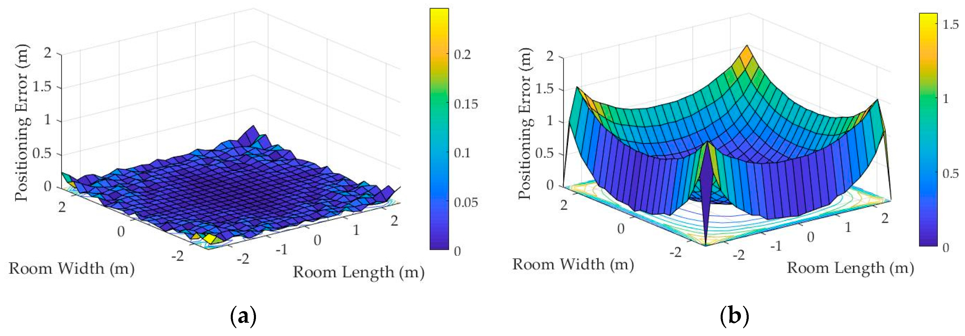
In an optimal environment, traditional indoor positioning solutions can achieve very high accuracy, particularly when the reflected channel is ignored. However, besides the noises due to sunlight and other electric lights, reflection light always exists, and its intensity may vary according to the current position of the receiver. These reflected signals produce a detrimental effect on positioning accuracy [21]. This is clearly shown in Figure 5 when we use a Trilateration algorithm for indoor positioning composed of two completely opposing environments, one side is the environment that only exists as a directed channel (Figure 5a), and one side is the environment including the highest reflection (Figure 5b). Under the negative impact of multipath reflections, the SNR decreases at the corners and the edges, thus the positioning errors are substantially worse when the PD moves away from the room’s center (see Figure 4) [26]. With the maximum error of approximately 1.5 m occurring at the corners, Figure 5b is a vivid illustration of the negative impact of multipath reflections on positioning accuracy. Therefore, VLC-based indoor positioning techniques must take into consideration all types of noise and reflected signals.
In recent years, ML has made great leaps and has achieved outstanding successes in many fields of science, especially in the field of image processing. However, the application of ML for VLC-based IPS has been quite limited. Challenges when using ML for this application, including sensitivity to noise and high computational times [27], can be considered underlying causes.
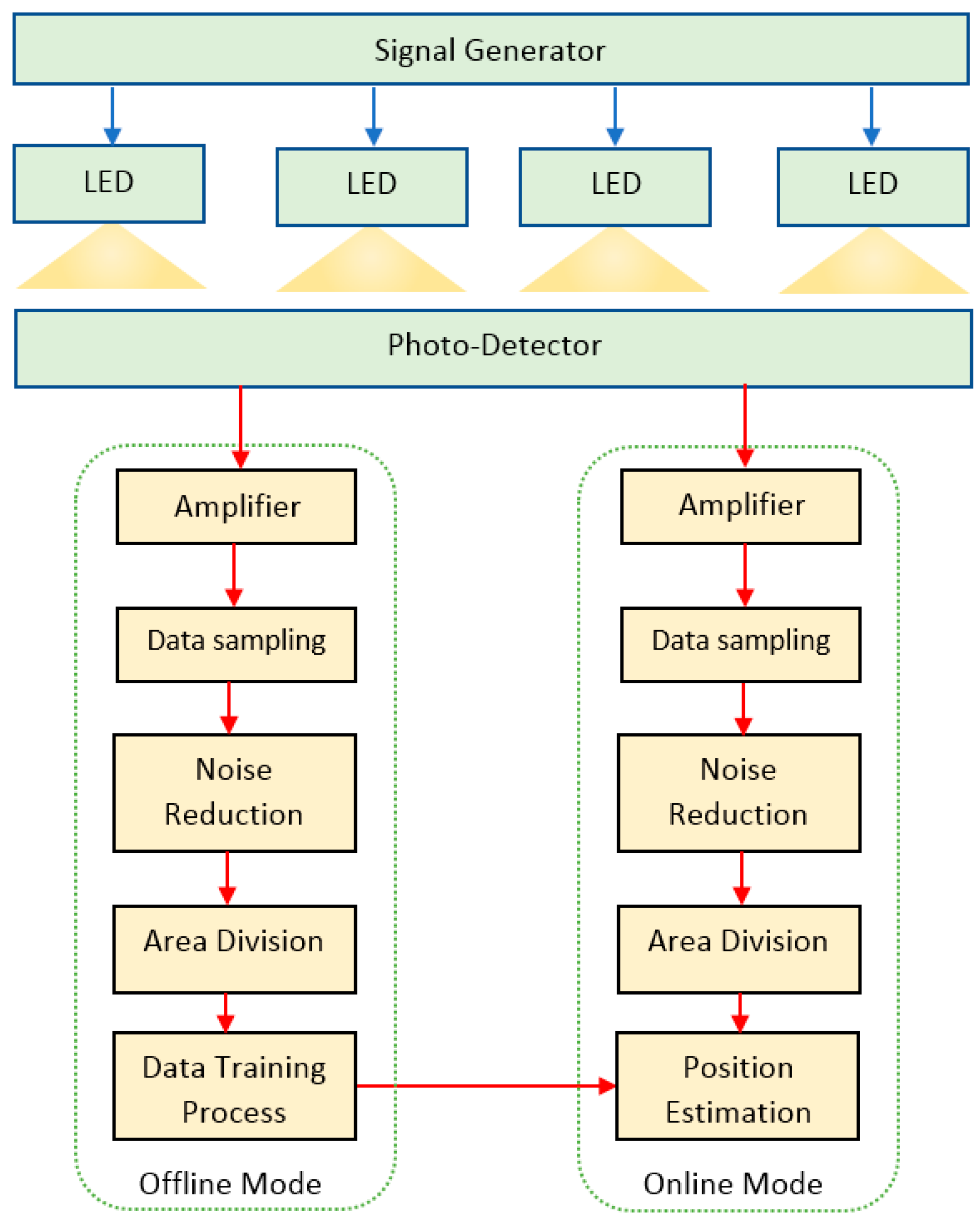
From the above discussion, we propose an effective solution for VLC-based indoor positioning that improves not only the positioning accuracy but also the execution time (Figure 6). To deal with those two parameters, we combine signal pre-processing techniques and two popular functions of ML-based algorithms (the classification function and the regression function). Signal pre-processing helps filter the noise and eliminates low-intensity reflective signals, thereby reducing the sensitivity to noise. This creates a basis for more accurate positioning later. Then, the two classification and regression functions, in turn, are carried out. The classification process plays a key role in reducing the computational time by dividing the floor surface into two isolated areas, and the regression process helps determine the estimated location of the PD. The whole process is divided into two distinct modes: offline mode and online mode. The main tasks of the offline mode are to collect the RSS from all fingerprints, then in turn conduct noise reduction, area division, and training process. While the online mode gathers online data from the current location of the PD, then the same processes of noise reduction and area division are taken place. However, the difference happens in the final step, when the online mode uses training data in the offline mode to predict the current location of the PD. Further details are discussed in the following Sections.

3.1. Low-Intensity Reflected Signal Elimination and Noise Reduction

With the LOS channel, the time it takes for the PD to receive the optical signal depends on the distance between the LED light and the PD. With the diffuse channel, it depends on the position of the PD in relation to the reflective point on the wall. At any particular time, the signal received by the PD may be a directed signal from an LED, or a non-directed signal from one of the four walls. The intensity of the reflected signal depends on the position of the receiver as well as the reflective rate of the wall [23]. In Reference [28], to eliminate the diffuse signals, the strongest waves collection was conducted, which can help reduce the impact of multipath reflections. However, in some cases, a combination of a very high reflective rate and other noise sources (i.e., thermal noise and shot noise) can cause the highest signals received at some locations to be diffuse signals. We describe some popular ML algorithms used for area division and location prediction in the next two Sections, while noise sensitivity is a major weakness of ML. It is clear that noise reduction and the elimination of low-intensity reflected signals are important signal pre-processing steps for improving positioning quality. To accomplish this, the following steps were taken:
Step 1: Low Reflected Optical Power Elimination
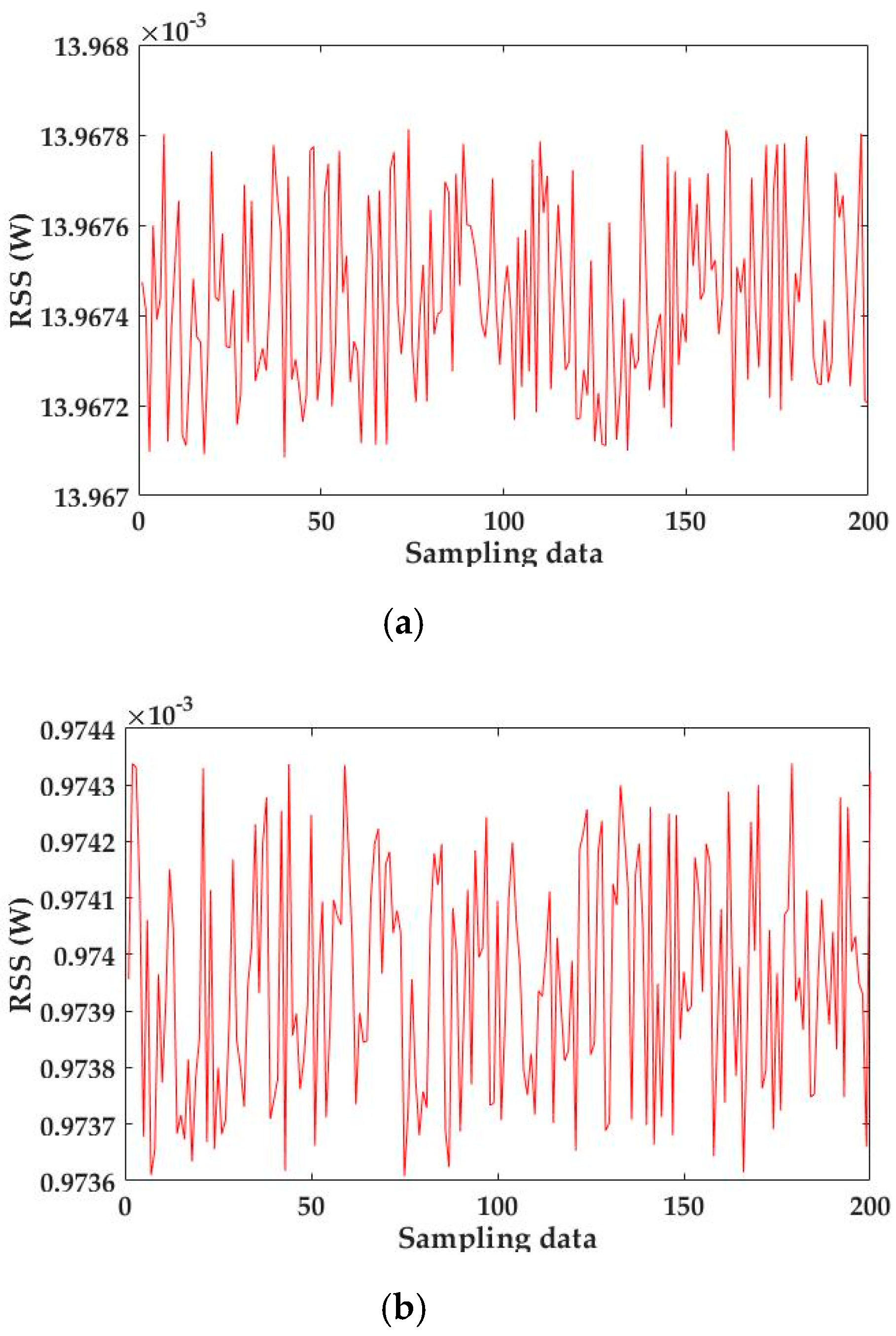
The received signal from the LED light can be either an LOS signal or a diffuse signal, and this happens randomly according to each sampling. As shown in Figure 7, there is a great difference between the intensity of direct signals and reflected signals at a random point on the floor. If the reflected signal has a very small power compared to direct signals, the training data is no longer uniform. Therefore, eliminating these signal types an important step. To implement this, we calculated the mean value of the RSS based on N sampling data using the following equation:
R S S ¯ = i = 1 N R S S i N .
Next, we used the outlier RSS filter to remove the signals whose power magnitudes are significantly different from the other signals [12]:
R S S i > ( 1 + α ) R S S ¯ ,
where α is the outlier ratio and is set to 0.2 in our work after evaluating many different values (α > 0).
Step 2: Noise Reduction with Moving Average Filter
After removing the low power reflected signals, we continued to optimize the signals by eliminating the other noise types (i.e., thermal noise and shot noise), which are known as Gaussian noises due to the sunlight from a window or an entrance door [29]. In this Section, we proposed a very simple noise reduction technique called moving average filter [30]. In some cases, this method may not achieve high efficiency if the signal and noise distribution are related to each other [31]. However, in VLC case, the thermal noise and shot noise are signal-independent Gaussian noises [32] and the sum of these random noises is zero in any phase of signal. This filter uses the current and previous K − 1 samples to calculate the average RSS:
R S S n e w [ n ] = 1 K l = 0 K 1 R S S [ n l ] .
After performing this averaging process, the results were utilized as the training dataset for the next steps. The effectiveness of this method is analyzed in detail in Section 5, by comparing cases before and after noise removal.

3.2. Area Division with MLC

As discussed in 
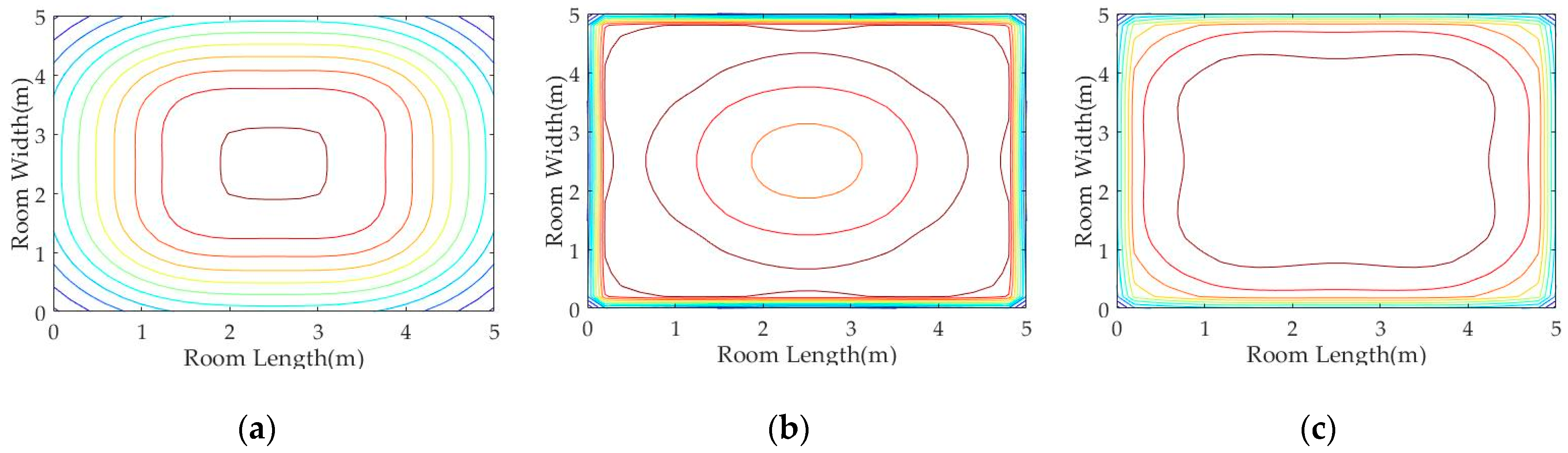
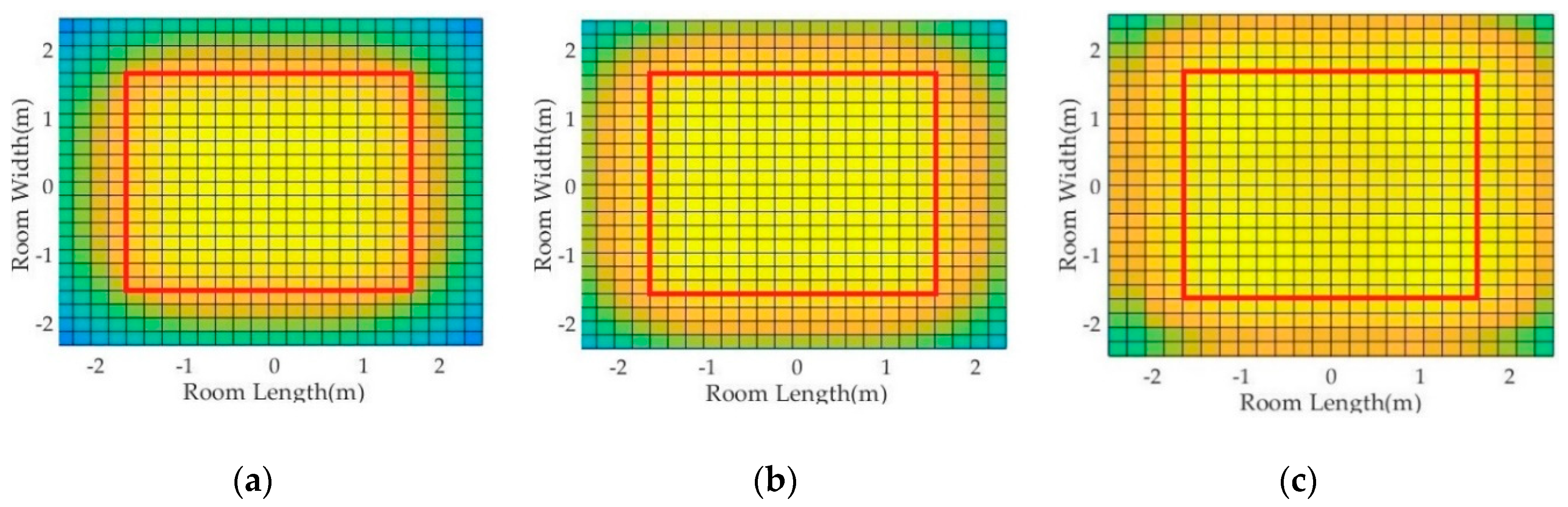
Section 1, computational time is a major constraint when using ML algorithms. In this study, we utilized the classification function of ML to reduce the effect of run time on system performance. This solution is based on the heterogeneous distribution of the SNR (Figure 4). In Figure 4a, the shape of the signal is uniform across the entire floor thanks to the elimination of reflected noise. This homogenous state, however, disappears when the received signal at the PD is a combination of directed and non-directed optical signals (Figure 4c). To conduct area division, we divided the floor of the room into two sections: a center area and an edge area (corners and near-the-wall areas). To prepare for collecting the training dataset, the boundary between the two areas can be determined by two important factors: the identity of the received optical power and the amount of data used for the training process.
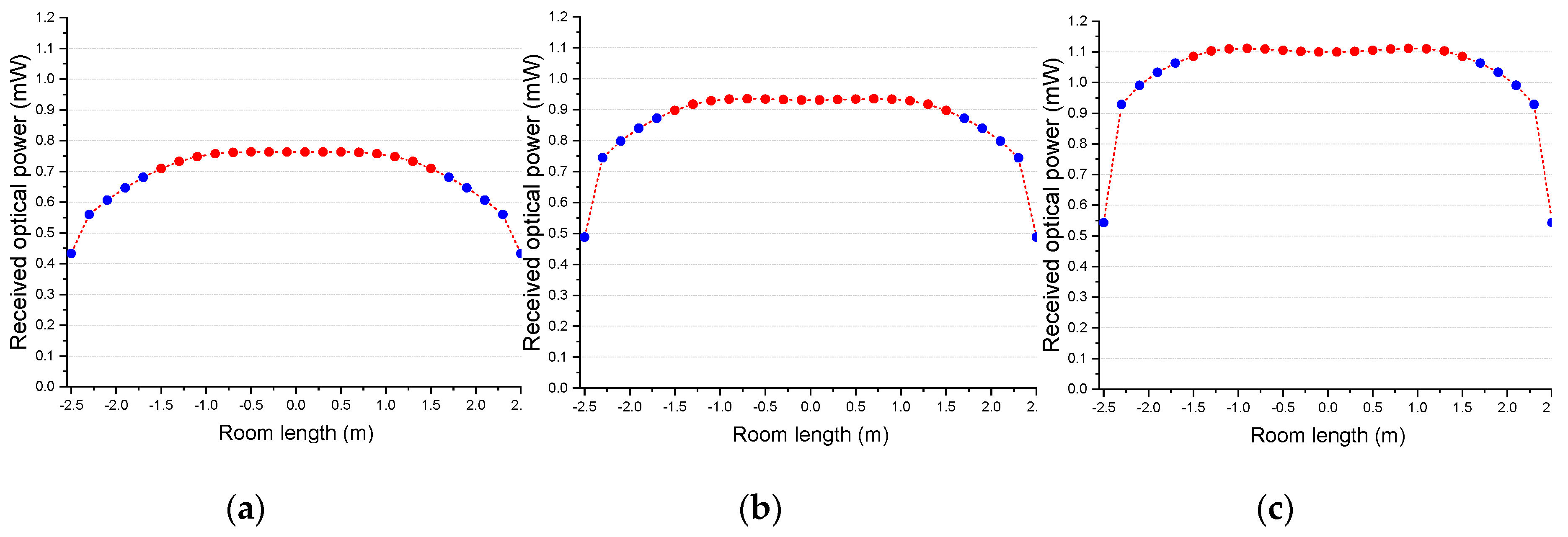
Figure 8 shows the average power distribution according to the vertical projection of the room in three reflection level cases: 0.2, 0.5, and 0.8. These values depend directly on the surface material used for the walls, which cause reflective noises [23]. There is a significant difference in the power distribution between the central area (with red spots) and the edge area (with blue spots). It is clear that the central area has a more uniform distribution and is more stable than the edge area, which shows greater reflection intensity.
To ensure similarity in the amount of training data for the two areas, we set the boundary as shown in Figure 9. By using this division, the training data in the center area and the edge area accounted for 47.93% and 52.07%, respectively, of the total 676 reference points. This balance in the amount of training data helped to reliably assess the effectiveness of the classification process.
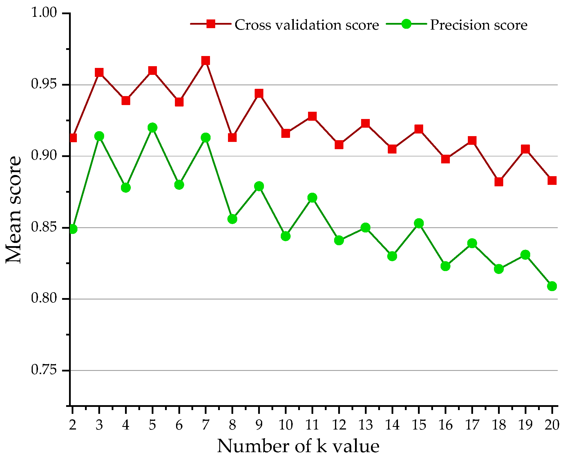
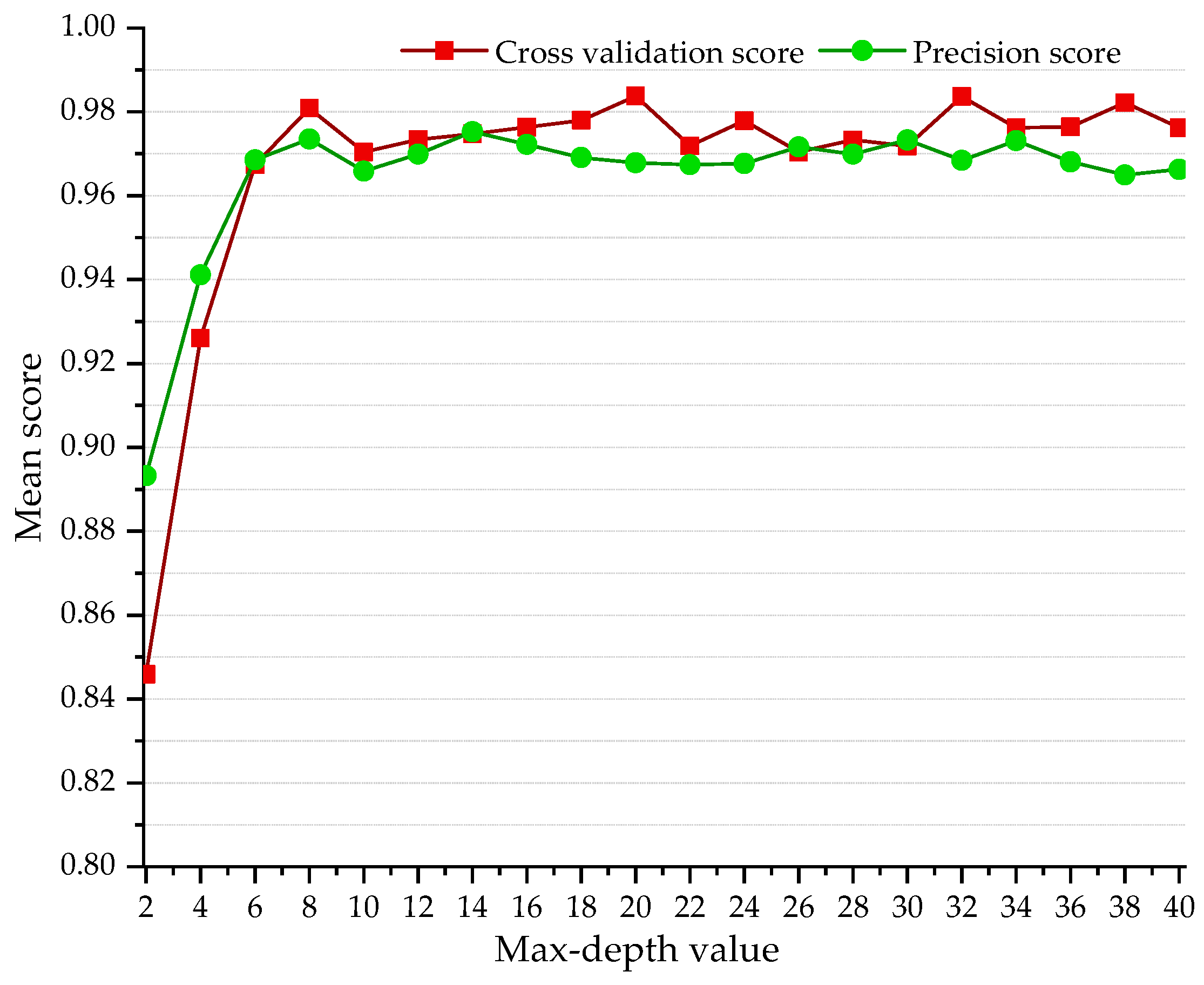
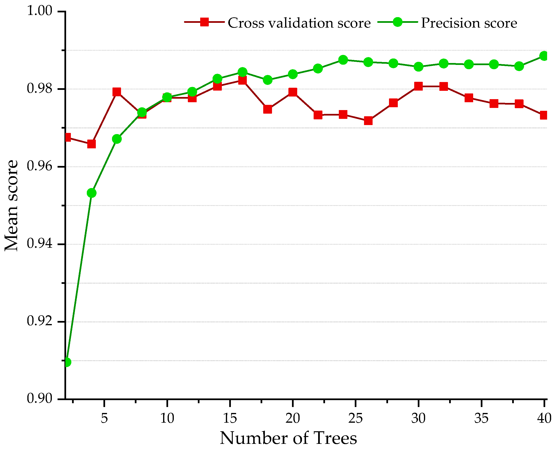
In this study, we used the SVM, DT, kNN, and RF ML algorithms, due to their ability to both classify and regress. After the training and prediction process, we calculated the accuracy score and conducted K-fold CV to evaluate the robustness of each method.

3.3. Location Prediction with MLR

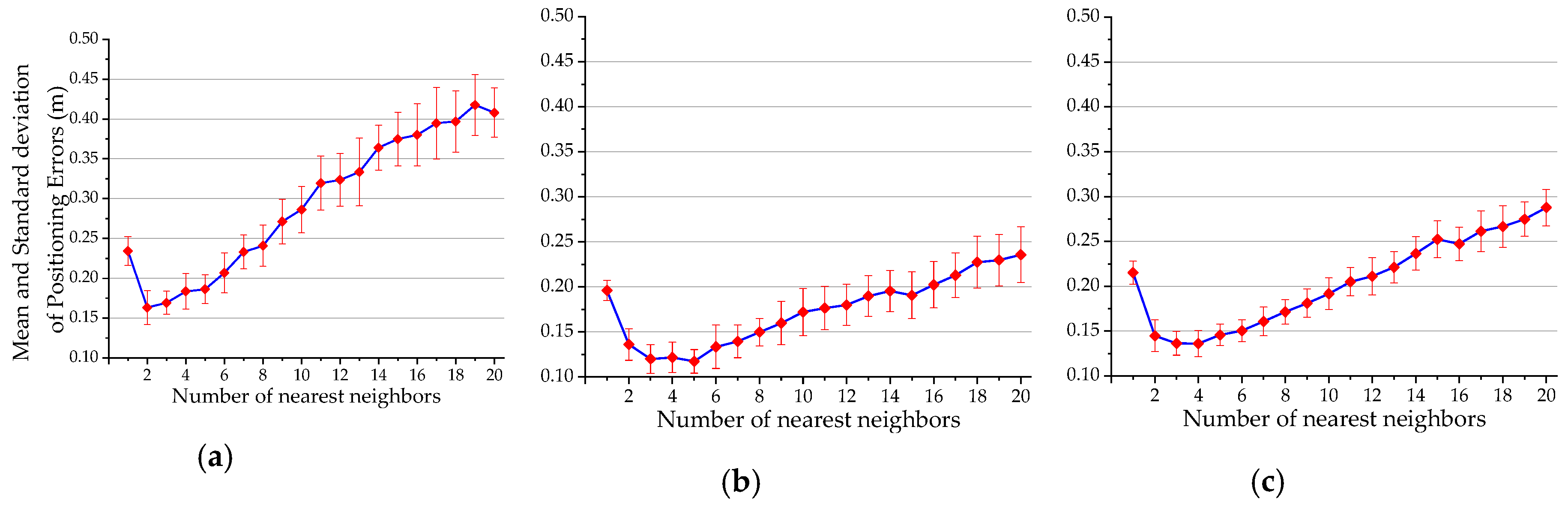
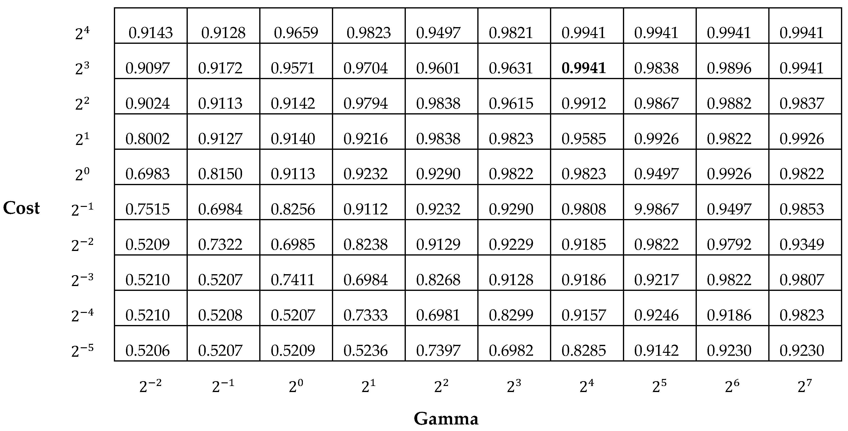
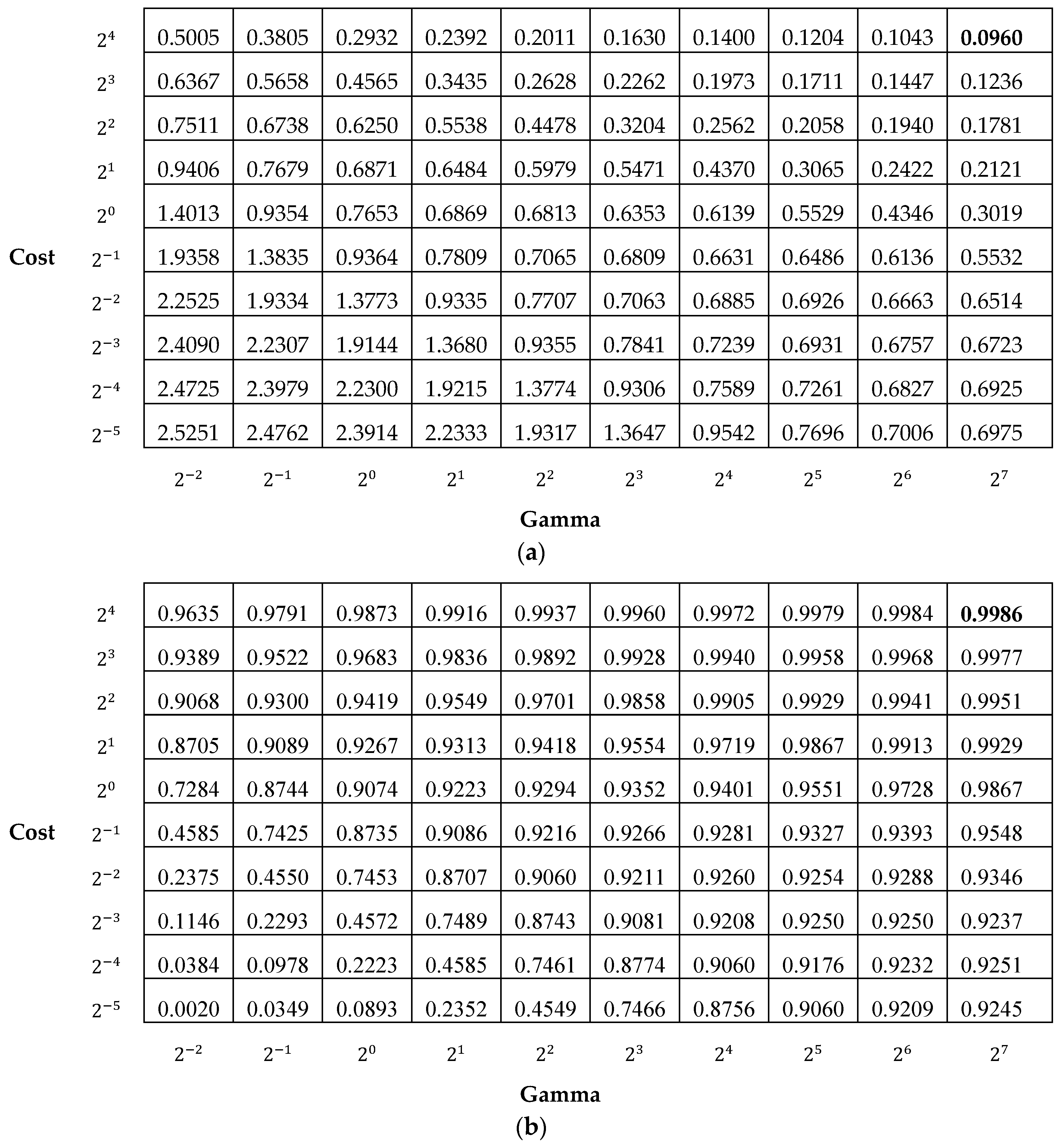
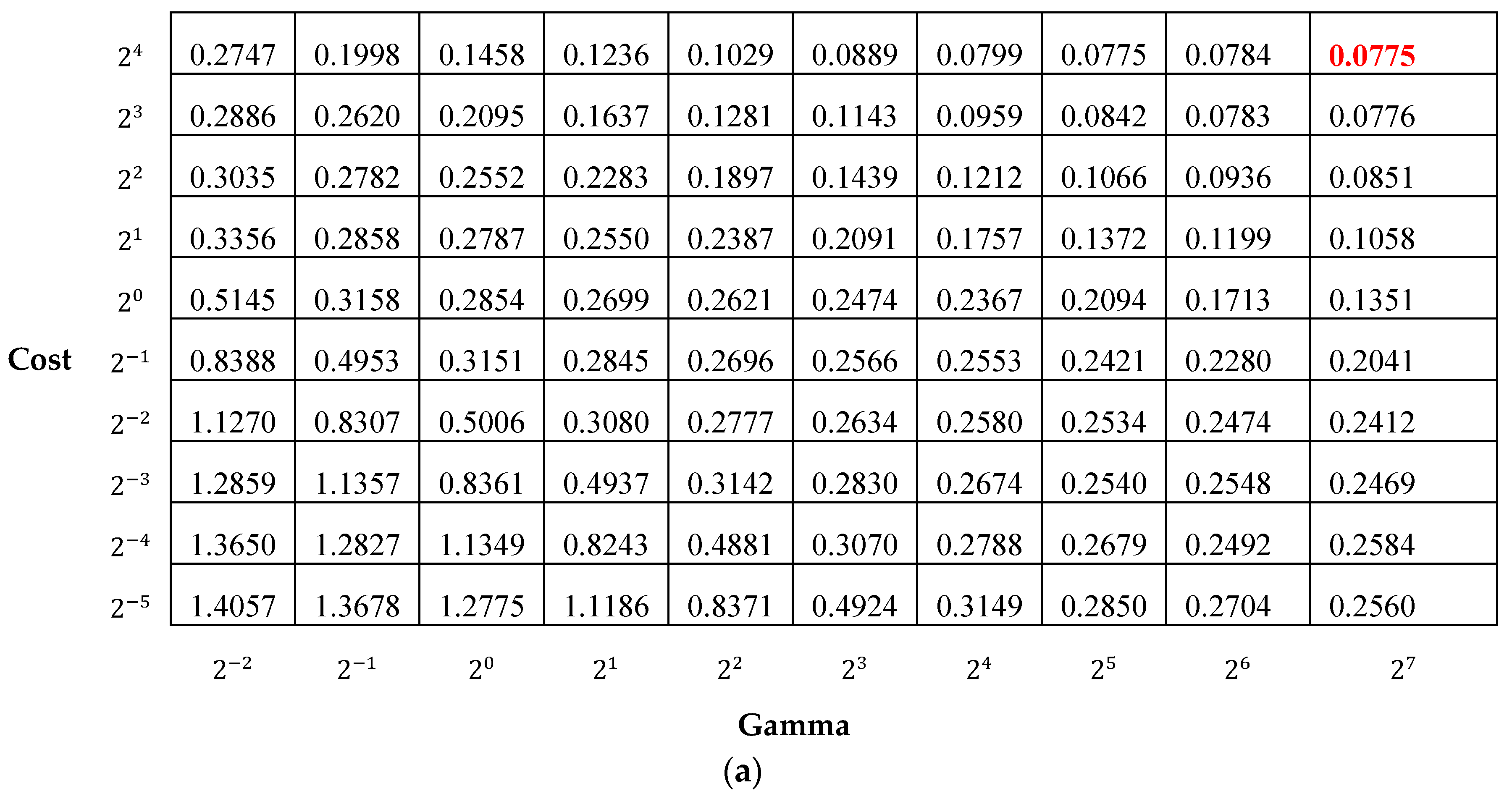
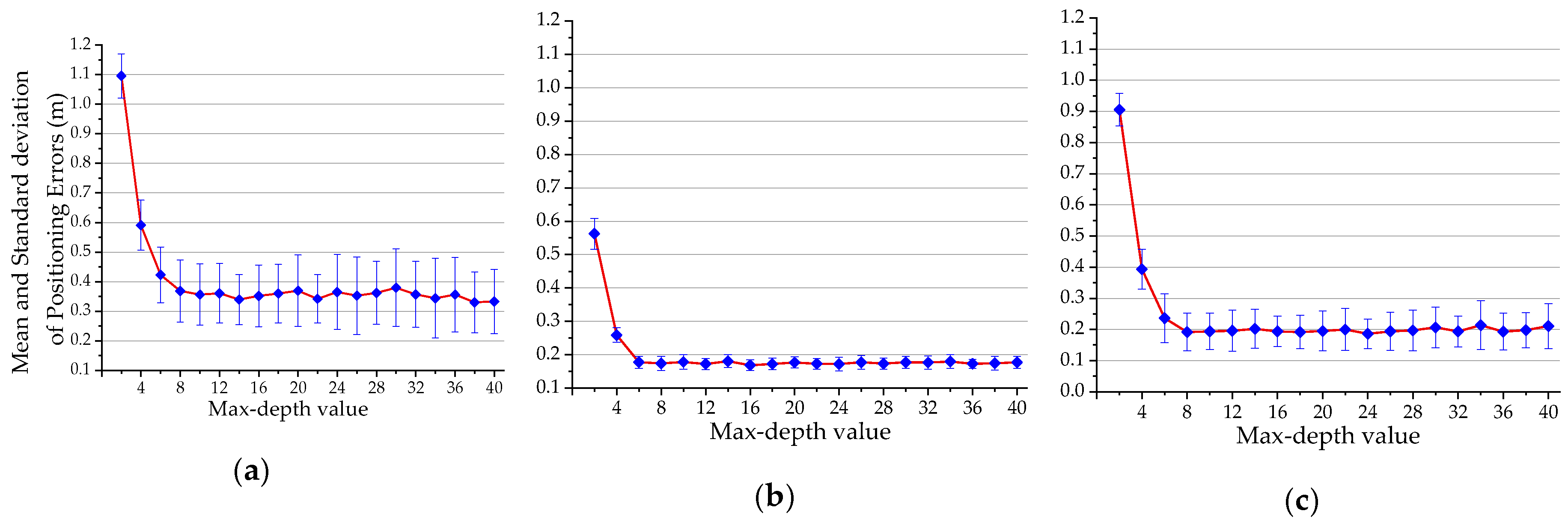
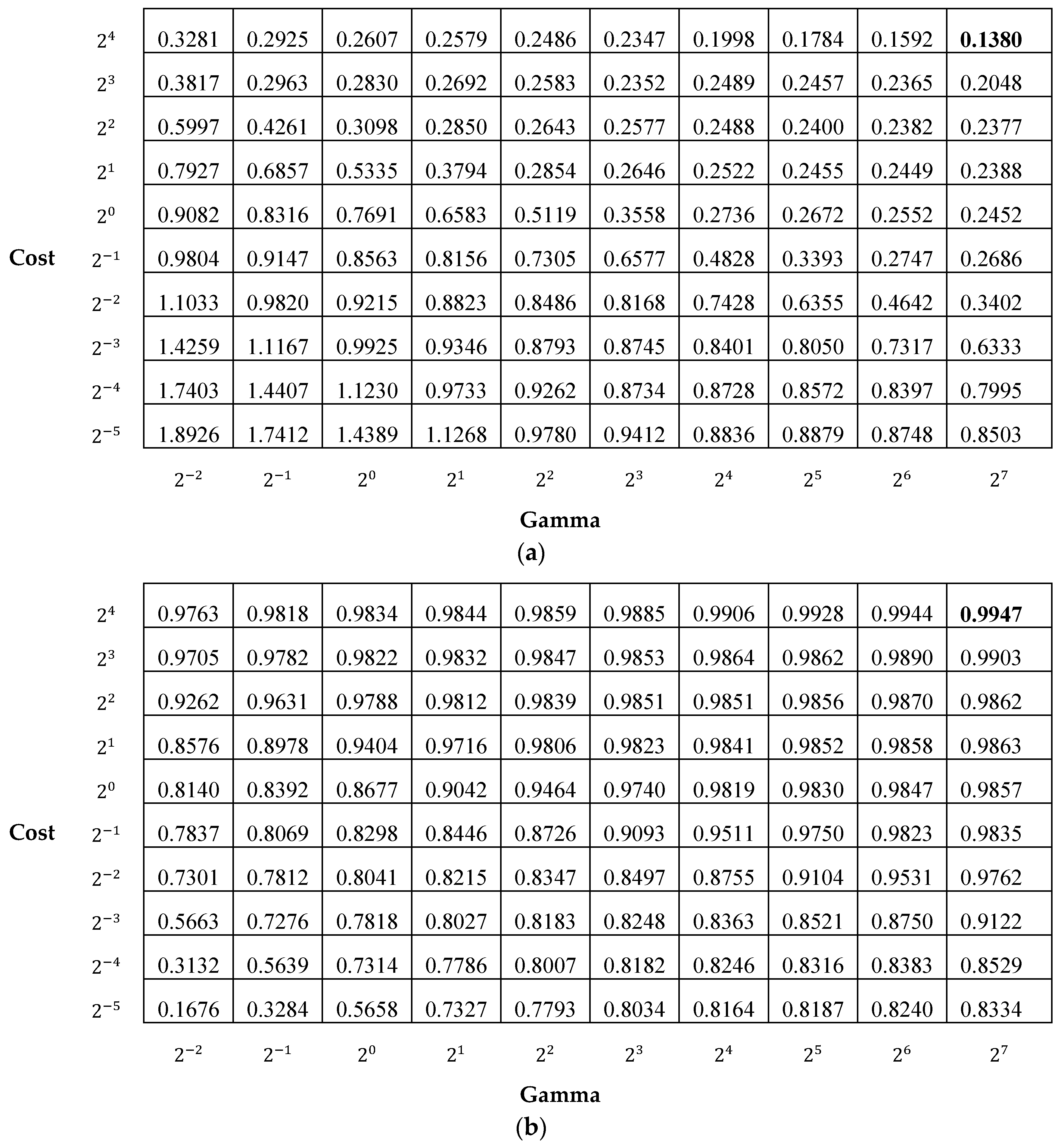
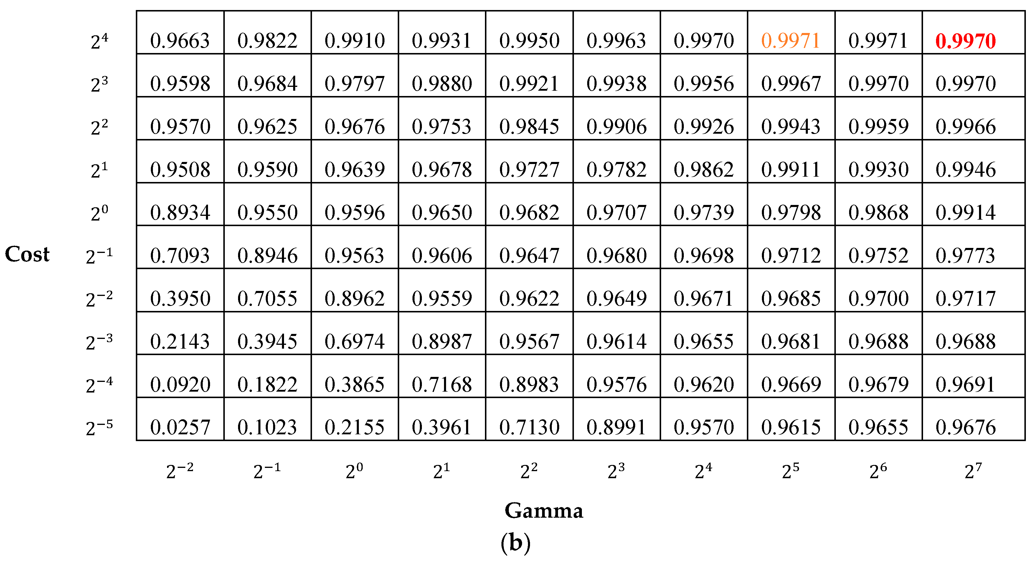
After finishing the noise reduction and area division processes, we estimated the position of the optical receiver as accurately as possible. As mentioned earlier, the ML algorithms used in this article are dual-function, hence SVM, DT, RF, and kNN continue to be adopted with the regression function. From the optimal parameters analysis in the next Section (Table 2), we have the basis to make the final estimation step. This process helps to model a target value based on independent predictors. In this work, the root mean square error (RMSE) was calculated to estimate the skill of the regression predictive model. The results of the location prediction process, as well as the positioning quality comparison of each method, are fully presented and thoroughly explained in Section 5.

4. Tuning Parameters and Results Assessment

Each algorithm has different influential parameters. Optimizing these parameters improves the performance of the algorithms. In this Section, we evaluate algorithm performance by using the CV method and find the optimal parameters for each algorithm [33].

4.1. Algorithms Performance Assessment via K-Fold CV

Two undesirable phenomena that may appear after predicting unseen datasets using ML algorithms are underfitting or overfitting. Underfitting occurs when the model cannot account for the data, and this leads to inaccuracy in the estimated results. Overfitting occurs when there is excellent performance with the available training data, but poor performance with an unknown dataset [34]. To identify these problems, the K-fold CV model evaluation method is a simple and effective approach. In this method, the dataset is divided into K groups and each group is a test set one time, to check and evaluate the performance of the executing algorithm (Figure 10). In this study, K = 10 was used.
C V K F o l d = 1 K j = 1 K M S E j

4.2. Parameter Optimization and Accuracy Assessment

4.2.1. The kNN Algorithm

The kNN algorithm is a non-parametric method based on the idea that k nearest samples to the current sample will be determined, then the Euclidean distance is computed. The chosen k value has a profound impact on the performance of the kNN algorithm [21]. Depending on the specific function (classification or regression), the analysis for selecting the k value has certain differences. However, the simplest way to find the k value is to check the average precision score using different k values. The best overall value of k is chosen, based on the highest precision scores and the highest values of the corresponding CV score. In our case, k was in the range of 2 to 20.
• Classification Function
To optimize the k value for the classification process using the kNN algorithm, the mean of the precision score and CV score was compared for each k value. As depicted in Figure 11, when k increased from 8 to 20, the mean score gradually decreased for both CV and precision. The highest precision score, 0.92, appeared at k = 5. At k = 5, the CV score was 0.96, which ranks second of all the cases. Therefore, we adopted k = 5 as an optimal value for the classification function.
• Regression Function
To maximize the positioning accuracy in the regression process, we conducted a detailed survey of the relationship between the average positioning accuracy, standard deviation, and different k values. In Figure 12a, the best mean of positioning error was obtained when k = 2. However, the standard deviation for k = 2 was worse than that of k = 3, in which the error increased, but not significantly (3.6%). From these considerations, k = 3 was used to estimate the position for the whole floor before area division. Similarly, the same values of k were also selected for the center area and the edge area (see Figure 12b,c)

4.2.2. The SVM Algorithm

SVM is a supervised ML algorithm that can be used to resolve the classification and regression problems, based on a separating hyperplane [34]. In this study, the radial basis function (RBF) kernel was used. Two parameters that need to be optimized for the RBF kernel SVM are Cost and Gamma. When the Cost is small, low bias but high variance may occur, and vice versa. Gamma affects the smoothing of the hyperplane shape [35]. Therefore, optimizing these parameters is a critical procedure. This optimization can be done by the CV method [36]. In this study, a very wide range of Cost values was proposed: from 2 5 to 2 4 . Similarly, the Gamma range was from 2 2 to 2 7 .
• Classification Function
To evaluate the classification ability of SVM, we used the CV technique to assess how accurately this method can perform in practice. The final mean scores corresponding to the values of Cost and Gamma after 10-fold CV are illustrated in Figure 13. The highest mean score appeared when Cost = 2 3 and Gamma = 2 4 . These values were used throughout this study when the area division process with SVM was employed.
• Regression Function
In a process similar to the classification process above, we first searched for the best positioning accuracy according to Gamma and Cost parameters, and then we verified the robustness of the SVM algorithm corresponding to the values found by 10-fold CV. On the whole floor and edge area, the best positioning accuracy occurred when Cost = 2 4 and Gamma = 2 7 (Figure 14 and Figure 15). There was a minor problem occurring in the remaining case (Figure 16), in that the best tuning parameters were not the choice when reassessed by CV. For instant, the best choice in Figure 16b appeared when Gamma = 2 5 and Cost = 2 4 (orange text), while the best value of Gamma and Cost, in Figure 16a, were 2 7 , and 2 4 , respectively (red text). However, in Figure 16b, the mean CV score in both cases: Gamma = 2 5 , Cost = 2 4 (orange text) and Gamma = 2 7 , Cost = 2 4 (red text) are nearly the same. We, therefore choose Gamma = 2 7 and Cost = 2 4 for our work.

4.2.3. The DT Algorithm

DT is one of the most useful and simple ML algorithms for classification and regression [36]. However, irrelevant attributes within the training data can result in overfitting. This problem can be resolved using the CV method [37]. To optimize the accuracy of DT, the maximum depth of the tree (max-depth) needs to be attained. In the next step, we analyzed the optimal values for the two cases of classification and regression. The max-depth values were manually chosen using the precision score and CV score shown in Figure 17 and Figure 18.
• Classification Function
As can be seen in Figure 17, the mean precision score and CV score gradually improve as the max-depth value increases. However, both these scores are nearly stable when max-depth ≥ 8. To avoid time-consuming computer processing, the smallest possible value is chosen. In this case, max-depth = 8 was the best choice.
• Regression Function
In Figure 18a, the mean and standard deviation of the positioning error were inversely proportional to the max-depth of the tree when the max-depth was in the range of 2 to 8. Then the errors remained almost unchanged as we continued to increase the max-depth. As mentioned earlier, higher values of max-depth result in longer execution times. We therefore chose max-depth = 8 for the whole floor. Similarly, we chose max-depth = 6 for the center area (Figure 18b), and max-depth = 8 for the edge area (Figure 18c).

4.2.4. The RF Algorithm

Like the DT algorithm, the RF algorithm is capable of operating under classification and regression functions. RF is made of a bunch of decision trees using a random subset of data [34]. The number of trees is the most important parameter to optimize with RF algorithms [38]. Based on the data shown in Figure 19 and Figure 20, the selected trees for both cases (i.e., classification and regression) are shown in Table 2.

5. Simulation and Results

5.1. Computational Time Comparison

As depicted in 
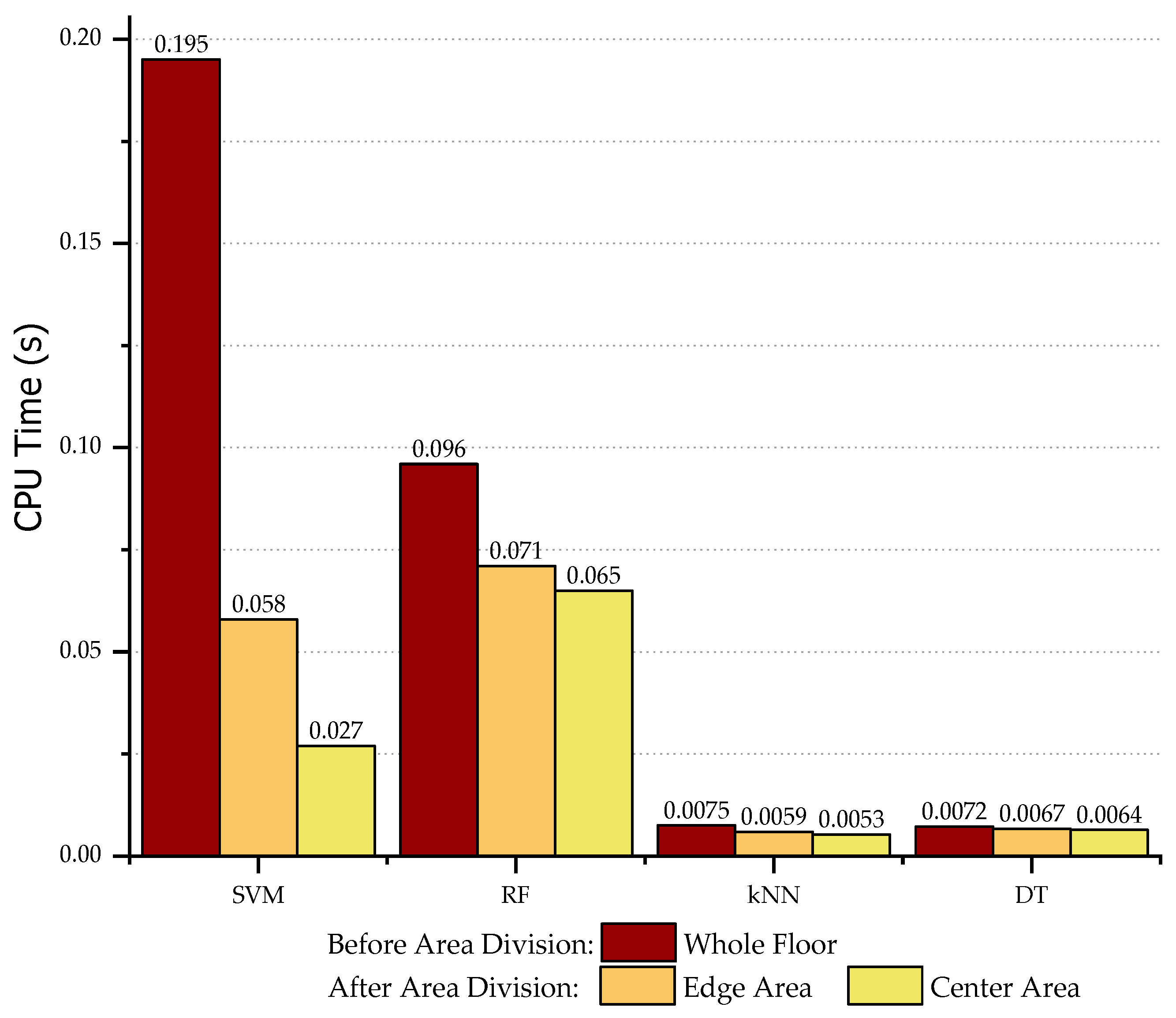
Figure 21, in all four algorithms, there was a significant decrease in the computational time required after applying area division, although each algorithm showed distinct levels of improvement. To compare them with each other, the specific parameters of each algorithm were first optimized. After finding the optimal parameters, the execution time for each method was calculated. The total execution time includes the time spent on the data classification process (for area division) and the location prediction process. In Figure 21, the red column shows the total CPU time before area division, while the orange and yellow columns show the total execution time for unseen data that belong to the edge area and the center area, respectively, after area division. An unknown data can only belong to either the center area or the edge area. Once this data is in the center area, the total CPU time will not include the location estimation time for the edge area data, and vice versa. Table 3 presents the exact time of each method, while the level of improvement in CPU time for each proposed algorithm is shown in Table 4.
It is clear that the system with SVM suffers from the heaviest computation burden but also presents the greatest improvement in execution time after area division. The improvement was 86.21% for the center area and 70.31% for the edge area (see Table 4). The kNN and DT algorithms execute much faster than RF and SVM, with total times of 7.5 ms, and 7.19 ms, respectively. Furthermore, unlike SVM, the time improvement in DT is the lowest of the four suggested methods, with 10.85% for the center area and 6.4% for the edge area. In summary, all four methods show a significant reduction in computation cost after area division is performed using classification.

5.2. Positioning Accuracy Assessment

We performed simulations to evaluate the effectiveness of each algorithm. As shown in 
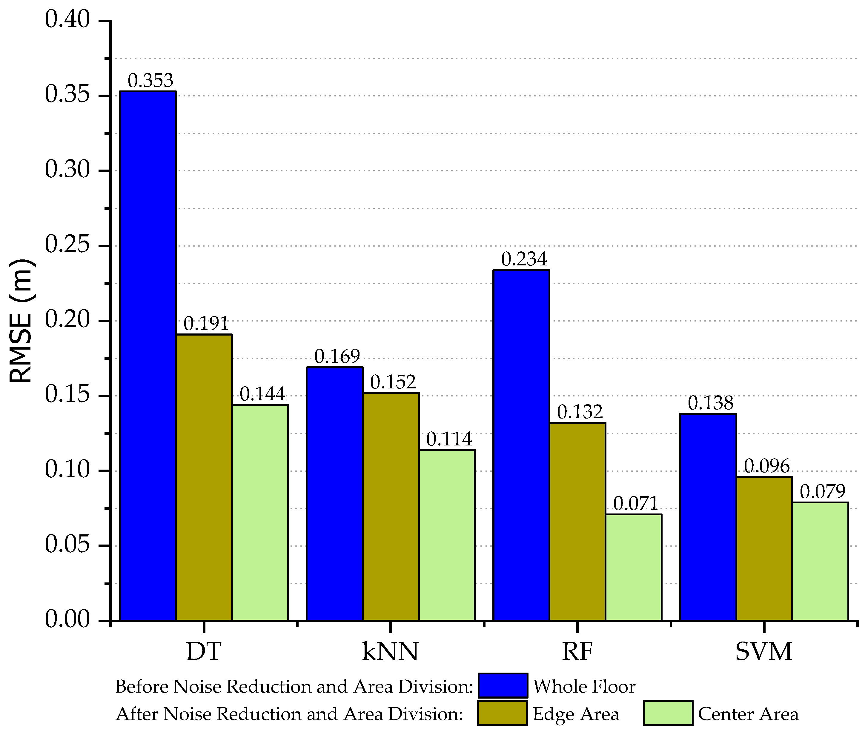
Figure 22, all four methods exhibited a significant decrease in positioning error after noise reduction and area division, although improvement levels varied. As seen in Table 5, DT demonstrated the most positive change, with 59.21% improvement for the center area, and 45.89% improvement for the edge area. The least improved method was kNN, which showed 32.54% improvement and 10.06% improvement for the center area and edge area, respectively. The RF and SVM algorithms also showed a very positive improvement when the average RMSE percentage was approximately the same and around 37%.
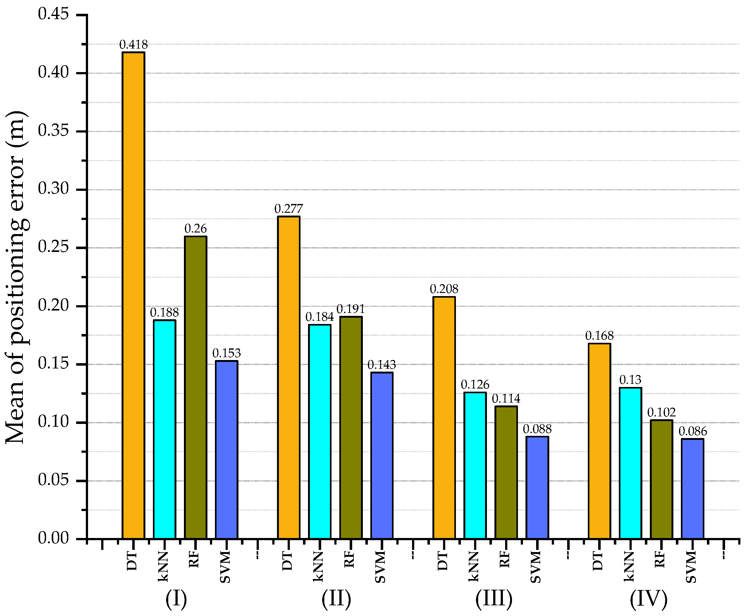
To acquire a more accurate assessment of the degree of influence of each process (i.e., noise reduction and area division) on the final positioning accuracy, the RMSEs of each algorithm (i.e., DT, kNN, RF, and SVM) are surveyed under four cases (Figure 23):
  • (I): Without noise reduction and without area division
  • (II): Without noise reduction and with area division
  • (III): With noise reduction and without area division
  • (IV): With noise reduction and with area division
Case II (incorporating area division) showed a relatively small improvement in the RMSE, with the kNN and SVM algorithms showing 2.13% and 6.54% improvement, respectively. This means that area division has a negligible effect on these two algorithms in term of accuracy. In contrast, the DT and RF algorithms were strongly influenced by the area division process, showing an improvement of 33.73% and 26.54%, respectively.
Case III, with noise reduction and no area division, showed a very promising decline in positioning errors compared to Case I. SVM achieved the best improvement, followed by RF. The DT algorithm continued to show the lowest level of accuracy.
It is clear that the mean positioning errors tended to gradually improve progressing from Case I to Case IV. The highest accuracy (8.6 cm) occurs with SVM in Case IV. The worst accuracy (16.8 cm) occurs with DT. It is interesting to note, however, that the DT algorithm had the highest improvement, showing an RSME reduction of nearly 60% (from 48.1 cm in Case I to 16.8 cm in Case IV). Also, RF showed the same improvement level as DT but RF has a much better positioning accuracy of 10.2 cm. This result is only slightly worse than SVM. Of the four algorithms, kNN shows the least improvement at 30.85%.
In summary, all four methods achieve better positioning accuracy after noise reduction and area division, in the following ascending order of accuracy: DT, kNN, RF, and SVM. The area division technique had a relatively small impact on the accuracy of kNN and SVM, although it did provide significant savings in execution time, as was discussed in the previous Section.
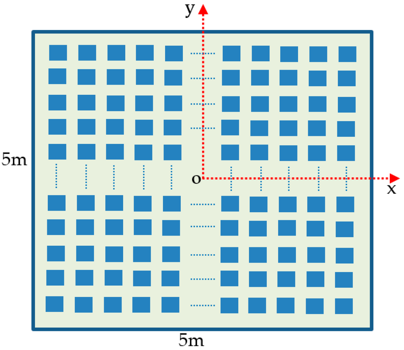
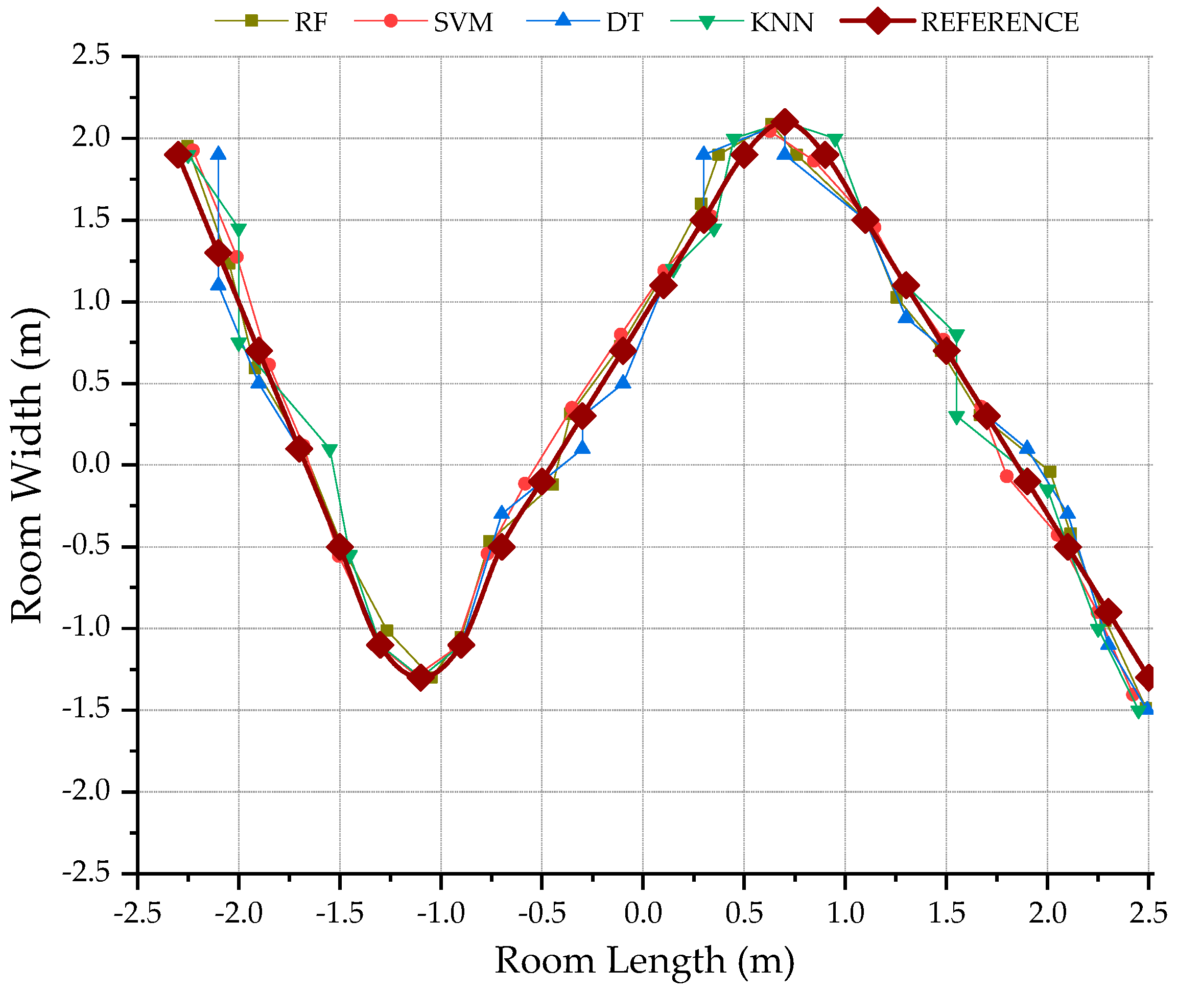
Next, we analyzed the positioning errors, based on the hypothetical roadmap of a mobile robot. On this route, the robot started from the left upper corner, as shown in Figure 24, then went to the opposite position with LED 1 (see Figure 1), then proceeded through the center of the floor and the area near the wall. Finally, the robot went to the corner opposite the start point. Since the effects of multipath reflections and noises varied greatly from location to location in the room, this route helped us to evaluate the efficiency of the proposed solution under varying conditions.
Before applying our proposed solution, the positioning errors in the two corners were very bad (Figure 24). A contrasting image, however, is shown in Figure 25, which shows the results after our solution is deployed. The errors significantly decreased, although the corner area still showed the least accuracy, due to multipath reflections and noises. Furthermore, positioning quality is also better expressed in the remaining areas in which the SVM and RF algorithms provided the best results. Although each method has its own advantages and disadvantages, they all showed a significant improvement in positioning accuracy after applying both area division and noise reduction.

6. Conclusions

In summary, the simulation results showed that after applying the proposed solution, the SVM and RF methods obtained the highest positioning accuracy, at 8.6 cm and 10.2 cm, respectively. The SVM algorithm had the best improvement in execution time (approximately 78%). Our results indicated that if practical applications need a low positioning error, SVM is the optimal option. For applications that need fast execution time but moderate accuracy, we suggest kNN, which demonstrated a positioning accuracy of 13 cm and an average computational time of 5.6 ms.
In this article, we proposed an enhanced ML-based indoor positioning solution using LED lights. Our solution not only improved positioning accuracy, but also reduced computational time. In addition to using signal pre-processing to achieve more accurate positioning, the novel adoption of dual-function ML was employed. The classification function saved execution time and provided a slight improvement in positioning accuracy, while the regression function helped determine the exact location of the object in the final step. In particular, this study compared four popular ML algorithms: SVM, DT, RF, and kNN. The results from this comparison gave us a comprehensive view of the advantages and disadvantages of each algorithm in positioning applications using VLC.
Because developing VLC-based indoor mobile robot applications is our main pursuit, the optimization of ML algorithms to improve positioning accuracy and execution time in a real environment is our highest priority. In our future work, we continue to optimize positioning accuracy using deep machine learning.

Author Contributions

H.Q.T. proposed the idea, designed the proposed algorithm, performed the simulation, and wrote the manuscript. As the corresponding author, C.H. supervised the research, provided the guidance for data analysis, and revised the article.

Acknowledgments

This work was supported by Korea Hydro & Nuclear Power company through the project “Nuclear Innovation Center for Haeoleum Alliance”.

Conflicts of Interest

The authors declare no conflict of interest.

References

  1. Armstrong, J.; Sekercioglu, Y.A.; Neild, A. Visible light positioning: A roadmap for international standardization. IEEE Commun. Mag. 2013, 51, 68–73. [Google Scholar] [CrossRef]
  2. Rajagopal, S.; Roberts, R.D.; Lim, S. IEEE 802.15.7 visible light communication: Modulation schemes and dimming support. IEEE Commun. Mag. 2012, 50, 72–82. [Google Scholar] [CrossRef]
  3. IEEE Draft Standard for Local and Metropolitan Area Networks—Part 15.7: Short-Range Optical Wireless Communications; IEEE P802.15.7/D3; Institute of Electrical and Electronics Engineers (IEEE): Englewood, CO, USA, 1 January 2018; pp. 1–412.
  4. Keskin, M.F.; Sezer, A.D.; Gezici, S. Localization via Visible Light Systems. Proc. IEEE 2018, 106, 1063–1088. [Google Scholar] [CrossRef]
  5. Indoor Positioning: Perfect Light, Precise Location. Available online: http://www.lighting.philips.com/main/systems/lighting-systems/indoor-positioning (accessed on 3 February 2019).
  6. Qiu, K.; Zhang, F.; Liu, M. Let the Light Guide Us: VLC-Based Localization. IEEE Robot. Autom. Mag. 2016, 23, 174–183. [Google Scholar] [CrossRef]
  7. Murai, R.; Sakai, T.; Kawano, H.; Matsukawa, Y.; Kitano, Y.; Honda, Y.; Campbell, K.C. A novel visible light communication system for enhanced control of autonomous delivery robots in a hospital. In Proceedings of the 2012 IEEE/SICE International Symposium on System Integration (SII), Fukuoka, Japan, 16–18 December 2012; pp. 510–516. [Google Scholar] [CrossRef]
  8. Zhuang, Y.; Hua, L.; Qi, L.; Yang, J.; Cao, P.; Cao, Y.; Wu, Y.; Thompson, J.; Haas, H. A Survey of Positioning Systems Using Visible LED Lights. IEEE Commun. Surv. Tutor 2018, 20, 1963–1988. [Google Scholar] [CrossRef]
  9. Do, T.-H.; Yoo, M. An in-Depth Survey of Visible Light Communication Based Positioning Systems. Sensors 2016, 16, 678. [Google Scholar] [CrossRef]
  10. Yang, C.; Shao, H. WiFi-based indoor positioning. IEEE Commun. Mag. 2015, 53, 150–157. [Google Scholar] [CrossRef]
  11. Akram, B.A.; Akbar, A.H.; Shafiq, O. HybLoc: Hybrid Indoor Wi-Fi Localization Using Soft Clustering-Based Random Decision Forest Ensembles. IEEE Access 2018, 6, 38251–38272. [Google Scholar] [CrossRef]
  12. Li, Z.; Braun, T.; Zhao, X.; Zhao, Z.; Hu, F.; Liang, H. A Narrow-Band Indoor Positioning System by Fusing Time and Received Signal Strength via Ensemble Learning. IEEE Access 2018, 6, 9936–9950. [Google Scholar] [CrossRef]
  13. Faragher, R.; Harle, R. Location Fingerprinting with Bluetooth Low Energy Beacons. IEEE J. Sel. Areas Commun. 2015, 33, 2418–2428. [Google Scholar] [CrossRef]
  14. Zou, H.; Wang, H.; Xie, L.; Jia, Q. An RFID indoor positioning system by using weighted path loss and extreme learning machine. In Proceedings of the 2013 IEEE 1st International Conference on Cyber-Physical Systems, Networks, and Applications (CPSNA), Taipei, Taiwan, 19–20 August 2013; pp. 66–71. [Google Scholar] [CrossRef]
  15. Lin, B.; Ghassemlooy, Z.; Lin, C.; Tang, X.; Li, Y.; Zhang, S. An Indoor Visible Light Positioning System Based on Optical Camera Communications. IEEE Photonics Technol. Lett. 2017, 29, 579–582. [Google Scholar] [CrossRef]
  16. Lei, Q.; Zhang, H.; Sun, H.; Tang, L. Fingerprint-Based Device-Free Localization in Changing Environments Using Enhanced Channel Selection and Logistic Regression. IEEE Access 2018, 6, 2569–2577. [Google Scholar] [CrossRef]
  17. Zhang, J.; Xiao, W.; Zhang, S.; Huang, S. Device-Free Localization via an Extreme Learning Machine with Parameterized Geometrical Feature Extraction. Sensors 2017, 17, 879. [Google Scholar] [CrossRef] [PubMed]
  18. Guo, X.; Shao, S.; Ansari, N.; Khreishah, A. Indoor Localization Using Visible Light via Fusion of Multiple Classifiers. IEEE Photonics J. 2017, 9, 1–16. [Google Scholar] [CrossRef]
  19. Yuan, T.; Xu, Y.; Wang, Y.; Han, P.; Chen, J. A Tilt Receiver Correction Method for Visible Light Positioning Using Machine Learning Method. IEEE Photonics J. 2018, 10, 1–12. [Google Scholar] [CrossRef]
  20. Xie, C.; Guan, W.; Wu, Y.; Fang, L.; Cai, Y. The LED-ID Detection and Recognition Method Based on Visible Light Positioning Using Proximity Method. IEEE Photonics J. 2018, 10, 1–16. [Google Scholar] [CrossRef]
  21. Tran, H.Q.; Ha, C. Fingerprint-Based Indoor Positioning System Using Visible Light Communication—A Novel Method for Multipath Reflections. Electronics 2019, 8, 63. [Google Scholar] [CrossRef]
  22. Komine, T.; Nakagawa, M. Fundamental analysis for visible-light communication system using LED lights. IEEE Trans. Consum. Electron. 2004, 50, 100–107. [Google Scholar] [CrossRef]
  23. Gfeller, F.R.; Bapst, U. Wireless in-house data commin detaiunication via diffuse infrared radiation. Proc. IEEE 1979, 67, 1474–1486. [Google Scholar] [CrossRef]
  24. Sadowski, S.; Spachos, P. RSSI-Based Indoor Localization with the Internet of Things. IEEE Access 2018, 6, 30149–30161. [Google Scholar] [CrossRef]
  25. Ghassemlooy, Z.; Popoola, W.; Rajbhandari, S. Optical Wireless Communications, System and Channel Modeling with MATLAB; CRC Press: Boca Raton, FL, USA, 2012; ISBN 9781439851883. [Google Scholar]
  26. Mohammed, N.; Elkarim, M. Exploring the effect of diffuse reflection on indoor localization systems based on RSSI-VLC. Opt. Express 2015, 23, 20297–20313. Available online: https://www.osapublishing.org/oe/abstract.cfm?uri=oe-23-16-20297 (accessed on 22 February 2019). [CrossRef] [PubMed]
  27. Lu, X.; Zou, H.; Zhou, H.; Xie, L.; Huang, G. Robust Extreme Learning Machine With its Application to Indoor Positioning. IEEE Trans. Cybern. 2016, 46, 194–205. [Google Scholar] [CrossRef] [PubMed]
  28. Gu, W.; Aminikashani, M.; Deng, P.; Kavehrad, M. Impact of Multipath Reflections on the Performance of Indoor Visible Light Positioning Systems. J. Lightw. Technol. 2016, 34, 2578–2587. [Google Scholar] [CrossRef]
  29. Boucouvalas, A.C. Indoor ambient light noise and its effect on wireless optical links. IEE Proc. J. Optoelectron. 1996, 143, 334–338. [Google Scholar] [CrossRef]
  30. Downey, A.B. Think DSP—Digital Signal Processing in Python; O’Reilly: Sebastopol, CA, USA, 2016; ISBN 978-1-491-93845-4. [Google Scholar]
  31. Tagare, P. Signal averaging. In Biomedical Digital Signal Processing; Tompkins, W.J., Ed.; Prentice-Hall, Inc.: Upper Saddle River, NJ, USA, 1993; pp. 184–192. [Google Scholar]
  32. Alin, C.; Barthélemy, C.; Luc, C.; Valentin, P.; Mihai, D. Evaluation of the noise effects on visible light communications using Manchester and Miller coding. In Proceedings of the 2014 International Conference on Development and Application Systems (DAS), Suceava, Romania, 15–17 May 2014; pp. 85–89. [Google Scholar]
  33. Pedregosa, F.; Varoquaux, G.; Gramfort, A.; Michel, V.; Thirion, B.; Grisel, O.; Blondel, M.; Prettenhofer, P.; Weiss, R.; Vanderplas, J.; et al. Scikit-learn: Machine Learning in Python. J. Mach. Learn. Res. 2011, 12, 2825–2830. [Google Scholar]
  34. Friedman, J.; Hastie, T.; Tibshirani, R. The Elements of Statistical Learning. In Data Mining, Inference and Prediction; Springer: New York, NY, USA, 2008; ISBN 978-0387848570. [Google Scholar]
  35. Ben-Hur, A.; Weston, J. A User’s Guide to Support Vector Machines. Data Mining Techniques for the Life Sciences; Springer: New York, NY, USA, 2010; pp. 223–239. [Google Scholar] [CrossRef]
  36. James, G.; Witten, D.; Hastie, T.; Tibshirani, R. An Introduction to Statistical Learning with Application in R; Springer: New York, NY, USA, 2014; ISBN 978-1461471370. [Google Scholar]
  37. Bramer, M. Avoiding Overfitting of Decision Trees. In Principles of Data Mining. Undergraduate Topics in Computer Science; Springer: London, UK, 2013. [Google Scholar] [CrossRef]
  38. Breiman, L. Random Forests. Mach. Learn. 2001, 45, 5. [Google Scholar] [CrossRef]
Figure 1. Typical room and channel model.
Applsci 09 01048 g001
Figure 2. Fingerprints on the floor.
Applsci 09 01048 g002
Figure 3. Design of prototype. (a) On-Off keying (OOK) modulation using Manchester encoding. (b) Time-division multiplexing (TDM) protocol.
Applsci 09 01048 g003
Figure 4. Signal-To-Noise Ratio (SNR) by: (a) line-of-sight (LOS) channel, (b) diffuse channel, and (c) overall channel.
Applsci 09 01048 g004
Figure 5. Positioning error using a Trilateration algorithm: (a) without multipath reflections and (b) with multipath reflections.
Applsci 09 01048 g005
Figure 6. Proposed study method.
Applsci 09 01048 g006
Figure 7. Sampling data by: (a) LOS signals and (b) diffuse signals.
Applsci 09 01048 g007
Figure 8. Mean received optical power with different reflection rates by (a) 0.2, (b) 0.5, and (c) 0.8.
Applsci 09 01048 g008
Figure 9. Received optical power with different reflection rates by (a) 0.2, (b) 0.5, and (c) 0.8.
Applsci 09 01048 g009
Figure 10. K-Fold Cross-Validation (CV).
Applsci 09 01048 g010
Figure 11. Mean score vs. number of nearest neighbors.
Applsci 09 01048 g011
Figure 12. The mean and standard deviation of positioning errors vs. number of nearest neighbors by: (a) whole floor, (b) center area, and (c) edge area.
Applsci 09 01048 g012
Figure 13. Mean score after CV.
Applsci 09 01048 g013
Figure 14. The mean score in the whole area of: (a) positioning accuracy and (b) CV.
Applsci 09 01048 g014
Figure 15. The mean score in the edge area of: (a) positioning accuracy and (b) CV.
Applsci 09 01048 g015
Figure 16. The mean score in the center area of: (a) positioning accuracy and (b) CV.
Applsci 09 01048 g016aApplsci 09 01048 g016b
Figure 17. Mean score vs. max-depth.
Applsci 09 01048 g017
Figure 18. Mean and standard deviation of positioning errors vs. max-depth by: (a) whole floor, (b) center area, and (c) edge area.
Applsci 09 01048 g018
Figure 19. Mean score vs. number of trees.
Applsci 09 01048 g019
Figure 20. Mean and standard deviation of positioning errors vs. number of trees by: (a) whole floor, (b) center area, and (c) edge area.
Applsci 09 01048 g020
Figure 21. Computational time comparison before and after area division.
Applsci 09 01048 g021
Figure 22. RMSE comparison.
Applsci 09 01048 g022
Figure 23. Detailed mean of positioning error comparison.
Applsci 09 01048 g023
Figure 24. Estimated route before noise reduction and area division.
Applsci 09 01048 g024
Figure 25. Estimated route after noise reduction and area division.
Applsci 09 01048 g025
Table 1. Visible Light Communication (VLC) parameters.
ObjectParameterValue
Simulation spaceRoom dimension (Length × Width × Height)5 m × 5 m × 2.5 m
Reflective rate0.8
Optical transmitterLED power25 W
Number of LED bulbs4
LED bandwidth3 MHz
Data rate2 Mbps
LED position (x, y, z) (m)LED 1 (−1.25, −1.25, 2.5)
LED 2 (1.25, −1.25, 2.5)
LED 3 (1.25, 1.25, 2.5)
LED 4 (−1.25, 1.25, 2.5)
Half power semi-angle70°
Optical receiverPD active area1 cm2
Field-of-view70°
Sensitivity−30 dBm
Gain of optical filter1
Refractive index of optical concentrator1.5
PD responsivity0.54 A/W
Table 2. Optimal parameters.
Algorithm (Optimized Parameter)ClassificationRegression
Whole FloorCenter AreaEdge Area
kNN (k)5333
SVM (Gamma and C)16 and 8128 and 16128 and 16128 and 16
DT (Max-depth)8868
RF (Tree)16121612
Table 3. Computational time (ms).
AlgorithmsPosition of DataArea Division TimeLocation Prediction TimeTOTAL TIME
SVMWhole floorNo classification195.00195.00
Center Area6.9020.0026.90
Edge Area6.9051.0057.90
RFWhole floorNo classification96.0096.00
Center Area11.0054.0065.00
Edge Area11.0060.0071.00
kNNWhole floorNo classification7.507.50
Center Area0.594.705.29
Edge Area0.595.305.89
DTWhole floorNo classification7.197.19
Center Area1.105.316.41
Edge Area1.105.636.73
Table 4. CPU time level of improvement after area division (%).
Position of DataSVMRFkNNDT
Center86.21 32.2929.4710.85
Edge70.3126.0421.476.40
Average78.2629.1725.479.63
Table 5. Root mean square error (RMSE) comparison (%).
Position of DataDTkNNRFSVM
Center59.2132.5446.1842.75
Edge45.8910.0628.9030.43
Average52.5521.3037.5436.59

