WAMS-Based Online Disturbance Estimation in Interconnected Power Systems Using Disturbance Observer

Abstract

In the event of a generator loss or disturbance, the power system frequency declines quickly and overall system stability is at risk. During these scenarios, under frequency load shedding is triggered to restore the power system frequency. The main stage of modern adaptive under frequency load shedding techniques is disturbance estimation. However, the swing equation is widely used in disturbance estimation but has some critical estimation errors. In this paper, instead of using the swing equation we proposed the use of a disturbance observer to estimate the curtailed power. By making use of wide area measurements, a system frequency response model, which is a representative of the whole power system, can be realized in real time. Using different power system states of the developed model, a disturbance observer can be designed as well. The main advantage of the disturbance observer is that it can accurately estimate the disturbance magnitude and its location in a very short time. Further investigations show that by using the disturbance observer disturbances, which occur at the same time or at different times in different areas regardless of the magnitude or size, accurate estimations can be made. To ascertain the efficiency of the proposed scheme, simulations are done for a four-area power system using Matlab/Simulink.

1. Introduction

With the growth in energy demand and the restructuring of power systems, frequency stability remains an area requiring consistent research. There are many phenomenon that lead to frequency instabilities but all eventually lead to transmission line tripping or generation loss. This upsets the balance between generation and demand and the frequency of a system deviates from the nominal [1,2,3,4]. A scenario where the demand is higher than the generation leads to severe decline in frequency and this is of critical concern for modern power systems.

In such cases, advanced frequency restoration techniques with a high speed of response are required. Under frequency load shedding (UFLS) techniques have been used to restore the power system frequency in the event of a large disturbance. Traditional UFLS technique is the most common and in this scheme specific portions of load are shed instantly whenever a frequency threshold is violated [5,6,7,8,9,10,11,12,13]. This technique only relies on local frequency measurements and the magnitude of the disturbance is not estimated. As a result, the major shortfall of this technique is that it fails to achieve optimum load shedding and it results in either over shedding or under shedding, which further puts the system at risk.

However, it is important that the disturbance amount be accurately estimated in order to maintain system stability. In this regard, adaptive techniques became more preferred to traditional ones [14,15,16,17,18,19,20,21,22]. Adaptive techniques make use of the swing equation to estimate the disturbance. In [15], the magnitude of the disturbance is estimated using the swing equation after which the most optimum amount to be shed is determined. In [16], the aim was to maximize the use of primary frequency support; here UFLS was implemented by taking into account the voltage variations. In [17], based on the estimated power system inertia the disturbance amount is constantly updated after each load shedding stage. In order to achieve the least amount of load shed after obtaining the disturbance amount using the swing equation, the governor ramp shape is then considered in [18]. Nearly similar to the work in [15], in [14] the amount of power deficit is determined using the swing equation and an optimization algorithm is used to determine the optimum amount of load to be shed at each stage.

It can be concluded that disturbance estimation forms the backbone of adaptive stability restoration schemes. It is therefore critical that for any power system the disturbance be correctly estimated. Even though the swing equation is commonly used, it may fail to accurately estimate the disturbance amount. In [23], it was found out that the estimated disturbances differ from the actual occurred disturbance. It is noted that the direction of frequency drift determines whether the estimated disturbance will be large or small. The authors conclude that the error is within a range of $\pm 2.5\%$. However, further investigations show that if the power system modeling is done using highly detailed equations and not just the system frequency response (SFR) model, the estimation error can be way larger. The main reasons for the errors in estimation are the unavailability of accurate power system information and the frequency variations during disturbance.

In such cases where accurate information about the power system state is required, Wide Area Monitoring Systems (WAMS) can be an essential tool in power system dynamic studies [24,25,26]. Since practical electrical grids cover large geographical areas, without the use of WAMS, it was difficult to quickly pick the root cause of system collapse. The extensive use of wide-area measurement systems (WAMS) has brought flexibility in power networks monitoring [27,28,29]. With WAMS event monitoring, control and effects mitigation can now be performed more rapidly [30]. This is because most PMUs are capable of producing 60 samples per second and modern PMUs can produce twice as many samples per second [31]. This sampling rate can guarantee even further reduction in the estimation error.

Another important point to note is that the rate of frequency swing is smaller in the normal operation than when a disturbance occurs. Modern power systems have a large number of renewable energy generation power plants. This affects the overall inertia of the system since power electronic interfaced devices are known to have very low inertia. Both the disturbance and inertia estimation are done using the swing equation. In disturbance estimation, the inertia is assumed a constant and this results in errors. Therefore, it is better to use the dynamics of the whole system rather than just the swing equation to estimate the disturbance. By making use of wide area measurements, an SFR model that accounts for the dynamics of the power system can be realized online. An observer, which replicates the system, can then be designed to estimate the disturbance. The use of observers is commonly applied to direct load frequency control (LFC), for example in [32]. However, we propose the use of the disturbance observer for systems subjected to severe disturbances.

In this paper, we propose two concepts to enhance disturbance estimation. Firstly, instead of only using the swing equation or simply the frequency, different system states are used in the estimation. Based on the developed system frequency response model the equations, which describe the dynamics of the system, are first derived. Using the derived equations, the system matrix, input matrix and the disturbance matrix of the system are developed. Taking into consideration that not all the system states are directly accessible, a state observer is also developed to estimate the unknown states. After which a robust disturbance observer is designed to accurately estimate the disturbance magnitude. In addition to the disturbance estimation, it is shown in the simulations that the disturbance observer can also estimate different sized disturbances, which occurred in different areas. In our simulations a four area interconnected power system is considered. The disturbance observer is designed such that it can estimate a disturbance as well as its location area. Multiple disturbances occurring in different areas can also be measured accurately. With the use of the disturbance observer, the estimation error can be effectively zeroed.

This paper is organized as follows: In Section 2 power system modelling is presented. Section 3 describes the design of the robust disturbance observer and the considered test system is presented in Section 4. Simulations and results are discussed in Section 5. This paper concludes with Section 6 where the advantages and disadvantages of using the disturbance observer are outlined. Furthermore, intended future works are also presented in the last section.

2. WAMS-Based Power System Modeling

2.1. WAMS Model Setup

The use of wide area measurements from phasor measurement units (PMUs) provides new capabilities for more accurate and real time monitoring of power systems [33]. PMUs provide voltage and current phasors as well as frequency and its rate of change, which are useful in power system dynamic studies. Due to their high sampling rates, the online estimation errors are significantly reduced. In [34], a technique that makes use of wide-area frequency measurements is presented for contingency magnitude detection and localization. The given reference shows that by taking advantage of the PMUs data, one can easily express the dynamics for a power system of any size. The use of PMUs reduces the mathematical complexities encountered in fundamental analysis of power system dynamics. Considering the power system dynamics as well as the swing equation, we can come up with the following generalized differential equation

$$\frac{d{x}_i}{dt}=f_i\left(x_i,I_{di},I_{qi},V_i\right)$$

(1)

The various parameters can be further analyzed using the below equations

$$\begin{array}{c}{I}_{di}=h_{di}\left(x_i,V_i,{\theta }_i\right)\hfill \\ I_{qi}=h_{di}\left(x_i,V_i,{\theta }_i\right)\hfill \\ \left(P_{mi}+j{Q}_{mi}\right)+\left(P_{Li}+j{Q}_{Li}\right)=\sum V_i{V}_j{Y}_{ik}{e}^{j\left({\theta }_i-{\theta }_j-{\sigma }_{ik}\right)}\hfill \end{array}$$

(2)

where $P_i,Q_i,V_i,I,\mathrm{and}{\theta }_i$ are the active power, reactive power, bus voltage, currents and electrical angles, respectively. $d,q,L,m$, and i are notations for d-axis, q-axis, loads, generation, and ith busbar, respectively.

Where the state space representation of the above equation can be given as

$$\begin{array}{c}\dot{x}=p\left(x,y,u\right)\hfill \\ 0=q\left(x,y,u\right)\hfill \end{array}$$

(3)

where $x_i,y_i$, and $u_i$ are the state, output, and input vectors, respectively.

From (3), it can be seen that p and q are some known functions. The general assumption which will be consistent in this paper is that the initial values of the system are provided by WAMS. Once the power system operator has the real time information and measurements provided by WAMS platform, the dynamic behavior can be monitored and assessed online.

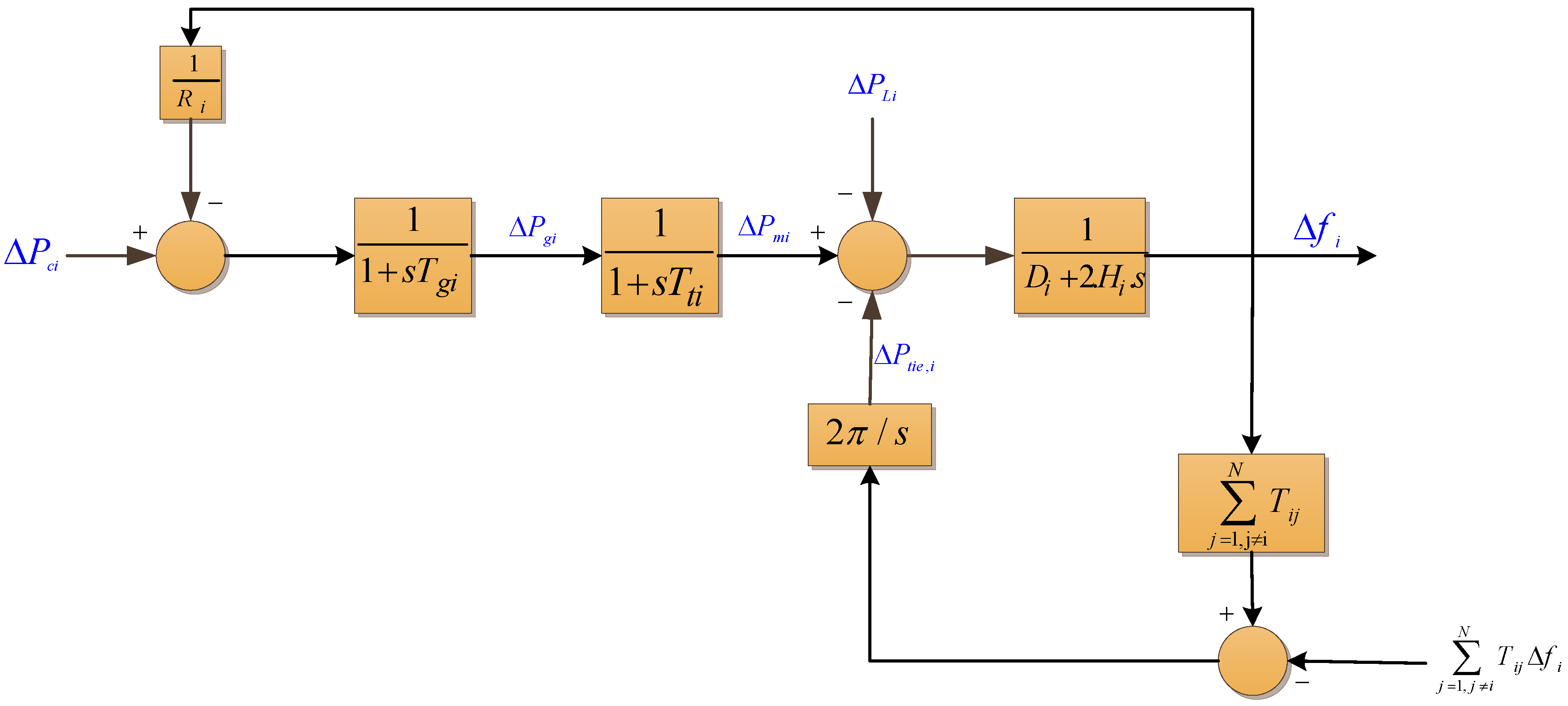
2.2. Power System Dynamic Modelling

The system frequency response (SFR) model has been commonly used to represent the frequency dynamics of a power system [35,36]. The model can make use of re-heated turbines or non-reheated turbines. An SFR model block diagram of a non-reheated power system is shown in Figure 1. Generally, the model is commonly used in load frequency control (LFC) [37,38]. The dynamics of area i considering a multi-area power system is described by the differential Equations (4)–(8). This model can be used for practical power systems modelling and still giving technically sound results.

$$\Delta {\dot{f}}_i=\frac{1}{2H_i}\Delta P_{mi}-\frac{1}{2H_i}\Delta P_{Li}-\frac{D}{2H_i}\Delta f_i-\frac{1}{2H_i}\Delta P_{tie,i}$$

(4)

$$\Delta {\dot{P}}_{mi}=\frac{1}{T_{ti}}\Delta P_{gi}-\frac{1}{T_{ti}}\Delta P_{mi}$$

(5)

$$\Delta {\dot{P}}_{gi}=\frac{1}{T_{gi}}\Delta P_{ci}-\frac{1}{R_i{T}_{gi}}\Delta f_i-\frac{1}{T_{gi}}\Delta P_{gi}$$

(6)

$$\Delta P_{tie,i}=2\pi \sum _{j=1,j\ne i}^N{T}_{ij}\left(\Delta f_i-\Delta f_j\right)$$

(7)

$$\Delta P_{tie,i}=\sum _{i=1}^m\left(\Delta P_{tie,actua{l}_j}-\Delta P_{tie,schedule{d}_j}\right)$$

(8)

where $H_i$ is the inertia, D is the damping coefficient, $T_{ti}$ is the turbine time constant, $T_{gi}$ is the governor time constant, $T_{ij}$ is the tie line coefficient and $R_i$ is the droop. In addition, $\Delta f_i$ is the frequency deviation, $\Delta P_{mi}$ is the mechanical power deviation, $\Delta P_{gi}$ is the governor deviation, $\Delta P_{tie,i}$ is the tie line power deviation and $\Delta P_{ci}$ is the control input.

The overall power system dynamics can be expressed in state space form as follows:

$${\dot{x}}_i=A_i{x}_i\left(t\right)+B_i{u}_i\left(t\right)+F_i\Delta P_i;i=1,2,3\cdots n$$

(9)

where $A_i$, $B_i$, $F_i$, $\Delta P_i$, $x_i$ and $u_i$ are the system matrix, input matrix, disturbance matrix, disturbance, state vector and the input respectively.

2.3. Single Area Dynamics

To implement localized or decentralized disturbance estimation, where each area is responsible for estimating its own disturbance, we consider a single area. Using Equation (9) we can construct matrices that define the dynamics of area i. Firstly, we include the tie line dynamics and the state vector can be described as follows

$$x_i\left(t\right)={\left[\begin{array}{cccc}\Delta f_i& \Delta P_{mi}& \Delta P_{gi}& \Delta P_{tie,i}\end{array}\right]}^T$$

(10)

$$u_i\left(t\right)=\Delta P_{ci}$$

(11)

The matrices with tie line dynamic considered are given in Appendix A. If we neglect the tie line dynamics, we remain with three states as follows:

$$x_i\left(t\right)=\left[\begin{array}{ccc}\Delta f_i& \Delta P_{mi}& \Delta P_{gi}\end{array}\right]$$

(12)

The system matrices then reduce and are given in Appendix A.

2.4. Multi Area Dynamics

In addition to the single area dynamics, we can also consider the multi area dynamics. In real power systems, a single area can represent a power station or a specific region of a large power system. These power stations or regions are then connected together to form an interconnected grid. The control center monitors the whole grid and gives specific commands in emergency scenarios and this is known as centralized disturbance estimation. The general equation for the whole power system becomes

$$\dot{x}\left(t\right)=Ax\left(t\right)+Bu\left(t\right)+F\Delta P$$

(13)

where

$$x\left(t\right)={\left[\begin{array}{ccccc}{x}_1\left(t\right)& x_2\left(t\right)& x_3\left(t\right)& \cdots & x_n\left(t\right)\end{array}\right]}^T$$

(14)

$$u\left(t\right)={\left[\begin{array}{ccccc}{u}_1\left(t\right)& u_2\left(t\right)& u_3\left(t\right)& \cdots & u_n\left(t\right)\end{array}\right]}^T$$

(15)

$$\Delta P={\left[\begin{array}{ccccc}\Delta P_1& \Delta P_2& \Delta P_3& \cdots & \Delta P_n\end{array}\right]}^T$$

(16)

If we neglect the tie line dynamics, for an n area power system the overall matrices are given in the Appendix A. The matrices with tie lines neglected have the following dimension: $A\in {\mathbb{R}}^{3n\times 3n}$, $B\in {\mathbb{R}}^{3n\times 3}$ and $F\in {\mathbb{R}}^{3n\times 3}$. The entire elements are real numbers. If we consider the tie line dynamics, we have $A\in {\mathbb{R}}^{4n\times 4n}$, $B\in {\mathbb{R}}^{4n\times 4}$ and $F\in {\mathbb{R}}^{4n\times 4}$.

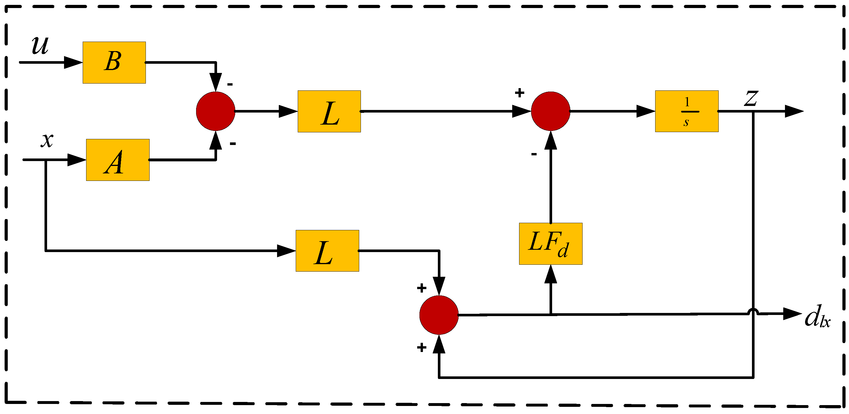
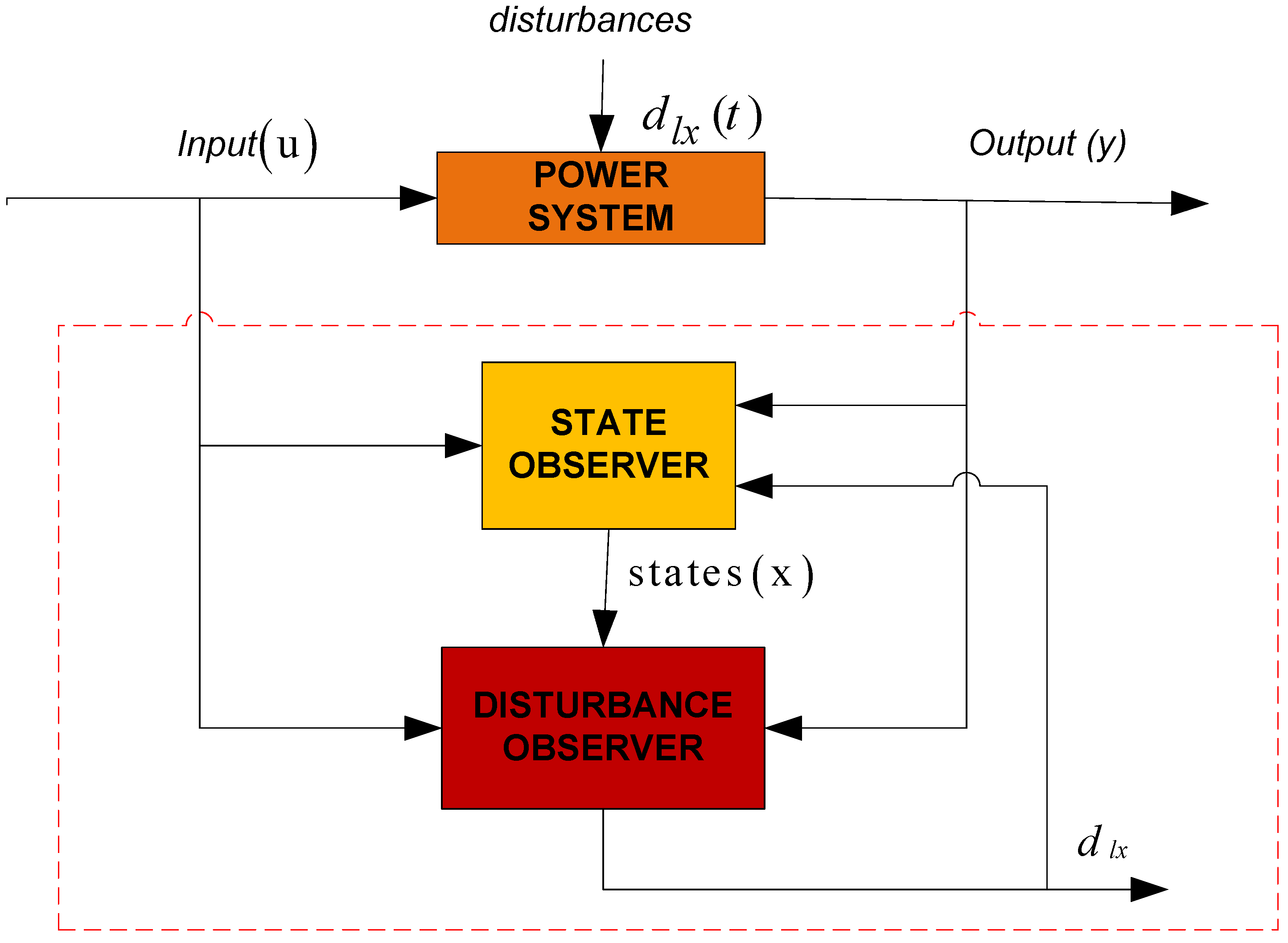
3. Proposed Disturbance Observer-Based Disturbance Estimation

The disturbance observer can be used to accurately estimate the disturbance magnitude. Figure 2 shows the structure of the proposed set up for disturbance estimation. For a disturbance which occurs at any time (t) in a power system. The input and the states of the system obtained via a state observer are required to estimate the disturbance magnitude. The design of both the power system state observer and the disturbance observer are described in what follows.

3.1. State Observer Design

In order to design the disturbance observer we first need to design the state observer to estimate the unknown system states. In real systems, some states might not be directly accessible, hence the need to design a state observer. In control and design, any virtual system driven by the inputs and outputs of the actual system can act as an observer. If we consider a linear time invariant (LTI) system given as

$$\left\{\begin{array}{c}\dot{x}=Ax+Bu+F_d{d}_{lx}\hfill \\ y=Cx+D_{u}u+D_d{d}_y\hfill \end{array}\right.$$

(17)

In a more compact term by taking into account the time varying parameters, the system can be represented as

$$\left\{\begin{array}{c}\dot{x}\left(t\right)=Ax\left(t\right)+Bu\left(t\right)+F_d{d}_{lx}\hfill \\ y\left(t\right)=Cx\left(t\right)\hfill \end{array}\right.$$

(18)

where $D_u=D_d=0$, C is the output matrix.

In state observer design $x\left(t_0\right)=x_0$ is unknown, however, the output variables $y\left(t\right)$ of the original systems are present at any time. This output information is necessary to design a virtual system of the same order, which replicates the dynamics of the original system. From design and experiments, the matrices A, B, $F_d$ and C are known, therefore, the observer can have the following structure

$$\left\{\begin{array}{c}\dot{\widehat{x}}\left(t\right)=A\widehat{x}\left(t\right)+Bu\left(t\right)+F_d\widehat{d_{lx}}\hfill \\ \widehat{y}\left(t\right)=C\widehat{x}\left(t\right)\hfill \end{array}\right.$$

(19)

Since $x\left(t_0\right)=x_0$ for the system is unknown and $\widehat{x}\left(t_0\right)={\widehat{x}}_0$ for the observer is chosen randomly, the difference between $y\left(t\right)$ and $\widehat{y}\left(t\right)$ will generally give an error that can be calculated as

$$y\left(t\right)-\widehat{y}\left(t\right)=Cx\left(t\right)-C\widehat{x}\left(t\right)=Ce\left(t\right)$$

(20)

Since our aim is to estimate the states, the output error can then be used as a feedback to minimize the state errors given by

$$e\left(t\right)=x\left(t\right)-\widehat{x}\left(t\right)$$

(21)

By considering the feedback, the state observer becomes

$$\dot{\widehat{x}}\left(t\right)=A\widehat{x}\left(t\right)+Bu\left(t\right)+F_d{\widehat{d}}_{lx}+K\left(y\left(t\right)-\widehat{y}\left(t\right)\right)$$

(22)

Or simply

$$\dot{\widehat{x}}\left(t\right)=A\widehat{x}\left(t\right)+Bu\left(t\right)+F_d{\widehat{d}}_{lx}+KCe\left(t\right)$$

(23)

K is the state observer gain to be chosen such that $\underset{t\to \infty }{K}=0$.

Using Equations (18) and (23), the error dynamics are given as

$$\left\{\begin{array}{c}\dot{e}\left(t\right)=\left(A-KC\right)e\left(t\right)\hfill \\ e\left(t_0\right)=unknown\hfill \end{array}\right.$$

(24)

The requirement for the observer design is that K needs to be chosen such that ($A-KC$) is asymptotically stable. This assures that for any randomly chosen initial value, the estimation error will in time eventually be zero. The pair ($A,C$) must be observable or detectable. Ideally, the observer dynamics must be faster as compared to the system dynamics. As an example, the observer can be chosen to be five times faster. Mathematically this is done by assuring that the smallest real eigenvalue of the observer is five times that of the original system thus

$${\left|Re\left\{{\lambda }_{min}\left(A-KC\right)\right\}\right|}_{observer}>5{\left|Re\left\{{\lambda }_{max}\left(A-BF\right)\right\}\right|}_{system}$$

(25)

The observer eigenvalues ${\lambda }_i\left(A-KC\right)$ can be obtained from a pole placement method.

3.2. Disturbance Observer Design

To stabilize the power system frequency through UFLS, the information of the unknown power system disturbance should be obtained at first, which mainly comprises of the load variations. Using our proposed scheme we design a disturbance observer to estimate the power system disturbance, $d_{lx}$. With the estimated results, the proposed UFLS can be implemented more accurately. To design a disturbance estimator we will consider a power system described in (17).

In real power systems, the system disturbance problem concerns not only external disturbances, but also influence caused by model uncertainties. To include this fact, the model (17) is further modified and rewritten as

$$\left\{\begin{array}{c}\dot{x}=A_{n}x+B_{n}u+F_d{d}_{lx}\hfill \\ y=C_{n}x+D_{n}u+D_d{d}_{ly}\hfill \end{array}\right.$$

(26)

where the nominal system matrices are $A_n$, $B_n$, $C_n$ and $D_n$, $d_{lx}$ and $d_{ly}$ are the lumped disturbances on states and outputs, which can be given as in (27) and (28). Equation (26) is similar to the one in (13), the only difference is that we also added the desired outputs and its associated matrices.

$$d_{lx}=d_x+\left(A-A_n\right)x+\left(B-B_n\right)u$$

(27)

$$d_{ly}=d_y+\left(C-C_n\right)x+\left(D-D_n\right)u$$

(28)

The lumped disturbances consist of external disturbances and internal disturbances caused by model uncertainties. In order to design the disturbance observer to estimate the lumped disturbances we make use of the input, output and estimated state information. The estimate of $d_{ly}$ is then obtained from the second equation in (26), and is described as

$${\widehat{d}}_{ly}=y-C_{n}x-D_{n}u$$

(29)

The estimation error $e_{d_{ly}}$ is then be obtained as

$$e_{d_{ly}}={\widehat{d}}_{ly}-d_{ly}=0$$

(30)

To obtain the disturbance ${\widehat{d}}_{lx}$, which is of critical concern, we consider the following assumption.

Assumption 1.

The lumped disturbances ${\widehat{d}}_{lx}$ is slowly varying relative to the observer dynamics, that is ${\dot{d}}_{lx}\approx 0$. This is true because for the UFLS problem, it can assume the system load variations are slow changing except for the instance of the disturbance.

Assumption 1 will be consistent in our simulations, and results show that the assumption holds true. However, the method is also feasible for fast time-varying disturbances. When uncertainties are taken into account, the lumped disturbances becomes a function of the states, and can still be accurately estimated if the disturbance observer dynamics are faster than that of the closed-loop system. Consequently, for the system described by (26), the disturbance observer in (31) is designed to estimate the disturbances $d_{lx}$ of any n-area power system.

$$\left\{\begin{array}{c}\dot{z}=-L{B}_d\left(z+L\widehat{x}\right)-L\left(A_n\widehat{x}+B_{n}u\right)\hfill \\ {\widehat{d}}_{lx}=z+L\widehat{x}\hfill \end{array}\right.$$

(31)

where ${\widehat{d}}_{lx}=\Delta P$ is the power system disturbance we are interested in, z is an auxiliary vector and L is the disturbance observer gain matrix to be designed.

Considering the system described by (26) under the lumped disturbances, it meets the requirements of $Assumption1$. Using disturbance observer (31), its output estimates can asymptotically track the lumped disturbances if the observer gain matrix L is chosen such that the matrix $-L{B}_d$ is stable. The eigenvalue theory states that all eigenvalues of the system matrix must have a negative real part for the system to be stable. Likewise, $-L{B}_d$ must have negative real part. To prove this, the disturbance estimation error of the disturbance observer (31) is defined as

$$e_{d_{lx}}={\widehat{d}}_{lx}-d_{lx}$$

(32)

Considering Assumption 1, and combining (26), (31) and (32) gives

$$\begin{array}{c}{\dot{e}}_{d_{lx}}={\dot{\widehat{d}}}_{lx}-{\dot{d}}_{lx}\hfill \\ {\dot{e}}_{d_{lx}}=\dot{z}+L\dot{x}\hfill \\ {\dot{e}}_{d_{lx}}=-L{B}_d{\widehat{d}}_{lx}-L\left(A_{n}x+B_{n}u\right)+L\left(A_{n}x+B_{n}u+B_d{d}_{lx}\right)\hfill \\ {\dot{e}}_{d_{lx}}=-L{B}_d\left({\widehat{d}}_{lx}-d_{lx}\right)\hfill \\ {\dot{e}}_{d_{lx}}=-L{B}_d{e}_{d_{lx}}\hfill \end{array}$$

(33)

The given proof $-L{B}_d$ has negative real eigenvalues. Therefore (33) is asymptotically stable and the disturbance observer assures that the estimated disturbance achieves stability in a finite time. Figure 3 shows the state observer, the disturbance observer and the plant.

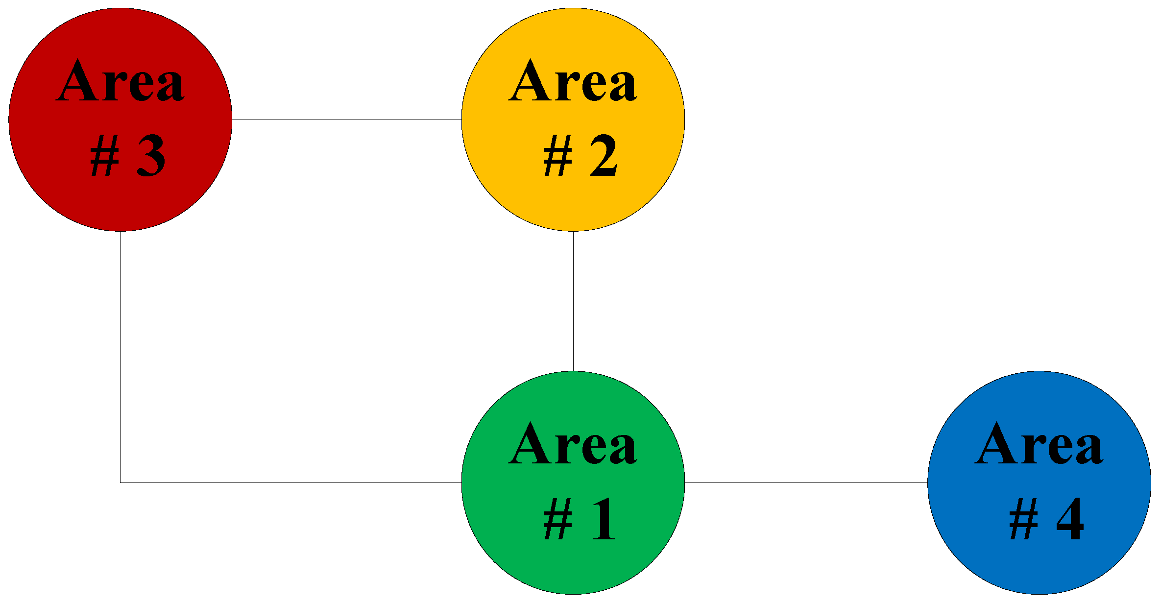
4. Power System Under Investigation

In real power systems, areas are interlinked to form one overall power system. An area can represent a single power plant with a number of generators. These several power plants are then joined to form a multi-area power system. In some cases, an area can represent a country and a number of countries can be joined to form a multi-area power system. As an example, to analyze the advantages of the proposed method, a four-area power system with non-reheated turbines is used in our simulations. The power system has been used in some research papers dealing with load frequency control [5,6]. In our case, we are applying it to estimate a disturbance in the event of a generation loss. As seen in Figure 4 Areas 1, 2 and 3 are interconnected with each other, while Area 4 is only connected with Area 1. Areas 1, 2, 3 and 4 are identical systems with non-reheated turbines. Figure 3 shows the general structure of each area. The data for the power system is given in

Table 1. Parameters of the four-area power system with non-reheated turbines.

Area No	Tt	Tg	H	D
1	0.4	0.08	0.08335	0.015
2	0.33	0.072	0.111	0.04
3	0.35	0.07	0.08	0.05
4	0.375	0.085	0.065	0.0667

.

5. Simulation Results and Discussions

The use of disturbance observers is a technique that can be used to accurately determine the magnitude of the disturbance. In this sub-section, a four-area power system with non-reheated turbines is considered. Firstly, we consider the dynamics of the single area 2. Equation (31) is used to design the disturbance observer. The system matrix A is simply a 3 × 3 matrix and neglects tie-line dynamics. Afterwards we consider the dynamics of the whole area, a 16 × 16-system matrix A is used, and it makes use of four states per area that includes the tie line dynamics.

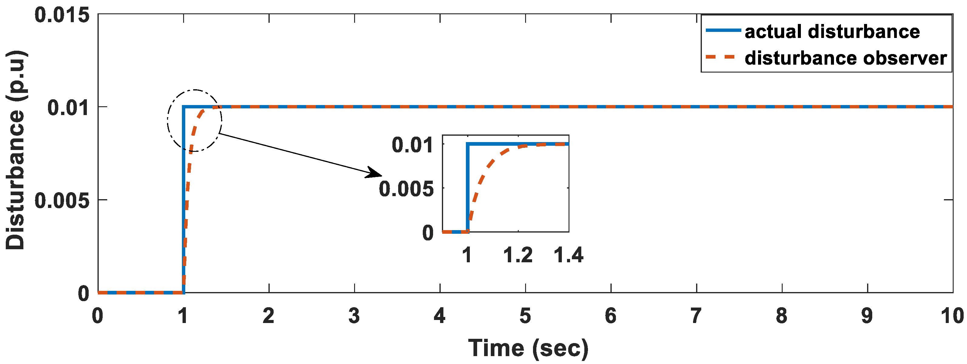
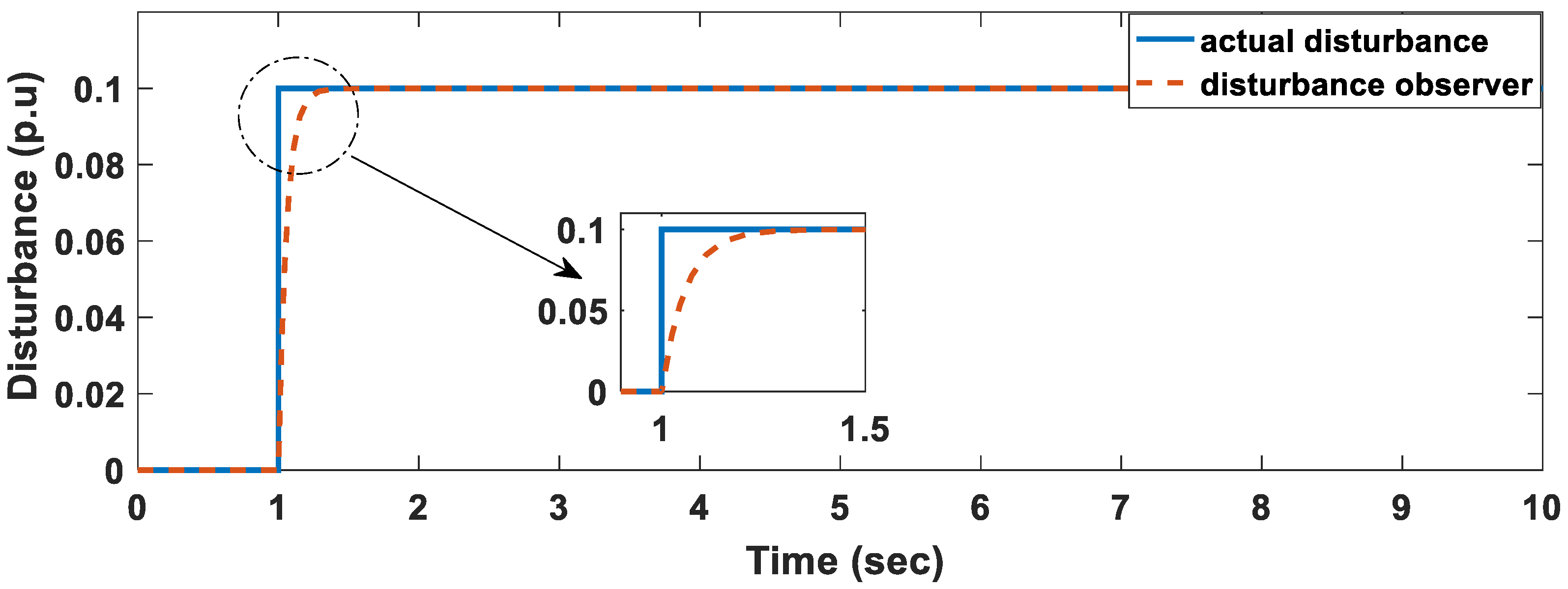
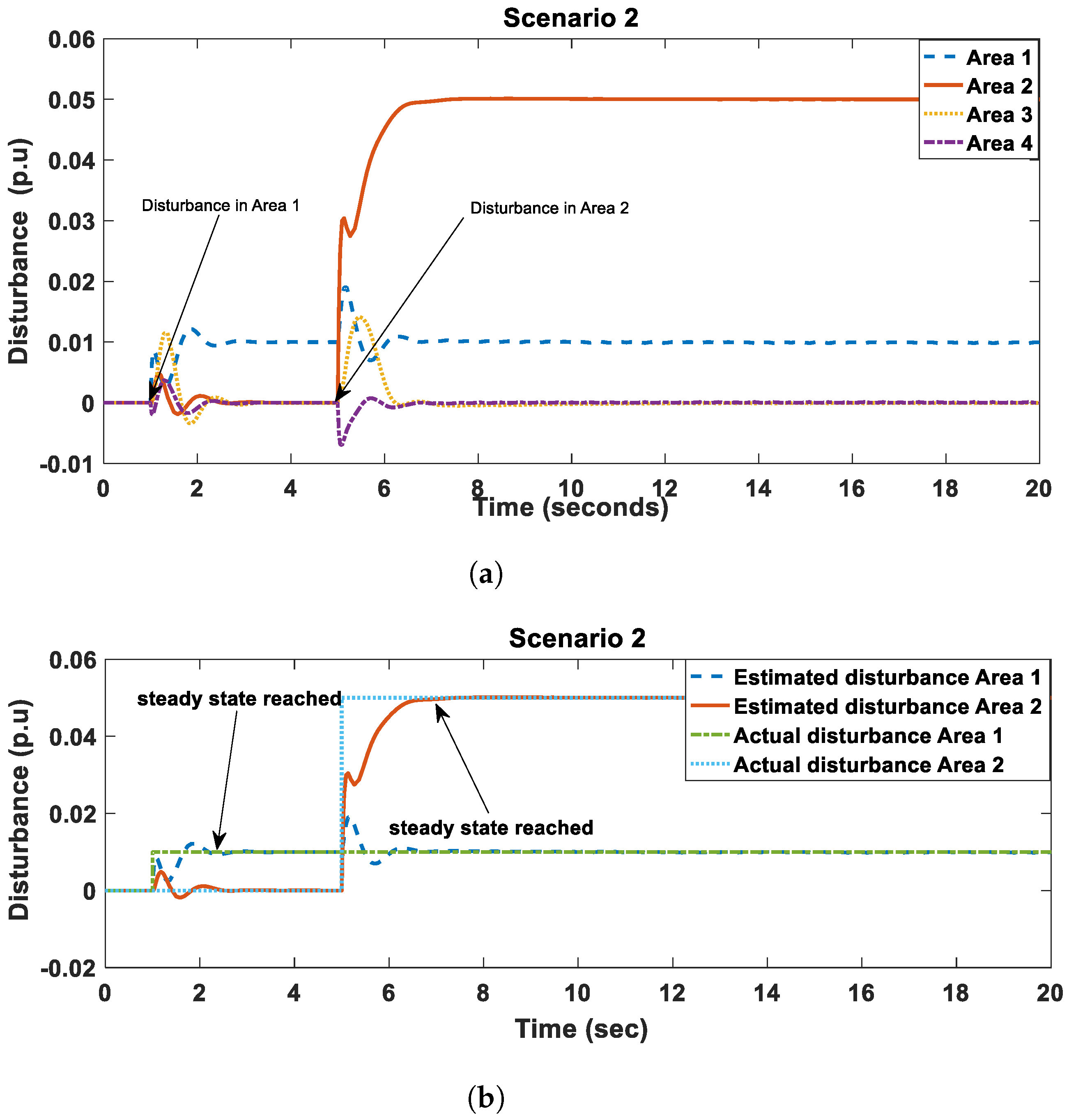
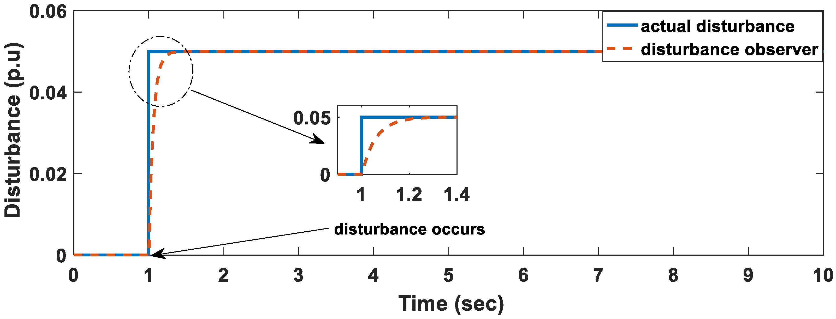
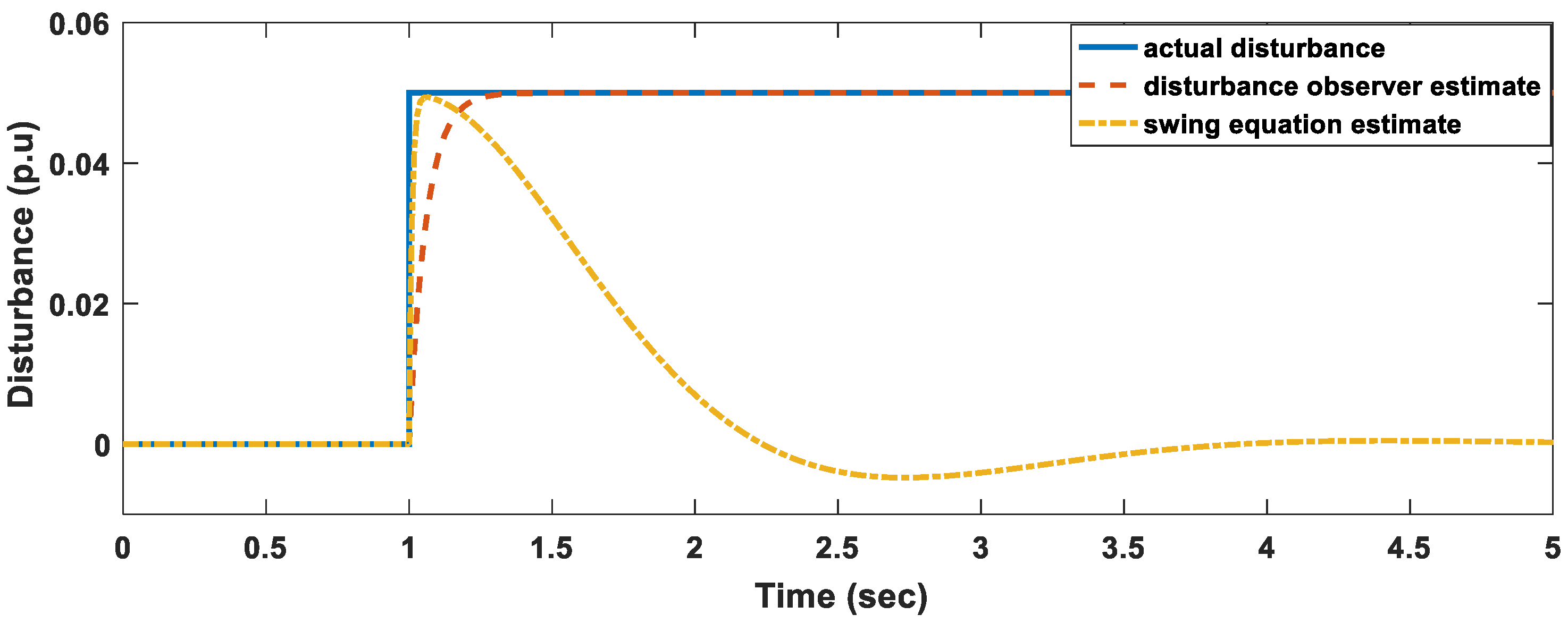
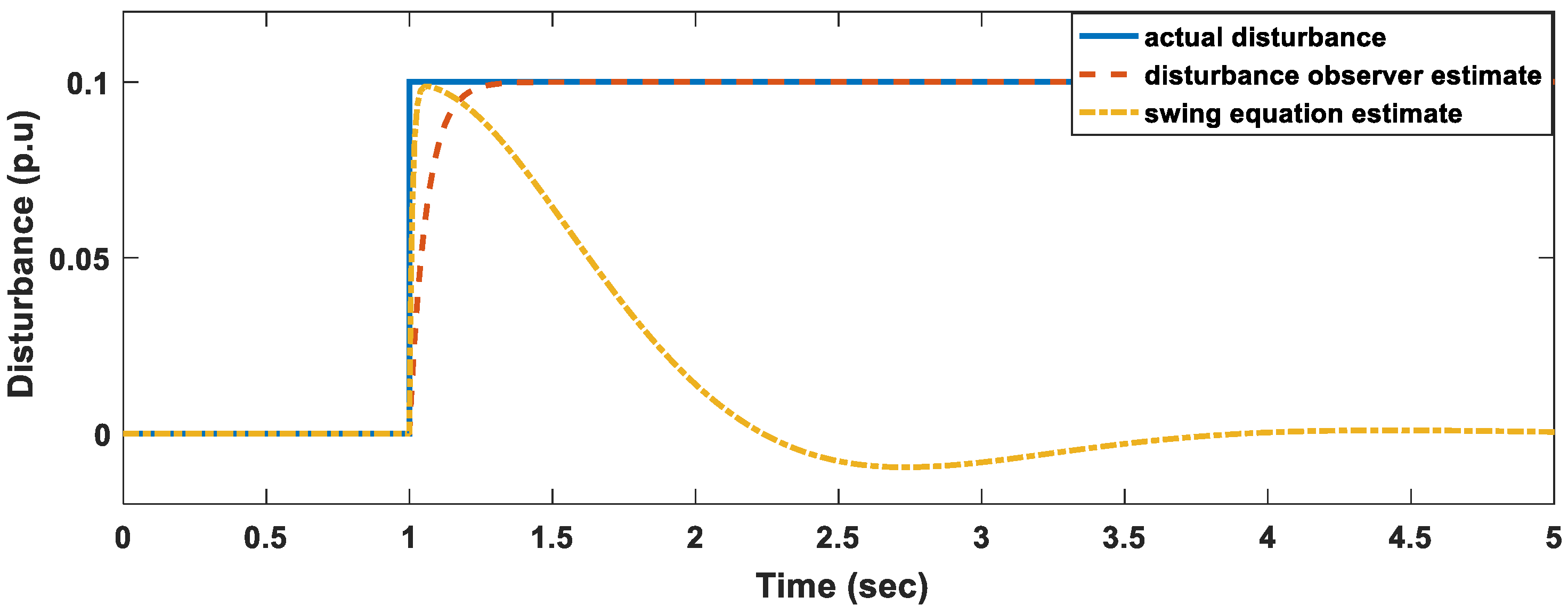
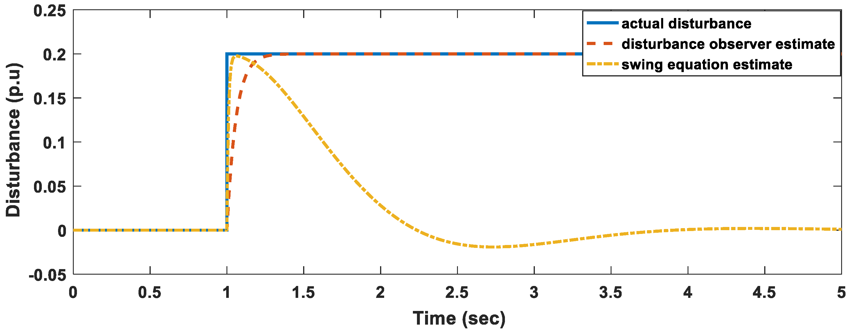
5.1. Disturbance Estimation for Single Area 2 Using the Disturbance Observer

Three disturbance scenarios are considered as follows:

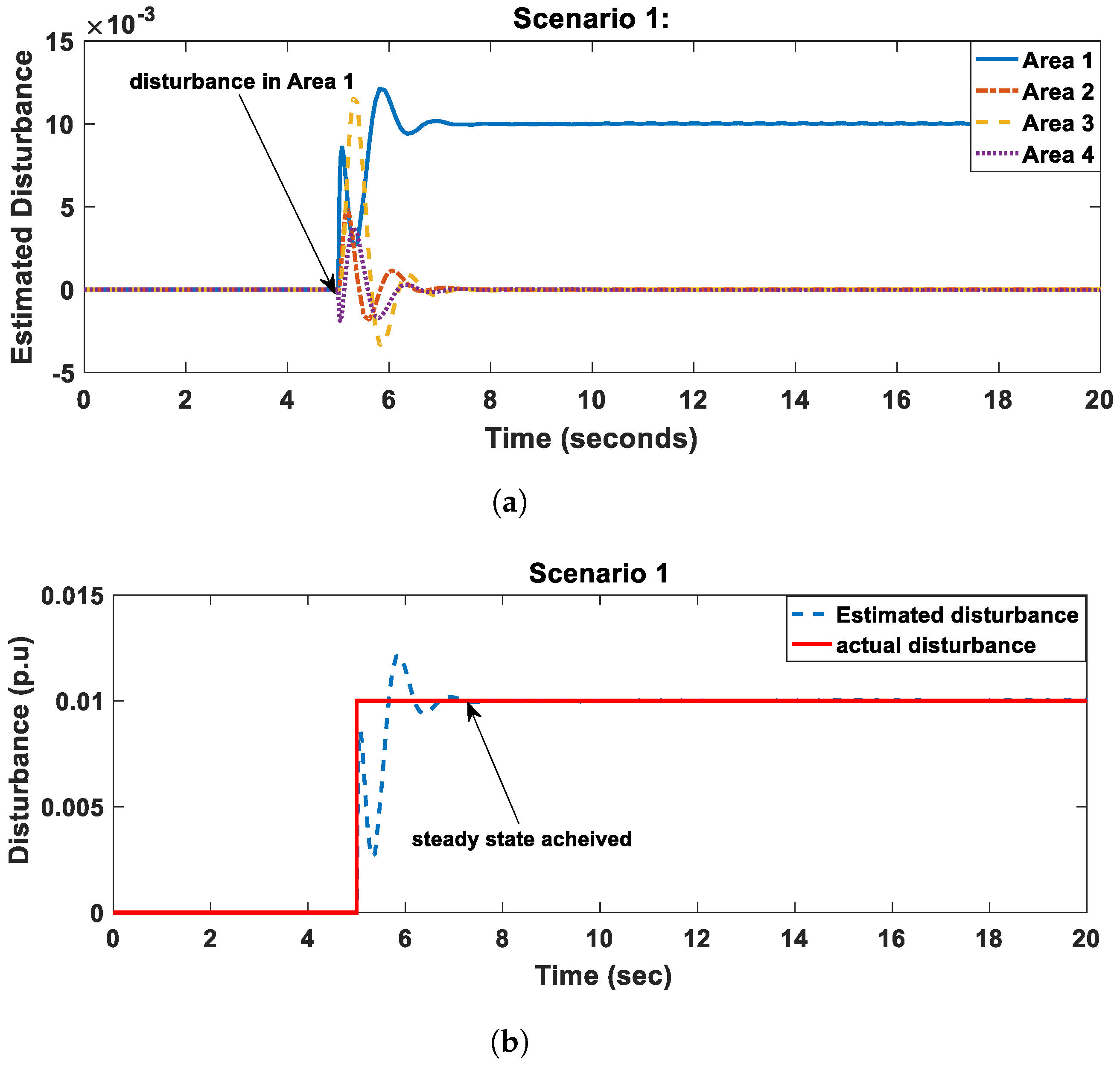
• Disturbance 1: a small disturbance (0.01 p.u),
• Disturbance 2: a medium disturbance (0.05 p.u),
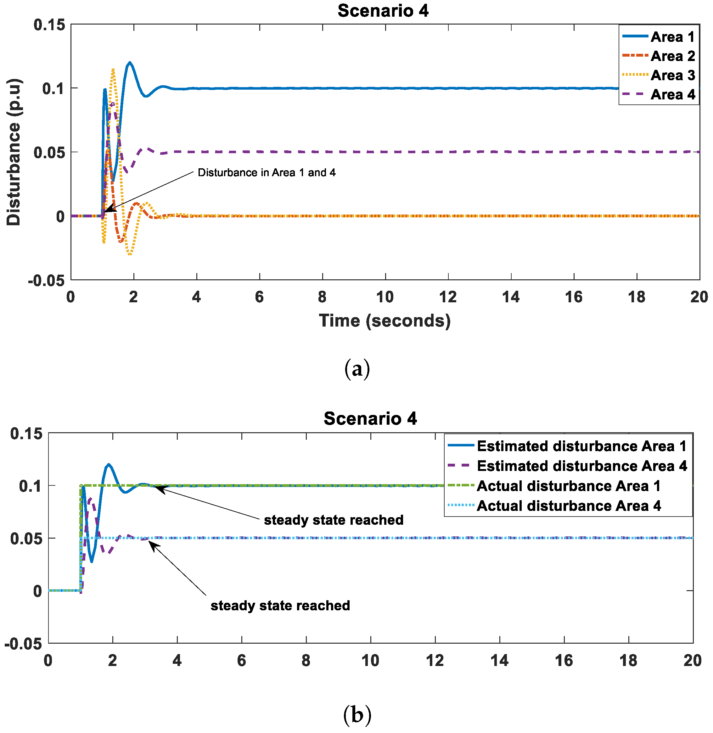
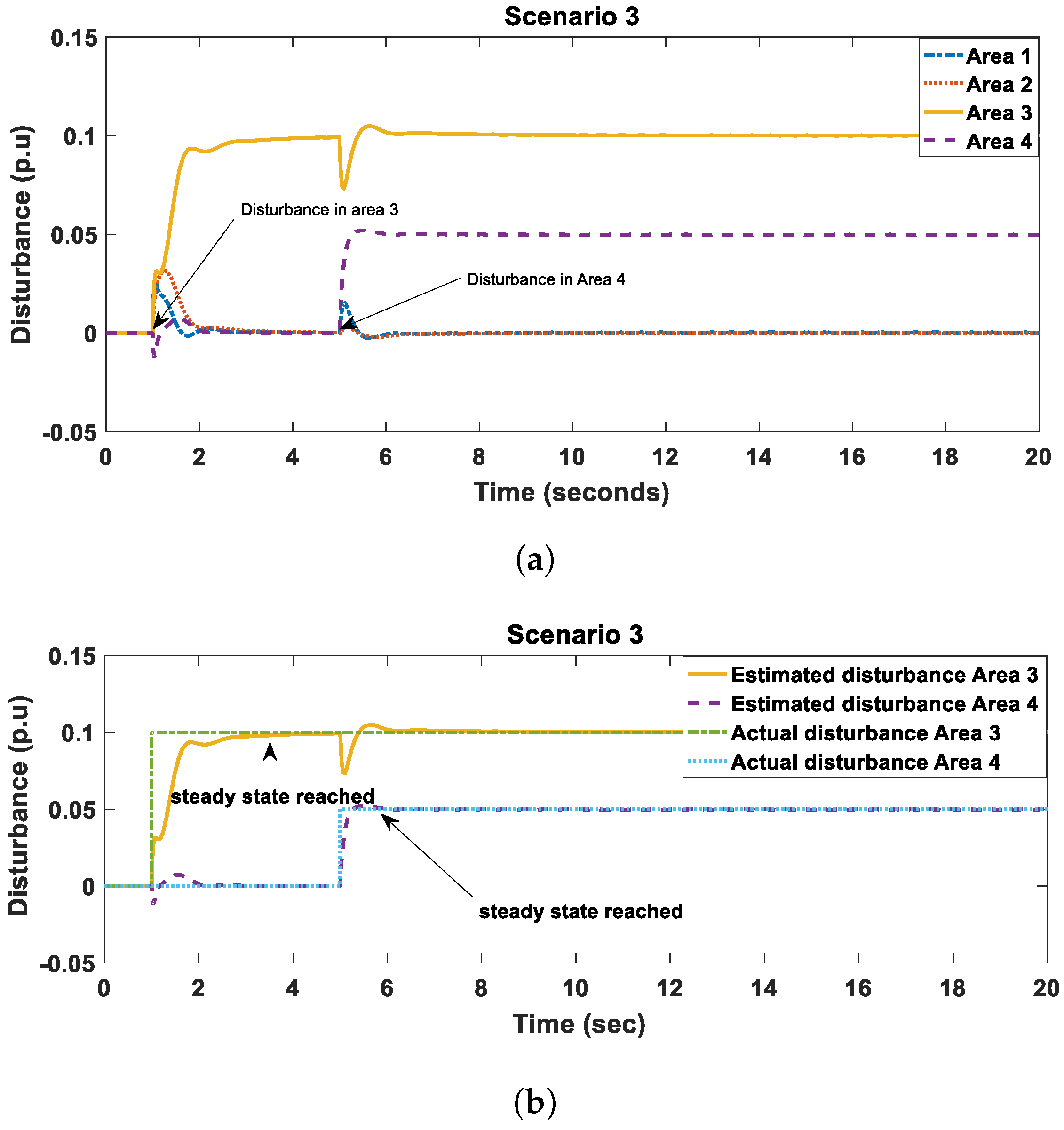
• Disturbance 3: a large disturbance (0.1 p.u).

Based on WAMS, decentralized monitoring of the power system can also be done. Here we assume that each of the four areas is under the monitoring of an operator specifically responsible for that area. We only considered the results for area 2 because we assumed that in the other three areas no disturbance occurred. In all the simulated scenarios, a disturbance occurred at $t=1$, as shown in Figure 5, Figure 6 and Figure 7. In all cases it took the disturbance observer only 0.2 s to estimate the disturbance. The estimated values were the same as the actual disturbance that occurred. This shows the superiority of disturbance observers if the system parameters are known.

5.2. Disturbance Estimation for the Whole Combined Areas Using the Disturbance Observer

In contrast to the decentralized monitoring scheme, based on WAMS, monitoring for the whole power system can also be done in real time at a control center. To achieve this a 16 × 16 matrix for the whole power system is developed. The power system matrix A and the disturbance matrix F are then used in the design of the disturbance observer. To show the efficiency of this method, four different disturbance scenarios are simulated and evaluated. The four simulated scenarios are aimed at showing that the observer can accurately estimate single disturbances and multiple disturbances occurring at the same time or at different times. From

Table 2. The disturbances and their time considered in the simulation study.

Scenario	Area#1		Area#2		Area#3		Area#4
	$\Delta {\mathit{P}}_{\mathbf{1}}$	${\mathit{t}}_{\mathbf{1}}$	$\Delta {\mathit{P}}_{\mathbf{2}}$	${\mathit{t}}_{\mathbf{2}}$	$\Delta {\mathit{P}}_{\mathbf{3}}$	${\mathit{t}}_{\mathbf{3}}$	$\Delta {\mathit{P}}_{\mathbf{4}}$	${\mathit{t}}_{\mathbf{4}}$
$S_1$	0.1	5	0	0	0	0	0	0
$S_2$	0.01	1	0.05	5	0	0	0	0
$S_3$	0	0	0	0	0.1	1	0.05	5
$S_4$	0.1	1	0	0	0	0	0.05	1

it can be seen that in scenario 1 a large disturbance of magnitude 0.1 p.u occurred only in area 1. The estimation is given in Figure 8a,b, it can be seen that the observer took approximately 2.5 s to accurately estimate the disturbance. In scenario 2, two disturbances of magnitude 0.01 p.u and 0.05 p.u occurred at $t=1$ and $t=5$ in area 1 and 2 respectively. Figure 9a,b show that it took 1.5 s to estimate disturbance in area 1 and 2.5 s in area 2.

In scenario 3 a large disturbance occurred at $t=1$ in area 3 and a medium disturbance occurred in area 4 at $t=5$. Figure 10a,b show that it took 3 s to estimate the disturbance in area 3 and less than a 1 s to estimate the disturbance in area 4. The power system under investigation is an interconnected power system consisting of several control-areas. In the aforementioned figure, a 0.1 p.u. disturbance occurred in area 3 at time $t=1$ s , then at time $t=5$ s another disturbance with magnitude of 0.05 p.u. occurred in area 4. Due to the natural interconnection between these areas by the major tie-lines, a dipping in the estimated disturbance in area 3 at $t=5$ s has occurred. This dipping would not affect the estimation and does not have bad consequences since the operator at the control center can monitor this situation and can observe the disturbances in all areas simultaneously.

Finally, in scenario 4 a large and medium disturbances occurred in area 1 and area 4 respectively, both at $t=1$. From Figure 11a,b, it took only 1.5 s in both cases to estimate the disturbance. It is also important to note that due to power line deviations in cases of two disturbance occurring at different times, the observed disturbance for the first occurred disturbance will drop then quickly return to its actual value.

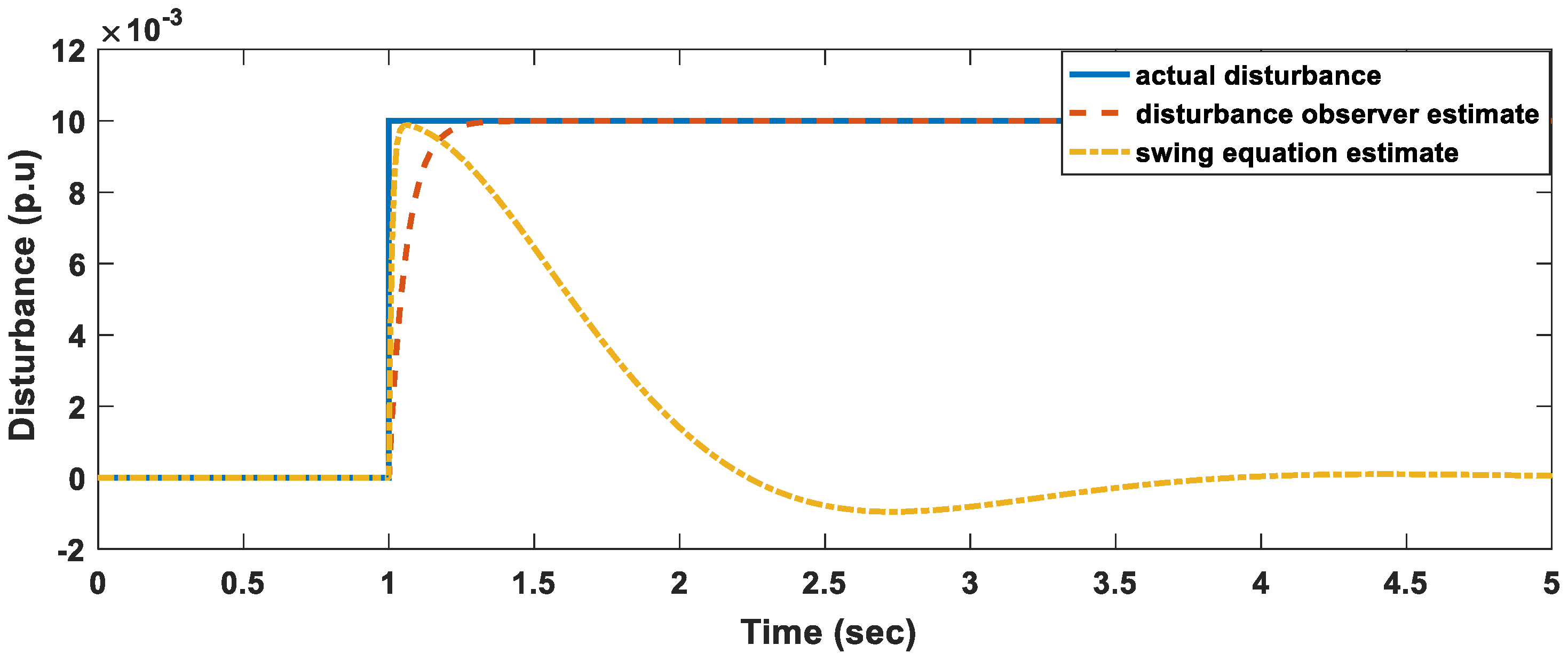
5.3. Comparison with the Existing Methods

In order to show the superiority of the disturbance observer over the swing equation, we compare three different disturbance scenarios. The swing equation is the commonly applied technique to estimate the magnitude of the power system disturbance. The equation is given as

$$\frac{2H_{i}d{f}_i}{f_{n}dt}=P_{mi}-P_{ei}=\Delta P_i$$

(34)

where $H_i$, $f_i$, $P_{mi}$, $P_{ei}$, $\Delta P_i$ and $f_n$ are the generator inertia, generator frequency, input mechanical power, output electrical power and the nominal system frequency respectively.

For comparison purposes, four disturbance scenarios are investigated as in

Table 3. Disturbance estimation using swing equation.

Scenario	Actual Disturbance	Estimated Disturbance	Error (%)
$S_1$	0.01	0.009878	1.22
$S_2$	0.05	0.049300	1.40
$S_3$	0.1	0.098200	1.80
$S_4$	0.2	0.196000	2.00

and

Table 4. Disturbance estimation using the proposed disturbance observer.

Scenario	Actual Disturbance	Estimated Disturbance	Error (%)
$S_1$	0.01	0.01	0
$S_2$	0.05	0.05	0
$S_3$	0.1	0.10	0
$S_4$	0.2	0.20	0

. In the event of a disturbance, the frequency gradient is negative, therefore, using the swing equation we would expect the disturbance magnitude to be the most negative value measured. However, in Figure 12, Figure 13, Figure 14 and Figure 15, we inverted the swing curve for comparison purposes. Table 3 shows that the greater the disturbance the greater the estimation error when using the swing equation. In scenario 1, a disturbance of 0.01 p.u magnitude occurred and the estimation error was 1.22%. For a large disturbance 0.2 p.u in scenario 4, the estimation error was 2%. Table shows the estimation results when using the disturbance observer. In all the simulated scenarios, the disturbance estimation error was 0%. In as far as disturbance estimation is concerned, the disturbance observer is superior to the swing equation.

The swing equation based method can be improved for better disturbance estimation considering the following suggestions: (i) associating the swing equation-based method with accurate online inertia estimation method, (ii) online updating the swing equation-based method with the online and accurately estimated damping coefficient, (iii) using her sapling methods and curve fitting techniques for estimating the missing data in the frequency response curve, and (iv) developing a fast method for calculating the center-of-inertia online, which can improve the disturbance estimation using the swing equation-based method.

6. Conclusions

In this paper, disturbance estimation using a disturbance observer is presented. The main advantages of the disturbance observer are: If the system parameters are close to the true values, the disturbance observer accurately estimates the disturbance. When considering single area dynamics, the response of the disturbance observer is excellent. This technique proves to be more efficient than the swing equation, especially for large disturbances. If the observer gain is properly designed, the estimation time can be significantly reduced. The disadvantages of the disturbance observer are summarized as: The disturbance observers require accurate values of the power system. When considering interconnected areas, the tie line deviations can affect the estimation speed. The presented technique can be used at the disturbance estimation stage in under frequency load shedding. For further studies, the estimated disturbance can then be used in optimization to come up with the minimum amount of load shed that exactly fits the system requirements.

References

1. Laghari, J.; Mokhlis, H.; Bakar, A.; Mohamad, H. Application of computational intelligence techniques for load shedding in power systems: A review. Energy Convers. Manag. 2013, 75, 130–140. [Google Scholar] [CrossRef]
2. Aik, D.L.H. A general-order system frequency response model incorporating load shedding: Analytic modeling and applications. IEEE Trans. Power Syst. 2006, 21, 709–717. [Google Scholar] [CrossRef]
3. Alhelou, H.H.; Golshan, M.; Fini, M.H. Wind Driven Optimization Algorithm Application to Load Frequency Control in Interconnected Power Systems Considering GRC and GDB Nonlinearities. Electr. Power Compon. Syst. 2018. [Google Scholar] [CrossRef]
4. Fini, M.H.; Yousefi, G.R.; Alhelou, H.H. Comparative study on the performance of many-objective and single-objective optimisation algorithms in tuning load frequency controllers of multi-area power systems. IET Gener. Transm. Distrib. 2016, 10, 2915–2923. [Google Scholar] [CrossRef]
5. Jones, J.R.; Kirkland, W.D. Computer algorithm for selection of frequency relays for load shedding. IEEE Comput. Appl. Power 1988, 1, 21–25. [Google Scholar] [CrossRef]
6. Wu, C.; Chen, N. Frequency-based method for fast-response reserve dispatch in isolated power systems. IEE Proc. Gener. Transm. Distrib. 2004, 151, 73–77. [Google Scholar] [CrossRef]
7. Anderson, P.M.; Fouad, A.A. Power System Control and Stability; John Wiley & Sons: Hoboken, NJ, USA, 2008. [Google Scholar]
8. Alhelou, H.; Hamedani-Golshan, M.E.; Zamani, R.; Heydarian-Forushani, E.; Siano, P. Challenges and Opportunities of Load Frequency Control in Conventional, Modern and Future Smart Power Systems: A Comprehensive Review. Energies 2018, 11, 2497. [Google Scholar] [CrossRef]
9. Alhelou, H.H.; Golshan, M. Hierarchical plug-in EV control based on primary frequency response in interconnected smart grid. In Proceedings of the 2016 24th Iranian Conference on Electrical Engineering (ICEE), Shiraz, Iran, 10–12 May 2016; pp. 561–566. [Google Scholar]
10. Alhelou, H.S.H.; Golshan, M.; Fini, M.H. Multi agent electric vehicle control based primary frequency support for future smart micro-grid. In Proceedings of the Smart Grid Conference (SGC), Tehran, Iran, 22–23 December 2015; pp. 22–27. [Google Scholar]
11. Alhelou, H.H. Fault Detection and Isolation in Power Systems Using Unknown Input Observer. In Advanced Condition Monitoring and Fault Diagnosis of Electric Machines; IGI Global: Hershey, PA, USA, 2018; p. 38. [Google Scholar]
12. Alhelou, H.H.; Golshan, M.H.; Askari-Marnani, J. Robust sensor fault detection and isolation scheme for interconnected smart power systems in presence of RER and EVs using unknown input observer. Int. J. Electr. Power Energy Syst. 2018, 99, 682–694. [Google Scholar] [CrossRef]
13. Zamani, R.; Hamedani-Golshan, M.E.; Alhelou, H.H.; Siano, P.; Pota, H.R. Islanding detection of synchronous distributed generator based on the active and reactive power control loops. Energies 2018, 11, 2819. [Google Scholar] [CrossRef]
14. Jallad, J.; Mekhilef, S.; Mokhlis, H.; Laghari, J.A. Improved UFLS with consideration of power deficit during shedding process and flexible load selection. IET Renew. Power Gener. 2018, 12, 565–575. [Google Scholar] [CrossRef]
15. Terzija, V.V. Adaptive underfrequency load shedding based on the magnitude of the disturbance estimation. IEEE Trans. Power Syst. 2006, 21, 1260–1266. [Google Scholar] [CrossRef]
16. Rudez, U.; Mihalic, R. Monitoring the first frequency derivative to improve adaptive underfrequency load-shedding schemes. IEEE Trans. Power Syst. 2011, 26, 839–846. [Google Scholar] [CrossRef]
17. Ketabi, A.; Fini, M.H. An underfrequency load shedding scheme for hybrid and multiarea power systems. IEEE Trans. Smart Grid 2015, 6, 82–91. [Google Scholar] [CrossRef]
18. Tofis, Y.; Timotheou, S.; Kyriakides, E. Minimal load shedding using the swing equation. IEEE Trans. Power Syst. 2017, 32, 2466–2467. [Google Scholar] [CrossRef]
19. Alhelou, H.H. An Overview of Wide Area Measurement System and Its Application in Modern Power Systems. In Handbook of Research on Smart Power System Operation and Control; IGI Global: Hershey, PA, USA, 2019; pp. 289–307. [Google Scholar]
20. Alhelou, H.H. Under Frequency Load Shedding Techniques for Future Smart Power Systems. In Handbook of Research on Smart Power System Operation and Control; IGI Global: Hershey, PA, USA, 2019; pp. 188–202. [Google Scholar]
21. Mahfoud, F.; Guzun, B.D.; Lazaroiu, G.C.; Alhelou, H.H. Power Quality of Electrical Power Systems. In Handbook of Research on Smart Power System Operation and Control; IGI Global: Hershey, PA, USA, 2019; pp. 265–288. [Google Scholar]
22. Makdisie, C.; Haidar, B.; Alhelou, H.H. An Optimal Photovoltaic Conversion System for Future Smart Grids. In Handbook of Research on Power and Energy System Optimization; IGI Global: Hershey, PA, USA, 2018; pp. 601–657. [Google Scholar]
23. Chang-Chien, L.R.; An, L.N.; Lin, T.W.; Lee, W.J. Incorporating demand response with spinning reserve to realize an adaptive frequency restoration plan for system contingencies. IEEE Trans. Smart Grid 2012, 3, 1145–1153. [Google Scholar] [CrossRef]
24. Sattinger, W. Application of PMU measurements in Europe TSO approach and experience. In Proceedings of the 2011 IEEE Trondheim PowerTech, Trondheim, Norway, 19–23 June 2011; pp. 1–4. [Google Scholar]
25. Hauer, J.F.; Mittelstadt, W.A.; Martin, K.E.; Burns, J.W.; Lee, H.; Pierre, J.W.; Trudnowski, D.J. Use of the WECC WAMS in wide-area probing tests for validation of system performance and modeling. IEEE Trans. Power Syst. 2009, 24, 250–257. [Google Scholar] [CrossRef]
26. Terzija, V.V.; Valverde, G.; Cai, D.; Regulski, P.; Madani, V.; Fitch, J.; Skok, S.; Begovic, M.; Phadke, A.G. Wide-area monitoring, protection, and control of future electric power networks. Proc. IEEE 2011, 99, 80–93. [Google Scholar] [CrossRef]
27. Hauer, J.; Hughes, F.J.; Trudnowski, D.; Rogers, G.; Pierre, J.; Scharf, L.; Litzenberger, W. A Dynamic Information Manager for Networked Monitoring of Large Power Systems; EPRI Report TR-112031; BPA and PNNL: Palo Alto, CA, USA, 1999. [Google Scholar]
28. Kamwa, I.; Grondin, R. PMU configuration for system dynamic performance measurement in large, multiarea power systems. IEEE Trans. Power Syst. 2002, 17, 385–394. [Google Scholar] [CrossRef]
29. Zhong, Z.; Xu, C.; Billian, B.J.; Zhang, L.; Tsai, S.J.; Conners, R.W.; Centeno, V.A.; Phadke, A.G.; Liu, Y. Power system frequency monitoring network (FNET) implementation. IEEE Trans. Power Syst. 2005, 20, 1914–1921. [Google Scholar] [CrossRef]
30. La Scala, M.; De Benedictis, M.; Bruno, S.; Grobovoy, A.; Bondareva, N.; Borodina, N.; Denisova, D.; Germond, A.; Cherkaoui, R. Development of applications in WAMS and WACS: An international cooperation experience. In Proceedings of the 2006 IEEE Power Engineering Society General Meeting, Montreal, QC, Canada, 18–22 June 2006; p. 10. [Google Scholar]
31. Sarailoo, M.; Wu, N.E. Cost-Effective Upgrade of PMU Networks for Fault-Tolerant Sensing. IEEE Trans. Power Syst. 2018, 33, 3052–3063. [Google Scholar] [CrossRef]
32. Liao, K.; Xu, Y. A robust load frequency control scheme for power systems based on second-order sliding mode and extended disturbance observer. IEEE Trans. Ind. Inform. 2018, 14, 3076–3086. [Google Scholar] [CrossRef]
33. Machowski, J.; Janus, W.; Bumby, J.R. Power System Dynamics: Stability and Control; John Wiley & Sons: Hoboken, NJ, USA, 2011. [Google Scholar]
34. Wang, G.; Xin, H.; Gan, D.; Li, N.; Wang, Z. An investigation into WAMS-based Under-frequency load shedding. In Proceedings of the 2012 IEEE Power and Energy Society General Meeting, San Diego, CA, USA, 22–26 July 2012; pp. 1–7. [Google Scholar]
35. Shi, Q.; Li, F.F.; Cui, H. Analytical Method to Aggregate Multi-Machine SFR Model with Applications in Power System Dynamic Studies. IEEE Trans. Power Syst. 2018, 33, 6355–6367. [Google Scholar] [CrossRef]
36. Han, H.; Gao, S.; Shi, Q.; Cui, H.; Li, F. Security-based active demand response strategy considering uncertainties in power systems. IEEE Access 2017, 5, 16953–16962. [Google Scholar] [CrossRef]
37. Liu, F.; Li, Y.; Cao, Y.; She, J.; Wu, M. A two-layer active disturbance rejection controller design for load frequency control of interconnected power system. IEEE Trans. Power Syst. 2016, 31, 3320–3321. [Google Scholar] [CrossRef]
38. Singh, V.P.; Kishor, N.; Samuel, P. Distributed multi-agent system-based load frequency control for multi-area power system in smart grid. IEEE Trans. Ind. Electron. 2017, 64, 5151–5160. [Google Scholar] [CrossRef]
Figure 1. System frequency response (SFR) model with non-reheat turbines.
Applsci 09 00990 g001
Figure 2. Set up for disturbance estimation.
Applsci 09 00990 g002
Figure 3. Disturbance observer block-diagram.
Applsci 09 00990 g003
Figure 4. Four-area power system under investigation.
Applsci 09 00990 g004
Figure 5. Estimated and actual disturbance for scenario 1.
Applsci 09 00990 g005
Figure 6. Estimated and actual disturbance for scenario 2.
Applsci 09 00990 g006
Figure 7. Estimated and actual disturbance for scenario 3.
Applsci 09 00990 g007
Figure 8. Scenario 1: (a) estimated disturbances and (b) actual vs. estimated disturbances.
Applsci 09 00990 g008
Figure 9. Scenario 2: (a) estimated disturbances and (b) actual vs. estimated disturbances.
Applsci 09 00990 g009
Figure 10. Scenario 3: (a) estimated disturbances and (b) actual vs. estimated disturbances.
Applsci 09 00990 g010
Figure 11. Scenario 4: (a) estimated disturbances and (b) actual vs. estimated disturbances.
Applsci 09 00990 g011
Figure 12. Scenario 1 disturbance observer vs swing equation estimation.
Applsci 09 00990 g012
Figure 13. Scenario 2 disturbance observer vs swing equation estimation.
Applsci 09 00990 g013
Figure 14. Scenario 3 disturbance observer vs swing equation estimation.
Applsci 09 00990 g014
Figure 15. Scenario 4 disturbance observer vs swing equation estimation.
Applsci 09 00990 g015