A Photon Blockade in a Coupled Cavity System Mediated by an Atom

Abstract
1. Introduction
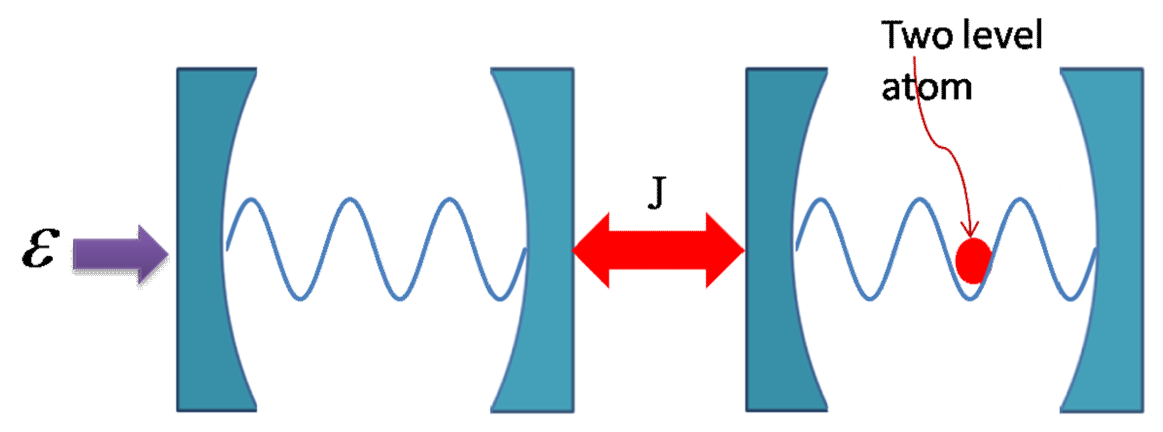
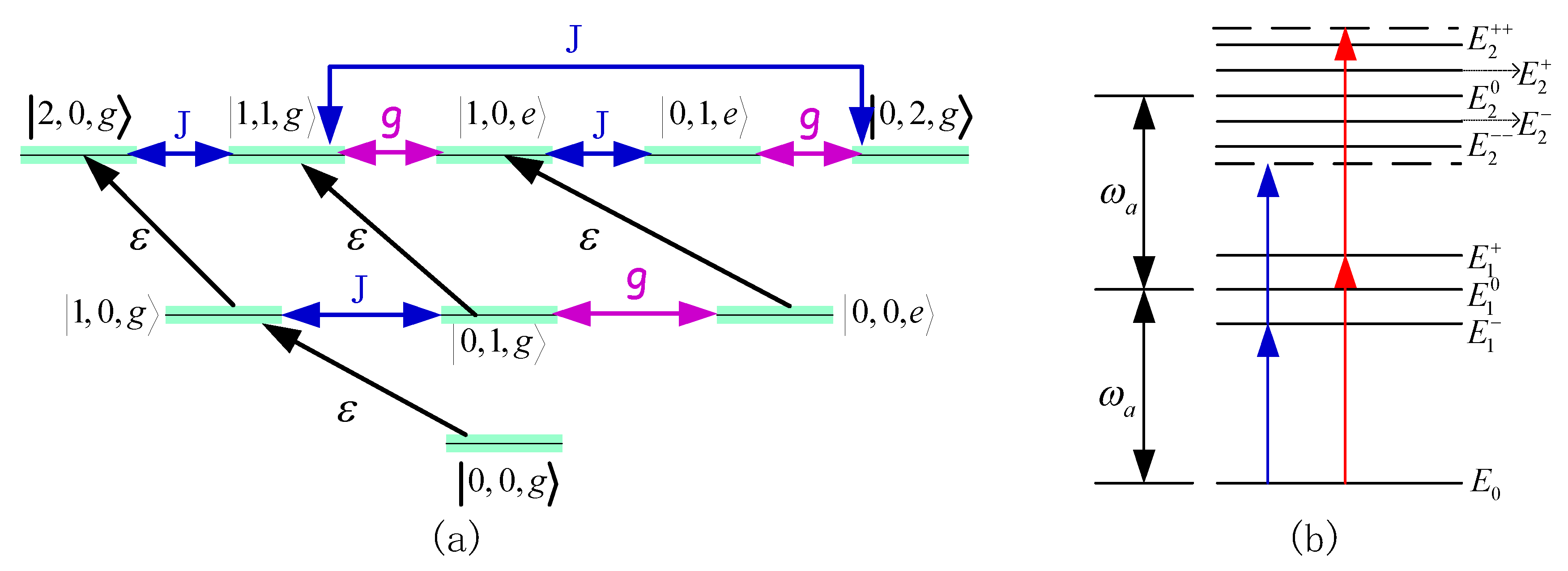
2. Model
3. Numerical Computation Conventional and Unconventional Photon Blockade
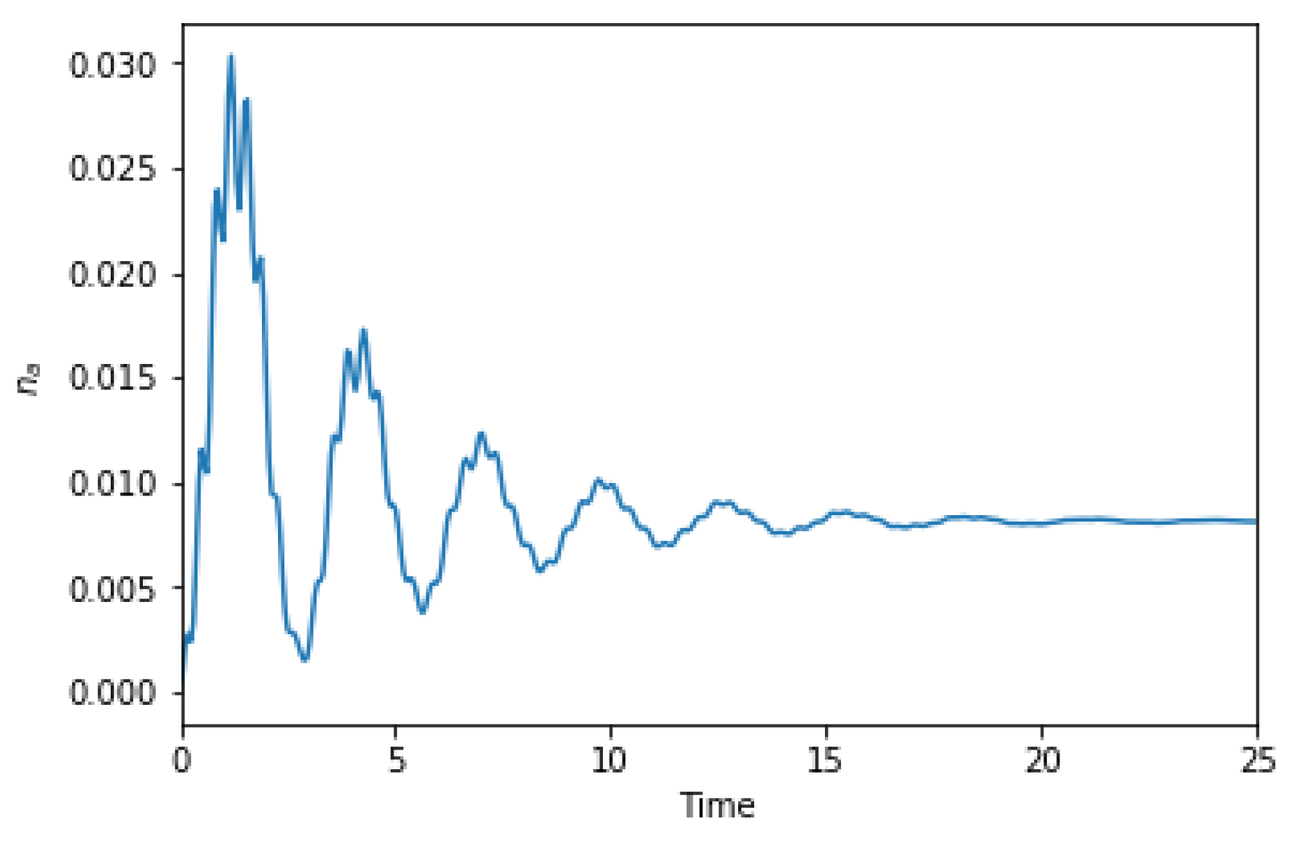
3.1. Quantum Master Equation
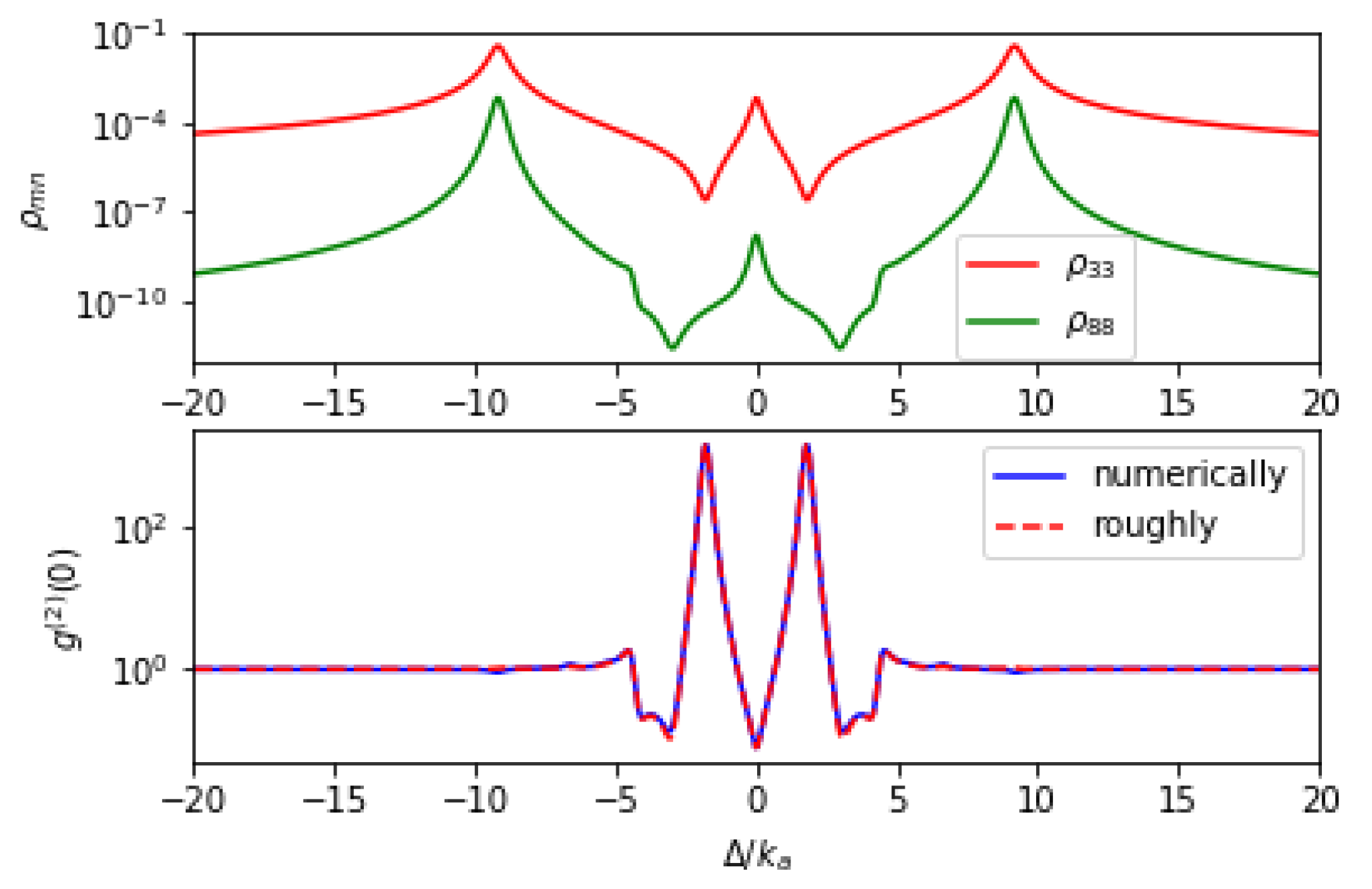
3.2. Unconventional Photon Blockade with Atom-Cavity Detuning
4. Optimal Parameters for Sub-Poissonian Characters Derived by the Non-Hermitian Effective Hamiltonian Method
5. Supplementary Discussion
6. Conclusions
Author Contributions
Funding
Conflicts of Interest
References
- Hadfield, R.H. Single-photon detectors for optical quantum information applications. Nat. Photonics 2009, 3, 696–705. [Google Scholar] [CrossRef]
- Eisaman, M.D.; Fan, J.; Migdall, A.; Polyakov, S.V. Invited review article: Single-photon sources and detectors. Rev. Sci. Instrum. 2011, 82, 071101. [Google Scholar] [CrossRef] [PubMed]
- Lounis, B.; Orrit, M. Single-photon sources. Rep. Prog. Phys. 2005, 68, 1129–1179. [Google Scholar] [CrossRef]
- Clauser, J.F. Experimental distinction between the quantum and classical field-theoretic predictions for the photoelectric effect. Phys. Rev. D 1974, 9, 853. [Google Scholar] [CrossRef]
- Diedrich, F.; Walther, H. Nonclassical radiation of a single stored ion. Phys. Rev. Lett. 1987, 58, 203–206. [Google Scholar] [CrossRef] [PubMed]
- De Martini, F.; Di Giuseppe, G.; Marrocco, M. Single-mode generation of quantum photon states by excited single molecules in a microcavity trap. Phys. Rev. Lett. 1996, 76, 900–903. [Google Scholar] [CrossRef] [PubMed]
- Lounis, B.; Moerner, W.E. Single photons on demand from a single molecule at room temperature. Nature 2000, 407, 491–493. [Google Scholar] [CrossRef]
- Brouri, R.; Beveratos, A.; Poizat, J.P.; Grangier, P. Photon antibunching in the fluorescence of individual color centers in diamond. Opt. Lett. 2000, 25, 1294–1296. [Google Scholar] [CrossRef]
- Michler, P.; Imamoğlu, A.; Mason, M.D.; Carson, P.J.; Strouse, G.F.; Buratto, S.K. Quantum correlation among photons from a single quantum dot at room temperature. Nature 2000, 406, 968–970. [Google Scholar] [CrossRef]
- He, Y.M.; He, Y.; Wei, Y.J.; Wu, D.; Atatüre, M.; Schneider, C.; Höfling, S.; Kamp, M.; Lu, C.Y.; Pan, J.W. On-demand semiconductor single-photon source with near-unity indistinguishability. Nat. Nanotechnol. 2013, 8, 213–217. [Google Scholar] [CrossRef]
- Gschrey, M.; Thoma, A.; Schnauber, P.; Seifried, M.; Schmidt, R.; Wohlfeil, B.; Krüger, L.; Schulze, J.H.; Heindel, T.; Burger, S.; et al. Highly indistinguishable photons from deterministic quantum-dot microlenses utilizing three-dimensional in situ electron-beam lithography. Nat. Commun. 2015, 6, 7662. [Google Scholar] [CrossRef] [PubMed]
- Imamoḡlu, A.; Schmidt, H.; Woods, G.; Deutsch, M. Strongly interacting photons in a nonlinear cavity. Phys. Rev. Lett. 1997, 79, 1467. [Google Scholar] [CrossRef]
- Leoński, W.; Tanaś, R. Possibility of producing the one-photon state in a kicked cavity with a nonlinear Kerr medium. Phys. Rev. A 1994, 49, R20–R23. [Google Scholar] [CrossRef] [PubMed]
- Birnbaum, K.M.; Boca, A.; Miller, R.; Boozer, A.D.; Northup, T.E.; Kimble, H.J. Photon blockade in an optical cavity with one trapped atom. Nature 2005, 436, 87–90. [Google Scholar] [CrossRef] [PubMed]
- Peyronel, T.; Firstenberg, O.; Liang, Q.Y.; Hofferberth, S.; Gorshkov, A.V.; Pohl, T.; Lukin, M.D.; Vuletić, V. Quantum nonlinear optics with single photons enabled by strongly interacting atoms. Nature 2012, 488, 57–60. [Google Scholar] [CrossRef] [PubMed]
- Liew, T.C.H.; Savona, V. Single photons from coupled quantum modes. Phys. Rev. Lett. 2010, 104, 183601. [Google Scholar] [CrossRef] [PubMed]
- Flayac, H.; Savona, V. Unconventional photon blockade. Phys. Rev. A 2017, 96, 053810. [Google Scholar] [CrossRef]
- Bin, Q.; Lü, X.Y.; Bin, S.W.; Wu, Y. Two-photon blockade in a cascaded cavity-quantum-electrodynamics system. Phys. Rev. A 2018, 98, 043858. [Google Scholar] [CrossRef]
- Bamba, M.; Imamoğlu, A.; Carusotto, I.; Ciuti, C. Origin of strong photon antibunching in weakly nonlinear photonic molecules. Phys. Rev. A 2011, 83, 021802. [Google Scholar] [CrossRef]
- Zou, F.; Lai, D.G.; Liao, J.Q. Photon blockade effect in a coupled cavity system. arXiv, 2018; arXiv:1803.06642. [Google Scholar]
- Xu, X.W.; Li, Y. Tunable photon statistics in weakly nonlinear photonic molecules. Phys. Rev. A 2014, 90, 043822. [Google Scholar] [CrossRef]
- Shen, H.Z.; Zhou, Y.H.; Yi, X.X. Tunable photon blockade in coupled semiconductor cavities. Phys. Rev. A 2015, 91, 063808. [Google Scholar] [CrossRef]
- Flayac, H.; Gerace, D.; Savona, V. An all-silicon single-photon source by unconventional photon blockade. Sci. Rep. 2015, 5, 11223. [Google Scholar] [CrossRef] [PubMed]
- Gerace, D.; Savona, V. Unconventional photon blockade in doubly resonant microcavities with second-order nonlinearity. Phys. Rev. A 2014, 89, 031803. [Google Scholar] [CrossRef]
- Tang, J.; Geng, W.; Xu, X. Quantum interference induced photon blockade in a coupled single quantum dot-cavity system. Sci. Rep. 2015, 5, 9252. [Google Scholar] [CrossRef] [PubMed]
- Carmichael, H. Master equations and source. In An Open Systems Approach to Quantum Optics; Springer: Berlin/Heidelberg, Germany, 1993; pp. 22–35. [Google Scholar]
- Breuer, H.P.; Petruccione, F. Quantum master equations. In The Theory of Open Quantum Systems; Oxford University Press: Oxford, UK, 2002; pp. 109–216. [Google Scholar]
- Carmichael, H.J. Quantum trajectory theory for cascaded open systems. Phys. Rev. Lett. 1993, 70, 2273–2276. [Google Scholar] [CrossRef] [PubMed]
- Johansson, J.R.; Nation, P.D.; Nori, F. QuTiP: An open-source Python framework for the dynamics of open quantum systems. Comput. Phys. Commun. 2012, 183, 1760–1772. [Google Scholar] [CrossRef]
- Carmichael, H.J.; Brecha, R.J.; Rice, P.R. Quantum interference and collapse of the wavefunction in cavity QED. Opt. Commun. 1991, 82, 73–79. [Google Scholar] [CrossRef]


© 2019 by the authors. Licensee MDPI, Basel, Switzerland. This article is an open access article distributed under the terms and conditions of the Creative Commons Attribution (CC BY) license (http://creativecommons.org/licenses/by/4.0/).
Share and Cite
Li, M.-C.; Chen, A.-X. A Photon Blockade in a Coupled Cavity System Mediated by an Atom. Appl. Sci. 2019, 9, 980. https://doi.org/10.3390/app9050980
Li M-C, Chen A-X. A Photon Blockade in a Coupled Cavity System Mediated by an Atom. Applied Sciences. 2019; 9(5):980. https://doi.org/10.3390/app9050980
Chicago/Turabian StyleLi, Ming-Cui, and Ai-Xi Chen. 2019. "A Photon Blockade in a Coupled Cavity System Mediated by an Atom" Applied Sciences 9, no. 5: 980. https://doi.org/10.3390/app9050980
APA StyleLi, M.-C., & Chen, A.-X. (2019). A Photon Blockade in a Coupled Cavity System Mediated by an Atom. Applied Sciences, 9(5), 980. https://doi.org/10.3390/app9050980