Laboratory Observations of Repeated Interactions between Ruptures and the Fault Bend Prior to the Overall Stick-Slip Instability Based on a Digital Image Correlation Method

Abstract

Fault geometry plays important roles in the evolution of earthquake ruptures. Experimental studies on the spatiotemporal evolution of the ruptures of a fault with geometric bands are important for understanding the effects of the fault bend on the seismogenic process. However, the spatial sampling of the traditional point contact type sensors is quite low, which is unable to observe the detailed spatiotemporal evolution of ruptures. In this study, we use a high-speed camera combined with a digital image correlation (DIC) method to observe ruptures during stick-slip motions of a simulated bent fault. Meanwhile, strain gages were also used to test the results of the DIC method. Multiple cycles of the alternative propagation of ruptures between the two fault segments on the both sides of the fault bend were observed prior to the overall failure of the fault. Moreover, the slip velocity and rupture speed were observed getting higher during this process. These results indicate the repeated interactions between the ruptures and the fault bend prior to the overall instability of the fault, which distinguishes the effect of the fault bend from the effect of asperities in straight faults on the evolution of ruptures. In addition, improvement in the temporal sampling rate of the DIC measurement system may further help to unveil the rupture evolution during the overall instability in future.

1. Introduction

The experimental study of the evolution of earthquake ruptures is of great significance for understanding the underlying physical process of earthquake preparation and occurrence. Geological surveys and field observation data showed that fault geometry plays important roles in the initiation and propagation of earthquake ruptures [1,2,3,4,5,6,7,8]. Numerical simulations analyzed the influences of the fault bend on the rupture process and the fault slip distribution, which revealed that the angle of the fault bend, the normal stress, and the loading mode play important roles in the initiation and propagation of the ruptures [9,10,11,12,13,14]. Specifically, the rupture zone and overall slip distribution on the fault are controlled by the angle of the fault bend, while rupture velocity and detailed slip distribution around the bend are influenced by time-dependent normal stress changes caused by the rupture [12]. The fault bend will serve as an initiation and/or a termination point for the rupture via reducing normal stress on the dilatational segment and increasing normal stress on the compressive segment of the bent fault during dynamic ruptures [11]. The angle of the fault bend and the sliding direction of a dip-slip bent fault control the time and location of the rupture nucleation [13]. In addition, the rupture process of the Chi-Chi earthquake [10,15], Landers earthquake [16], and İzmit earthquake [17] were reconstructed via numerical simulations to further reveal the mechanism of the influence of fault geometry on the earthquake rupture process using seismic and geodetic data combined with bent fault models.

Physical experiments have been carried out to study the rupture process and the evolution of the relevant physical fields of bent faults. It was observed that the two segments on each side of the fault bend became active alternatively during sliding, which implied that the fault bend plays a role of a valve during sliding [18]; a two-step rupture propagation process was observed prior to the overall instability of the fault. Namely, the dynamic rupture started on a fault segment is stopped near the fault bend, which is restarted near the bend on the other fault segment after a certain delay time and leads to the overall slip of the entire fault without being arrested by the presence of the fault bend [19]. The influence of fault bends on the growth of sub-Rayleigh and intersonic dynamic shear ruptures was also studied in the laboratory [20]. In addition, the changes and characteristics of the deformation fields before and after the instability of the bent faults were also studied in the laboratory [21,22,23,24].

From the above results based on experiments conducted in rock materials [18,19,21,22,23,24], alternative activities were observed between the two fault segments on both sides of the bend before the overall instability of the fault. Since these experimental results were obtained via point contact type observation methods, such as strain gages, the spatial sampling was quite sparse. As a result, the detailed spatiotemporal evolution of ruptures cannot be observed. Accordingly, at least two problems remain unclear: (1) Is there only one alternative propagation of ruptures between the two fault segments on both sides of the bend prior to the overall instability of the fault as proposed in [19]? (2) What is the characteristic of the ruptures during their alternative propagation between the two fault segments? The solution to the two problems depends on the observation of the detailed spatiotemporal evolution of the ruptures. Therefore, it is necessary to further study the rupture evolution of the bent fault using high spatiotemporal sampling observation methods.

An experimental study depends strongly on observations. Quantitative measurement of fault slip, slip velocity, and strain via intensive sampling in time and space is very important to reveal the detailed spatiotemporal evolution of fault ruptures. The observation methods for fault slip and deformation can be divided into contact type (such as resistance strain gages or displacement gages) and non-contact type (e.g., the digital image correlation method). The contact type observation requires the sensors to be in contact with the sample, while the non-contact type observation allows the sensor to be separated from the sample. The contact type sensor occupies a certain area, which limits the number of sensors used in measurement. For instance, only dozens of strain gages can be used to cover a fault of tens of centimeters long, which were usually used in previous experimental studies [18,19,21,22,23,24]. However, via the digital image correlation (DIC) method, thousands of pixels can be used by camera photography to observe the slip and deformation along a fault of equivalent length [25,26,27,28,29,30]. Therefore, compared with the contact type observation, the spatial sampling rate of the DIC method is dramatically higher. On the other hand, the measurement precision of the contact type sensor is usually higher than that of the non-contact type sensor. For example, the measurement precision of the strain gage can easily reach 1 µε (micro-strain) [23], which is difficult to achieve by the DIC method. Therefore, it will be effective and economical for measurements to comprehensively utilize the two types of observations via making their respective advantages and verifying the results of each other.

Thus, the DIC method combined with strain gages are used in this study to observe the detailed spatiotemporal evolution of ruptures along a bent fault.

2. Materials and Methods

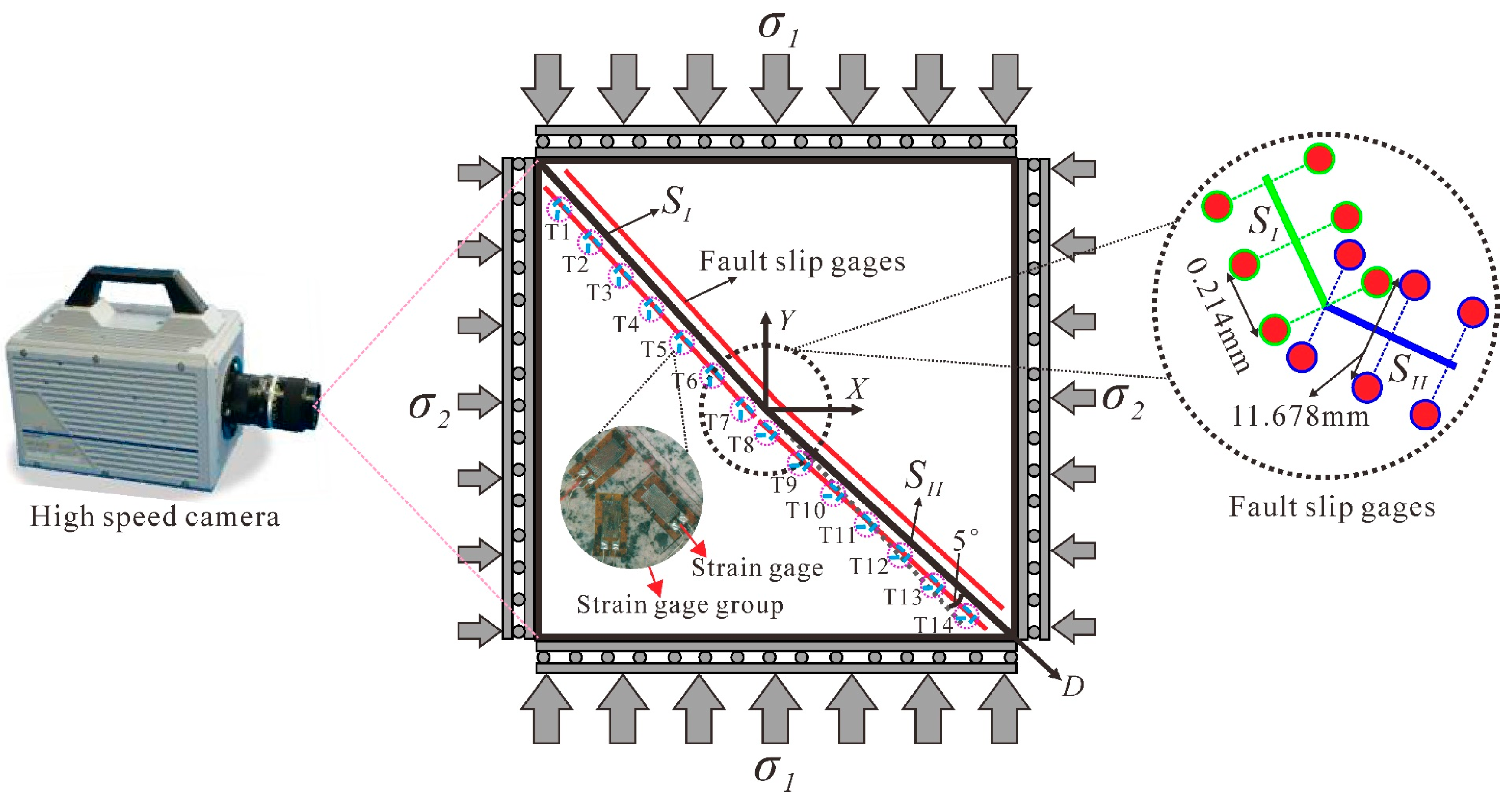
2.1. Sample and Loading Conditions

Most of the devastating earthquakes are located in the upper crust, which has a granodioritic bulk composition [31]. Therefore, the use of the granodiorite as a sample to simulate the earthquake rupture process is representative. A granodiorite sample with size of 300 × 300 × 50 mm was cut through to form a bent fault. The fault surface was ground with a diamond wheel with a particle size of 150#. The roughness of the fault surface was ~100 µm before loading. The elastic modulus, Poisson’s ratio, and shear modulus of the sample were 60 GPa, 0.27, and 24 GPa, respectively, which were tested via a uniaxial press machine. As shown in Figure 1, the bend point divided the fault into two segments of equal length. The segment with a small angle (42.5°) from the direction of σ₁ was referred to as segment S_I, while the other segment with a larger angle (47.5°) from the direction of σ₁ was referred to as segment S_II. The angle between the two segments was 5°. The bend point was located on one diagonal of the sample and was offset 6.549 mm from the geometric center of the sample. Axis D coincides with the fault trace. The common origins of axes D, X, and Y were located at the bend point of the fault. The coordinates of segments S_I and S_II on axis D were negative and positive, respectively. During the experiment, the sample was placed in a horizontal biaxial hydraulic servo control loading apparatus for loading. The maximum load in each axis of the loading apparatus was 1000 kN. The range of the displacement rate of the piston in each axis of the loading apparatus was from 0.01 to 100 µm/s. In order to ensure that the loading system was stable and the loading process was not interrupted even in the case of stick-slip motion of the sample, and to produce the suitable stick-slip cycle durations for observation, we used the following loading mode. The loads along the X-direction and Y-direction were synchronously increased from 0 to 4.63 MPa, then the load along the X-direction was held constant at 4.63 MPa, while the Y-direction was transferred to a displacement rate control of 0.5, 0.1, and 0.05 µm/s successively to make the sample generate dextral stick-slip motions. The sample used in this experiment was a repetition of previous studies [23,24] and the loading procedure was also similar to previous studies [23,24]. The variations of the differential stress (σ₁-σ₂) applied to the end of the sample by the apparatus and the displacement of the piston of the loading end along the Y-direction (dy) with time in the experiment are shown in Figure 2. Each stress drop in Figure 2 corresponds to a stick-slip instability event of the fault. See our previous paper [25] for details on the loading system.

2.2. Digital Image Correlation Method to Observe Fault Slip

To improve the spatial sampling rate of the fault slip measurement, a high-speed camera (Photron Fastcam SA2, Japan) was used to capture images of the upper sample surface during three stick-slip events (E1, E2, and E3 in Figure 2). The recording duration of each event was 7.127 s. The sampling rate was 1000 frames per second. The resolution of each image was 1792 × 1792 pixels. The actual size of each pixel corresponding to the sample surface was 157.8 × 157.8 μm². Since the images needed to be exported from the camera buffer to the computer (that takes 1 h or more depending on the data transfer rate of the equipment) after each recording to ensure the next acquisition could be performed, not all of the stick-slip events could be recorded. As a result, only three stick-slip events were recorded in the experiment. Since stick-slip events of similar recurrent periods occurred repeatedly in each loading rate as shown in Figure 2, the three recorded stick-slip events were representative for the events at the same loading rate.

The DIC method, which is an object recognition method based on pattern matching via a correlation algorithm in computer graphics [29,30,32,33,34], was used to process the images and calculate the displacement field of the upper sample surface. The region of interest (ROI), which is a rectangle zone covering the whole fault, was chosen to calculate the displacement field. The determination of the size of the subregion is as follows. The change of the correlation coefficient (CC) with the side length (R) of the square subregion used to calculate CC in the DIC method was tested and shown in Figure 3. CC decreased and remained unchanged before and after R reached 25 pixels, respectively. However, the standard deviations of CC decreased as R increased. Based on the principle of selecting the minimum R under the condition that the CC was sufficiently high via comprehensive consideration of the mean and standard deviation values of CC [26,28], R = 25 pixels was used to calculate the CC in the DIC method. The subregion was moved pixel by pixel in the calculated image when calculation was performed. All of the images were calculated with respect to the first image in each stick-slip event and, accordingly, the cumulative displacement field of the ROI was obtained. The threshold for determining whether a calculation result was reliable depended on the CC. Namely, the calculated displacement on a location was reliable when the CC in the location is larger than 0.99973, which was twice the standard deviation lower than the average value of CC at R = 25 shown in Figure 3.

Two bent lines on both sides of the fault (the red symmetric lines about the fault in Figure 1) were selected to calculate the fault slip. Each line was offset 5.839 mm from the fault, which made the fault not intersect the subregion with the center point located at the line and ensured the accuracy of the fault slip measurement [26,28]. The two bent lines each contained 1700 measuring points (pixels), of which 810 were in segment S_I and 890 were in segment S_II. The spacing between the measuring points was 0.214 mm. The two lines were symmetrically distributed with the fault. Each pair of symmetric measuring points from the two lines formed a fault slip gage. As a result, a total of 1700 fault slip gages with spacing of 0.214 mm were used to observe the detailed spatial distribution of the fault slip. The displacement error of the DIC method was ±5 µm, which was obtained under the condition that the sample was static without loading. Segmentation smoothing of the time series of the fault slip was performed to improve the measurement precision. See our previous papers [26,30] for the DIC method and data processing method used in this paper.

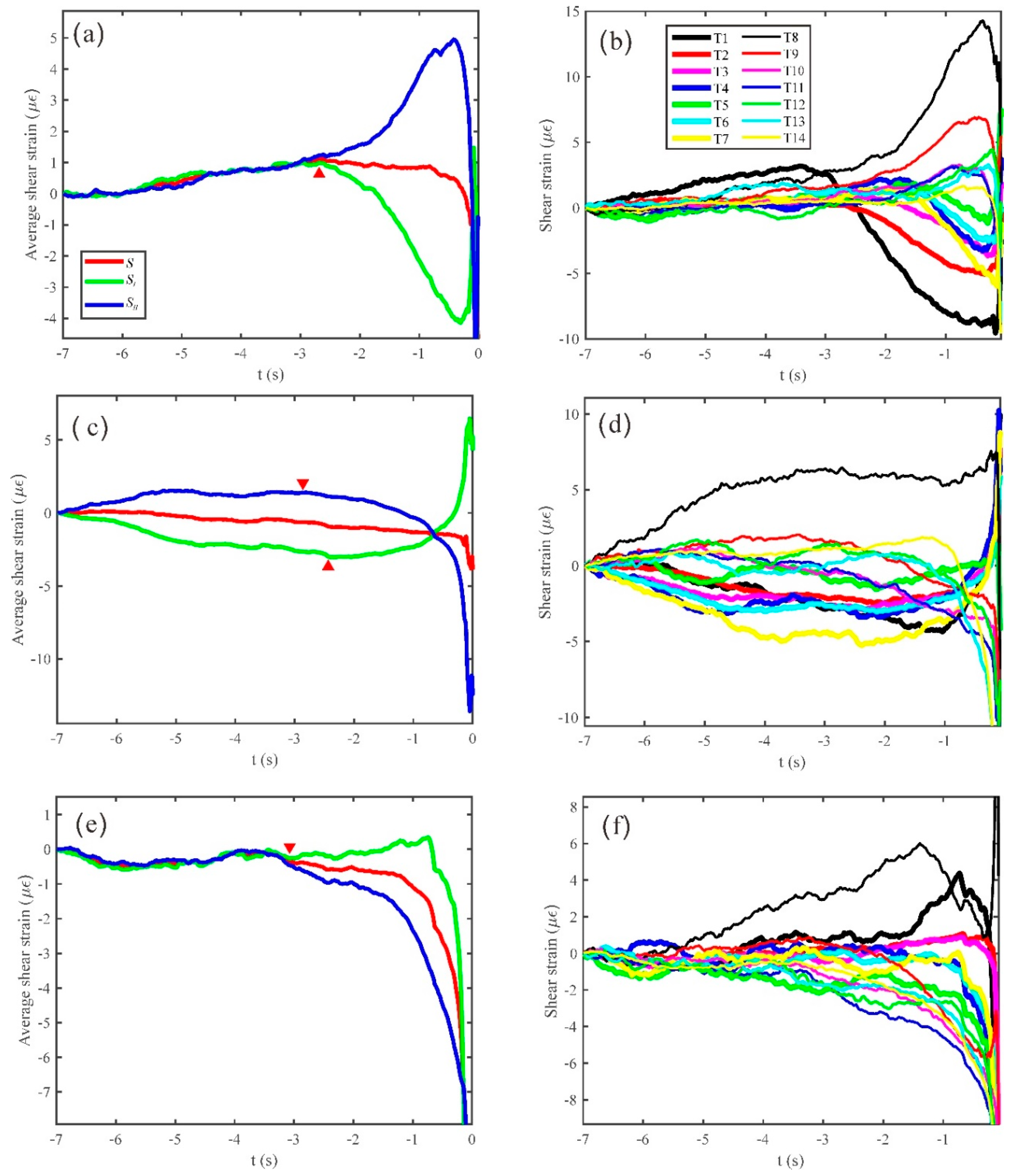
2.3. Strain Gage to Observe Shear Strain along the Fault

An array of 42 resistance strain gages were mounted along the fault on the bottom sample surface, which formed 14 strain gage groups, as shown in Figure 1. The strain gage groups were used to measure the shear strain along the fault and test the results derived from the DIC method. Each strain gage had a resistance grid of 3 × 5 mm with a resistance value of 120.1 ± 0.1 Ω. The sensitivity coefficient of the strain gage was 2.10 ± 1%. Data were acquired by a 96-channel strain acquisition system [21]. The analog-to-digital conversion, sampling rate, and observation error of the device was 16 bit, 100 Hz, and ±1.5 με, respectively. The angles between the three strain gages in each strain gage group and the measured fault segment were 0°, 45°, and 90°. Correspondingly, the offsets of the centers of the three gages from the measured fault segment were 5.0, 12.2, and 6.1 mm, respectively. The plane strain tensor could be obtained by each strain gage group (the specific method was described in previous studies [21,24]), and subsequently, the shear strain of the fault could be calculated.

3. Results

The results obtained from the DIC method show that the rupture process of the bent fault can be divided into two stages: an alternative propagation stage followed by an overall instability stage. The two stages were observed in all three recorded stick-slip events in the experiment.

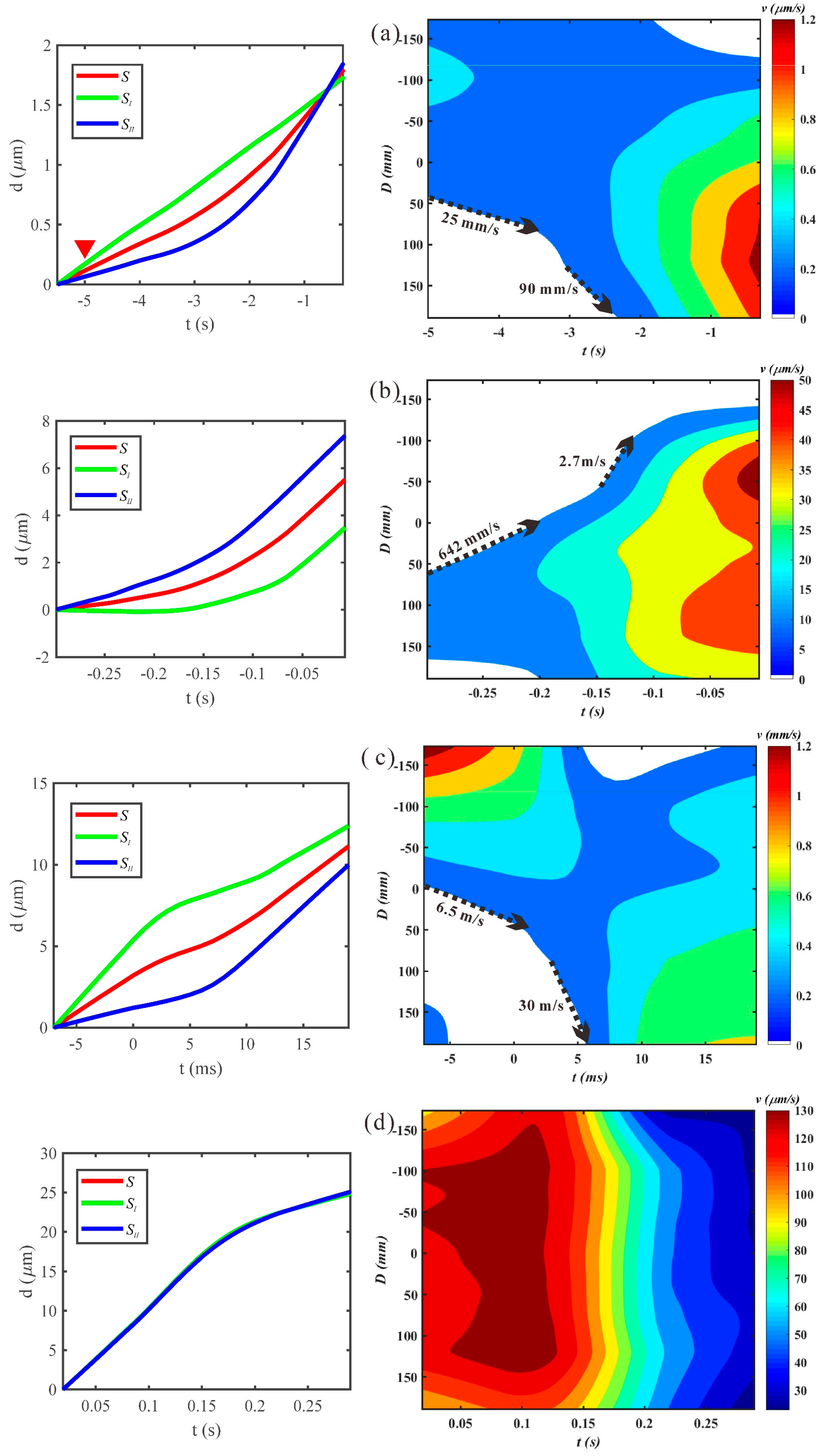
3.1. The Alternative Propagation Stage

The alternative propagation of the rupture between the two fault segments prior to the overall instability of the fault can occur in multiple cycles. During the process, the rupture speed increases from several tens of mm/s to several tens of m/s. Meanwhile, the slip velocity within the rupture also grows from several µm/s to several mm/s. Although the rupture at this stage can propagate between the two fault segments, the rupture speed usually has a jump when the rupture propagates across the fault bend. This indicates the influence of the fault bend on the propagation of the rupture, especially when the slip velocity within the rupture is high as shown in Figure 4b, Figure 5c, and Figure 6b.

Two alternative propagation cycles of the rupture were observed in event E1, as shown in Figure 4. The first cycle began in segment S_I and propagated to segment S_II, as shown in Figure 4a. During this process, the rupture speed accelerated from 16 mm/s in segment S_I to 151 mm/s in segment S_II, and the slip velocity accelerated up to 3 µm/s. The rupture in the second cycle propagated in the opposite direction with respect to that in the first cycle, during which the rupture speed increased from 0.645 m/s in segment S_II to 15 m/s in segment S_I, and the slip velocity increased up to 200 µm/s, as shown in Figure 4b.

Three alternative propagation cycles of the rupture were observed in event E2, as shown in Figure 5. The rupture propagated from segment S_I to segment S_II in the first and the last cycles, as shown in Figure 5a,c, but propagated from segment S_II to segment S_I in the second cycle, as shown in Figure 5b. In the first cycle, only the propagation in the segment S_II was observed. The rupture speed increased from 25 to 90 mm/s and the slip velocity increased up to 1.2 µm/s. During the second cycle, the rupture propagated from segment S_II at a speed of 0.642 m/s to segment S_I at a speed of 2.7 m/s. Meanwhile, the slip velocity increased up to 50 µm/s. In the last cycle, the rupture propagated from segment S_I at a speed of 6.5 m/s to segment S_II at a speed of 30 m/s and the slip velocity increased up to 1200 µm/s.

In event E3, there were also two alternative propagation cycles of the rupture, as shown in Figure 6, which initiated in segment S_II and propagated to segment S_I in the first cycle, as shown in Figure 6a, and propagated in the opposite direction in the second cycle, as shown in Figure 6b. During the first cycle, the rupture speed increased from 142 mm/s in segment S_II to 270 mm/s in segment S_I and the slip velocity accelerated up to 2.5 µm/s. While in the second cycle, the rupture speed increased from 0.128 m/s in segment S_I to 13 m/s in segment S_II and the slip velocity accelerated up to 500 µm/s.

3.2. The Overall Instability Stage

The overall instability stage immediately followed the alternative propagation stage, which was characterized by the almost uniform distribution of slip velocity along the whole fault, as shown in Figure 4c, Figure 5d, and Figure 6c. This indicates that the influence of the fault bend on the rupture propagation was weak in this stage. There were two distinct features at this stage compared with the alternative propagation stage: (1) the slip velocity at this stage was in the order of tens to hundreds of µm/s, as shown in Figure 4c, Figure 5d, and Figure 6c, which was lower than that in the last cycle of the alternative propagation stage, as shown in Figure 4b, Figure 5c, and Figure 6b. (2) The rupture speed in this stage was too high and beyond the observation capability of the high-speed camera due to the sampling rate of 1000 frames per second, and as a result, slip velocity contours were almost perpendicular to the time axis in Figure 4c, Figure 5d, and Figure 6c.

4. Discussion

4.1. Reliability Test of the DIC Method via Strain Gage Measurement

The above fault slip velocity measured by the DIC method spanned a wide range of at least 3 orders of magnitude, as shown in Figure 4, Figure 5, and Figure 6. Although the high slip velocity was easily observed by the DIC method with a high signal-noise ratio, the reliability of the observed low slip velocity needs to be tested, especially in the first cycle of the alternative propagation stage where the slip velocity can be as low as below 1 µm/s, as shown in Figure 4a, Figure 5a, and Figure 6a. Such a low slip velocity leads to a problem of whether the observed velocity was a fault slip or a strain buildup. To make it clear, a high precision measurement of the shear strain along the fault is necessary because local shear strain will drop as local instability occurs in the fault [35,36]. Therefore, we used the evolution of shear strain at the 14 locations along the fault to test whether the observed slip velocity in the first cycle of the alternative propagation stage, as shown in Figure 4a, Figure 5a, and Figure 6a, was a fault slip or a strain buildup. Since the sampling rate of the strain acquisition system was only 100 Hz, the shear strain measurement was unable to test the rupture in other cycles of the alternative propagation stage.

Figure 7 shows the evolution of the shear strain in a duration of 7 s covering the first cycle of the alternative propagation stage of the three stick-slip events. The subgraphs (a) and (b), (c) and (d), (e) and (f) in Figure 7 correspond to events E1, E2, and E3, respectively. The changes of the average shear strain in the whole fault, the segment S_I, and the segment S_II with time are shown on the left side of Figure 7. The changes of the shear strain of each strain gage group with time are shown on the right side of Figure 7. The red triangles in Figure 7a,c,e mark the turning points in the average shear strain of the fault segments. Figure 7a shows that the average shear strain in segment S_I increased and decreased just before and after the red triangle (t ~ −2.8 s), respectively, while the average shear strain continuously increased in segment S_II at the red triangle. These indicate that segment S_I began to slip at t ~ −2.8 s. Figure 7b shows that the rupture initiated near group T1, of which the shear strain dropped first. These are consistent with the results observed in Figure 4a.

The two red triangles in Figure 7c show that the average shear strain in segment S_II changed from ascending to descending at t~−2.8 s, while the average shear strain in segment S_I changed from decreasing to rising at t~−2.4 s. This indicates that the rupture gradually shifted from segment S_I to segment S_II between t~−2.8 s and t~−2.4 s, which is consistent with the evolution of the rupture observed in Figure 5a.

The red triangle in Figure 7e shows that the average shear strain began to rise slowly in segment S_I but decreased in segment S_II after t~−3.1s, indicating that the rupture initiated in segment S_II before it propagated to segment S_I during this period. Figure 7f shows that the shear strain of group T11 dropped first, which indicates that the rupture initiated near group T11. These are consistent with the observations in Figure 6a.

The consistency of the observations between the strain gages and the DIC method indicates that the rupture evolution shown in Figure 4a, Figure 5a, and Figure 6a are reliable.

4.2. The Influences of the Fault Bend on the Rupture Propagation and Further Research

The previous experiments have observed the process of the alternative propagation of the rupture between the two fault segments on both sides of the fault bend [18,19,24]. The process that the rupture initiated at one segment was stopped at the fault bend and restarted after a time delay near the fault bend at another segment prior to the overall instability of the fault [19], which was similar to the last cycle of the alternative propagation stage in our experiment. However, more details of the alternative propagation of the rupture were observed in our experiment, especially the multiple cycles of the alternative propagation process, during which the rupture speed and slip velocity were increasing. This is owing to the high spatial sampling observation of the DIC method.

The boundaries of the slip velocity contours are perpendicular to the time axis in Figure 4c, Figure 5d, and Figure 6c, indicating that the rupture had a rapid propagation speed during the overall instability, which was beyond the recording capability of the high-speed camera with a sampling rate of 1000 frames per second. As a result, the rupture process during the overall instability of the fault could not be fully recorded. Thus, what we can discuss is the alternative propagation stage that was fully recorded. Previous studies have pointed out that the fault bend can serve as an initiation or termination for earthquake ruptures, e.g., [7]. The observed alternative propagation of the rupture in our experiment, as shown in Figure 4, Figure 5 and Figure 6, was also essentially influenced by the fault bend. Namely, the rupture initiated in one fault segment was hindered by the fault bend and accelerated before and after it propagated across the fault bend to another segment, respectively, as shown in Figure 4a,b, Figure 5a–c, and Figure 6a,b. This effect indicates the interaction between the fault bend and the rupture, which is similar to the effect that the asperities hinder and promote the rupture before and after the failure of the asperities in straight faults, respectively [25,35]. On the other hand, unlike straight faults where the failed asperities have been deformed and do not interact with the rupture in the same seismogenic process [25,35], a fault bend is a geometric structure of the fault and is accordingly difficult to be deformed by the rupture. As a result, the fault bend can interact with the rupture in multiple cycles during the same seismogenic process, which was observed in the alternative propagation stage in our experiment.

The process leading to the overall instability of the fault observed in the straight fault is usually accompanied with acceleration in rupture propagation and fault slip, e.g., [26,30,35]. However, this process of the bent fault observed in our experiment is different. Although the rupture accelerated continuously in trend, the slip velocity during the overall instability stage of the bent fault was slower than that in the last cycle of the alternative propagation stage, as shown in Figure 4, Figure 5, and Figure 6. Study of the mechanism of this phenomenon will be very important for further understanding of the conditions for the overall instability of the bent fault. We think that the observation of the detailed spatiotemporal evolution of the rupture propagation during the overall instability of the bent fault may help solve the problem. This depends on the improvement of the temporal sampling rate of the DIC observation system.

5. Conclusions

In this experiment, we used a high-speed camera combined with a DIC method to observe the rupture process of a bent fault with a 5° bending angle between its two segments under biaxial loading, which was also supported by the observation of strain gages. The results show that the evolution of the ruptures was composed of two stages: the alternative propagation between the two fault segments on both sides of the fault bend followed by the overall instability of the fault. Thanks to the dense spatial sampling of the DIC method, multiple alternative propagation cycles of the ruptures between the two fault segments with accelerating rupture speed and slip velocity were found prior to the overall instability of the fault, which indicate the repeated interactions between the ruptures and the fault bend prior to the overall instability of the fault.

References

1. Sangha, S.; Peltzer, G.; Zhang, A.; Meng, L.; Liang, C.; Lundgren, P.; Fielding, E. Fault geometry of 2015, mw7.2 murghab, tajikistan earthquake controls rupture propagation: Insights from insar and seismological data. Earth Planet. Sci. Lett. 2017, 462, 132–141. [Google Scholar] [CrossRef]
2. Elliott, A.J.; Oskin, M.E.; Liu-zeng, J.; Shao, Y.X. Persistent rupture terminations at a restraining bend from slip rates on the eastern altyn tagh fault. Tectonophysics 2018, 733, 57–72. [Google Scholar] [CrossRef]
3. Acharya, H.K. Influence of fault bends on ruptures. Bull. Seismol. Soc. Am. 1997, 87, 1691–1696. [Google Scholar]
4. Barka, A.A.; Kadinsky-Cade, K. Strike-slip fault geometry in turkey and its influence on earthquake activity. Tectonics 1988, 7, 663–684. [Google Scholar] [CrossRef]
5. Ando, R.; Imanishi, K.; Panayotopoulos, Y.; Kobayashi, T. Dynamic rupture propagation on geometrically complex fault with along-strike variation of fault maturity: Insights from the 2014 northern nagano earthquake. Earth Planets Space 2017, 69, 130. [Google Scholar] [CrossRef]
6. Wang, W.-M.; He, Y.-M.; Yao, Z.-X. Complexity of the coseismic rupture for 1999 chi-chi earthquake (Taiwan) from inversion of gps observations. Tectonophysics 2004, 382, 151–172. [Google Scholar] [CrossRef]
7. King, G.; Nábělek, J. Role of fault bends in the initiation and termination of earthquake rupture. Science 1985, 228, 984–987. [Google Scholar] [CrossRef] [PubMed]
8. King, G.C.P. Speculations on the geometry of the initiation and termination processes of earthquake rupture and its relation to morphology and geological structure. Pure Appl. Geophys. 1986, 124, 567–585. [Google Scholar] [CrossRef]
9. Aochi, H.; Fukuyama, E.; Matsu’ura, M. Spontaneous rupture propagation on a non-planar fault in 3-d elastic medium. Pure Appl. Geophys. 2000, 157, 2003–2027. [Google Scholar] [CrossRef]
10. Oglesby, D.D.; Day, S.M. The effect of fault geometry on the 1999 chi-chi (Taiwan) earthquake. Geophys. Res. Lett. 2001, 28, 1831–1834. [Google Scholar] [CrossRef]
11. Duan, B.; Oglesby, D.D. Multicycle dynamics of nonplanar strike-slip faults. J. Geophys. Res. Solid Earth 2005, 110. [Google Scholar] [CrossRef]
12. Kase, Y.; Day, S.M. Spontaneous rupture processes on a bending fault. Geophys. Res. Lett. 2006, 33. [Google Scholar] [CrossRef]
13. Fang, Z.; Xu, G.; Oglesby, D.D. Geometric effects on earthquake nucleation on bent dip-slip faults. Int. J. Appl. Mech. 2011, 3, 99–117. [Google Scholar] [CrossRef]
14. Lozos, J.C.; Oglesby, D.D.; Duan, B.; Wesnousky, S.G. The effects of double fault bends on rupture propagation: A geometrical parameter study. Bull. Seismol. Soc. Am. 2011, 101, 385–398. [Google Scholar] [CrossRef]
15. Zeng, Y.; Chen, C.-H. Fault rupture process of the 20 september 1999 chi-chi, Taiwan, earthquake. Bull. Seismol. Soc. Am. 2001, 91, 1088–1098. [Google Scholar] [CrossRef]
16. Aochi, H.; Fukuyama, E. Three-dimensional nonplanar simulation of the 1992 landers earthquake. J. Geophys. Res. Solid Earth 2002, 107, ESE4-1–ESE4-12. [Google Scholar] [CrossRef]
17. Aochi, H.; Madariaga, R.L. The 1999 Izmit, Turkey, earthquake: Nonplanar fault structure, dynamic rupture process, and strong ground motion. Bull. Seismol. Soc. Am. 2003, 93, 1249–1266. [Google Scholar] [CrossRef]
18. Ma, J.; Ma, W.; Ma, S.; Deng, Z.; Liu, L.; Liu, T. Experimental study and numerical simulation on physical fields during the deformation of a 5° bend fault. Seismol. Geol. 1995, 17, 318–326. [Google Scholar]
19. Kato, N.; Satoh, T.; Lei, X.; Yamamoto, K.; Hirasawa, T. Effect of fault bend on the rupture propagation process of stick-slip. Tectonophysics 1999, 310, 81–99. [Google Scholar] [CrossRef]
20. Rousseau, C.-E.; Rosakis, A.J. On the influence of fault bends on the growth of sub-rayleigh and intersonic dynamic shear ruptures. J. Geophys. Res. Solid Earth 2003, 108. [Google Scholar] [CrossRef]
21. Liu, L.; Ma, J.; Ma, S. Characteristics and evolution of background strain field on typical structure models. Seismol. Geol. 1995, 17, 349–356. [Google Scholar]
22. Ma, J.; Liu, L.; Ma, S. Fault geometry and departure of precursors from the epicenter. Earthq. Res. China 1998, 12, 59–67. [Google Scholar]
23. Guo, Y.-S.; Ma, J.; Yun, L. Experimental study on stick-slip process of bending faults. Seismol. Geol. 2011, 33, 26–35. [Google Scholar]
24. Yun, L.; Guo, Y.-S.; Ma, J. An experimaental study of evolution of physical field and the alternative activities during stick-slip of 5° bend fault. Seismol. Geol. 2011, 33, 356–368. [Google Scholar]
25. Zhuo, Y.-Q.; Liu, P.; Chen, S.; Guo, Y.; Ma, J. Laboratory observations of tremor-like events generated during preslip. Geophys. Res. Lett. 2018, 45, 6926–6934. [Google Scholar] [CrossRef]
26. Zhuo, Y.-Q.; Guo, Y.; Chen, S.; Ji, Y.; Ma, J. Laboratory observations of linkage of preslip zones prior to stick-slip instability. Entropy 2018, 20, 629. [Google Scholar] [CrossRef]
27. Zhuo, Y.-Q.; Bornyakov, S.A.; Guo, Y.-S.; Ma, J.; Sherman, S.I. Influences of obliquity angle difference on the evolution of fen-wei rift: A study from segemented transtension clay model. Seismol. Geol. 2016, 38, 259–277. [Google Scholar]
28. Zhuo, Y.-Q.; Ma, J.; Guo, Y.-S.; Ji, Y.-T. Identification of the meta-instability stage via synergy of fault displacement: An experimental study based on the digital image correlation method. Phys. Chem. Earth Parts A/B/C 2015, 85–86, 216–224. [Google Scholar] [CrossRef]
29. Ji, Y.; Hall, S.A.; Baud, P.; Wong, T.F. Characterization of pore structure and strain localization in majella limestone by x-ray computed tomography and digital image correlation. Geophys. J. Int. 2015, 200, 699–717. [Google Scholar] [CrossRef]
30. Zhuo, Y.; Guo, Y.; Ji, Y.; Ma, J. Slip synergism of planar strike-slip fault during meta-instable state: Experimental research based on digital image correlation analysis. Sci. China Earth Sci. 2013, 56, 1881–1887. [Google Scholar] [CrossRef]
31. Rudnick, R.L.; Gao, S. 3.01—Composition of the continental crust. In Treatise on Geochemistry; Holland, H.D., Turekian, K.K., Eds.; Pergamon: Oxford, UK, 2003; pp. 1–64. [Google Scholar]
32. Sutton, M.A.; Wolters, W.J.; Peters, W.H.; Ranson, W.F.; McNeill, S.R. Determination of displacements using an improved digital correlation method. Image Vis. Comput. 1983, 1, 133–139. [Google Scholar] [CrossRef]
33. Peters, W.H.; Ranson, W.F. Digital imaging techniques in experimental stress analysis. OPTICE 1982, 21, 213427. [Google Scholar] [CrossRef]
34. Yamaguchi, I. A laser-speckle strain gauge. J. Phys. E Sci. Instrum. 1981, 14, 1270–1273. [Google Scholar] [CrossRef]
35. McLaskey, G.C.; Kilgore, B.D. Foreshocks during the nucleation of stick-slip instability. J. Geophys. Res. Solid Earth 2013, 118, 2982–2997. [Google Scholar] [CrossRef]
36. Dieterich, J.H. Preseismic fault slip and earthquake prediction. J. Geophys. Res. 1978, 83, 3940. [Google Scholar] [CrossRef]
Figure 1. Experimental design. The field of view of the high-speed camera covers the entire sample surface. The D-axis coincides with the fault trace. The common origins of the D-, X-, and Y-axis coincide with the bend point of the fault. The fault is divided into segments SI and SII. The red lines on both sides of the fault are each composed of 1700 measuring points (pixels), which are symmetric with the fault and offset 5.839 mm from the fault. T1–T14 are the numbers of 14 strain gage groups mounted along the fault on the bottom sample surface. The inset pointing to the T5 strain gage group shows details of the arrangement of the three strain gages forming the strain gage group on the sample surface. The illustration on the right is an enlarged view of the fault slip gages in the dashed circle around the fault bend. The red solid circles are the measuring points (pixels) with a 5.839 mm offset from the fault. The green and blue dashed lines connecting the measuring points (corresponding to segments SI and SII, respectively) are auxiliary lines, indicating that the two connected measuring points are symmetrically distributed with respect to the fault and form a fault slip gage. The spacing of the fault slip gages in the same fault segment is 0.214 mm.
Applsci 09 00933 g001
Figure 2. Variations of the differential stress (σ1-σ2) and piston displacement along the Y-axis (dy) with time (t). The inset is a magnified view of the black rectangular zone showing details of the stress drops during a loading rate of 0.5 µm/s. E1, E2, and E3 are the numbers of the stick-slip events indicated by the arrows, which are also the events observed by the high-speed camera.
Applsci 09 00933 g002
Figure 3. Influence of the side length of the subregion (R) on the correlation coefficient (CC) during the calculation of the DIC method. Crosses denote the mean value of 1–CC, error bars indicate the standard deviations, and the cross and error bar in red correspond to the optimal subregion side length.
Applsci 09 00933 g003
Figure 4. Spatiotemporal distribution of fault slips and slip velocity before and after the overall instability of event E1. The subgraphs on the left side show the change of the average slip of the whole fault (S), the segment SI (SI), and the segment SII (SII) with time. D = 0, D < 0, and D > 0 denote the fault bend point, the segment SI, and the segment SII, respectively. The subgraphs on the right side show the spatiotemporal distribution of the fault slip velocity (v). The black dotted arrows and numbers represent the directions and propagation speeds of ruptures, respectively. Note that the time span of the left subgraph is larger than that of the right subgraph in (a). The red triangle in the left subgraph in (a) denotes the beginning of the obvious slip velocity that can be observed; spatiotemporal evolution of slip velocity after which is shown in the right subgraph in (a). The time spans of the left and right subgraphs in (b,c) are consistent. The time axes from (a) to (c) are continuous. The common timing point of the data from the DIC method and strain gages is set zero for each stick-slip event. Accordingly, time before and after the common timing point is negative and positive, respectively.
Applsci 09 00933 g004
Figure 5. Spatiotemporal distribution of fault slips and slip velocity before and after the overall instability of event E2. The time spans of the left and right subgraphs in (bd) are consistent. The time axes from (a) to (d) are continuous. Other labels are the same as shown in Figure 4.
Applsci 09 00933 g005
Figure 6. Spatiotemporal distribution of fault slips and slip velocity before and after the overall instability of event E3. The time axes from (a) to (c) are continuous. Labels are the same as shown in Figure 4.
Applsci 09 00933 g006
Figure 7. Variations of the shear strain with time. (af) correspond to events E1, E2, and E3, respectively. (a,c,e) are the average shear strains in the whole fault (S), the segment SI (SI), and the segment SII (SII), respectively. The red triangles indicate the turning points in the trend of the average shear strain. (b,d,f) are the shear strains in each strain gage group. Groups T1–T7, which are mounted in the segment SI, are displayed with thick lines. Groups T8–T14, which are mounted in the segment SII, are displayed with thin lines. The common timing point of the data from the DIC method and strain gages is set zero for each stick-slip event. Accordingly, the time before and after the common timing point is negative and positive, respectively.
Applsci 09 00933 g007