Prediction Model for the Anisotropic Thermal Conductivity of a 2.5-D Braided Ceramic Matrix Composite with Thin-Wall Structure

Abstract
:1. Introduction
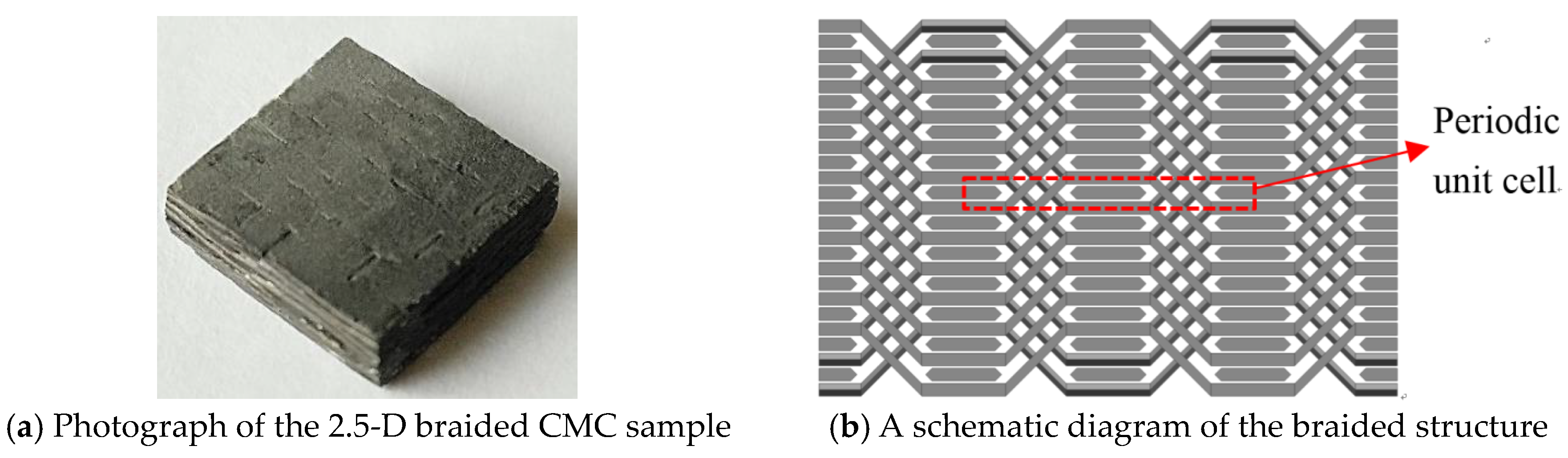
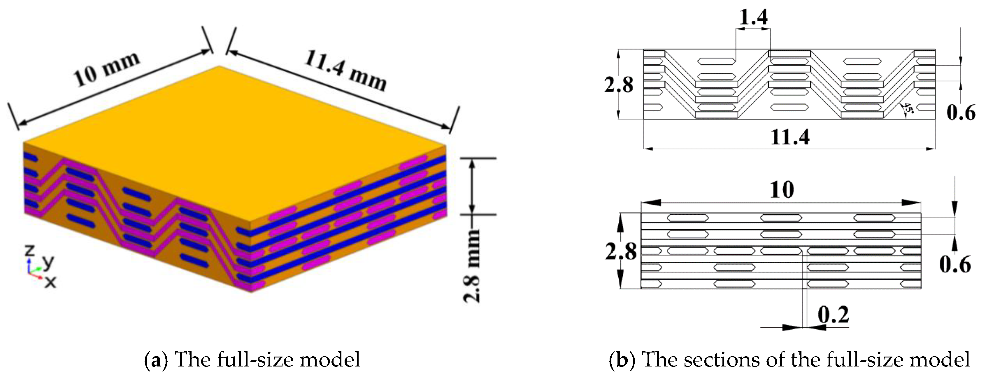
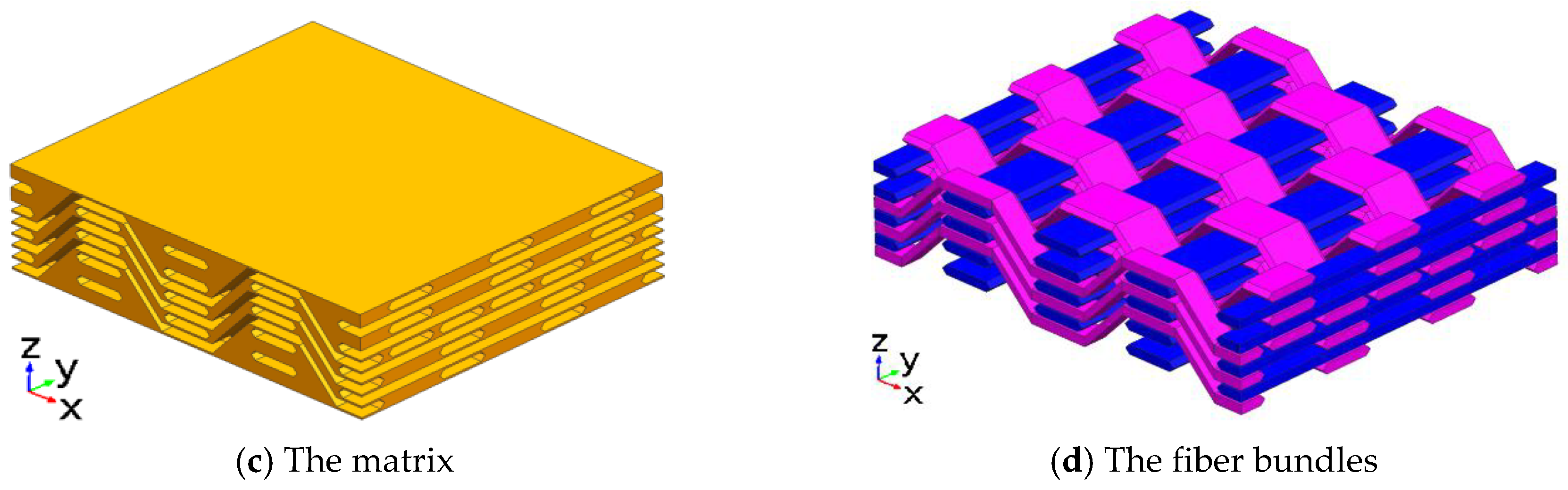
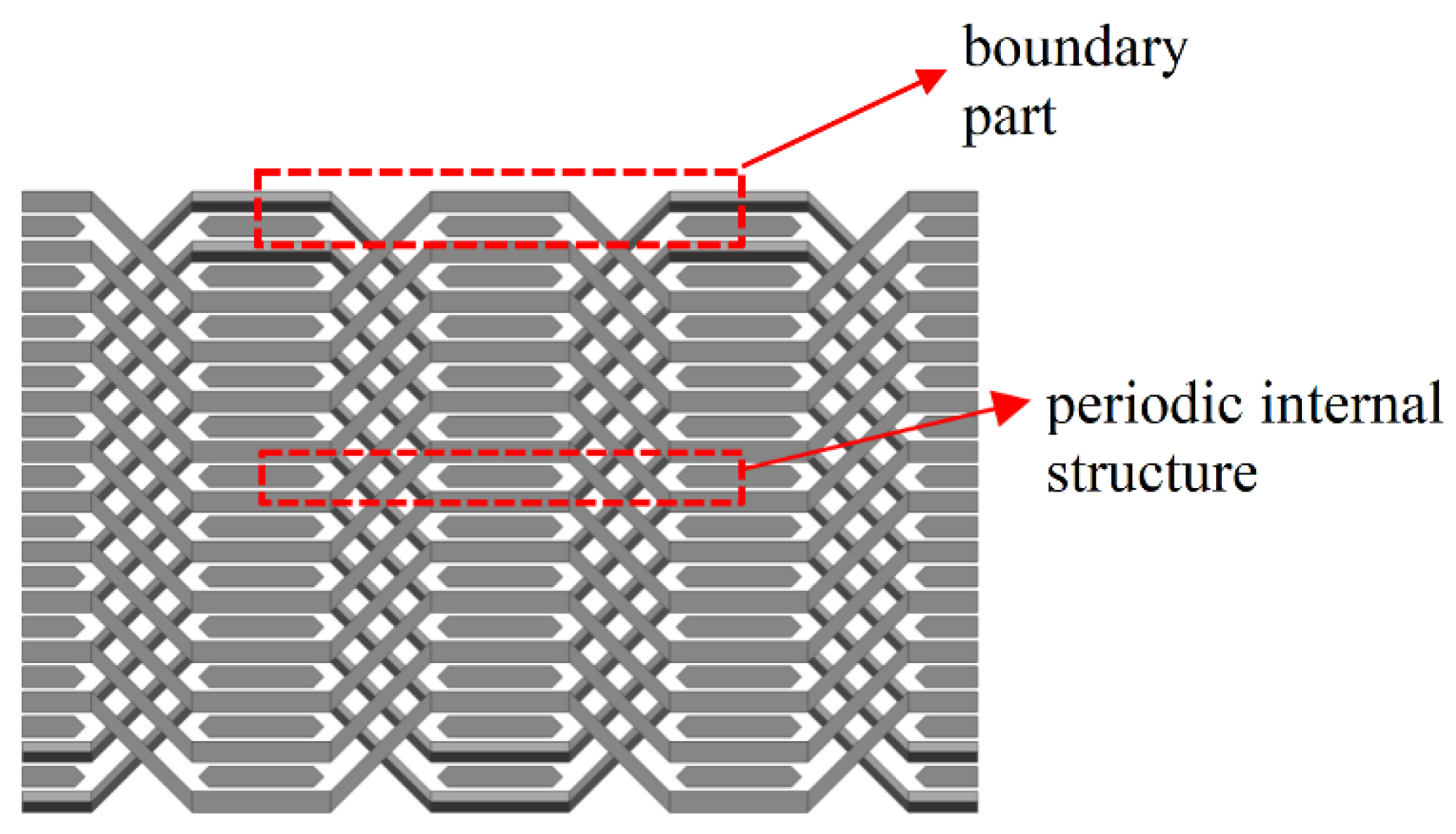
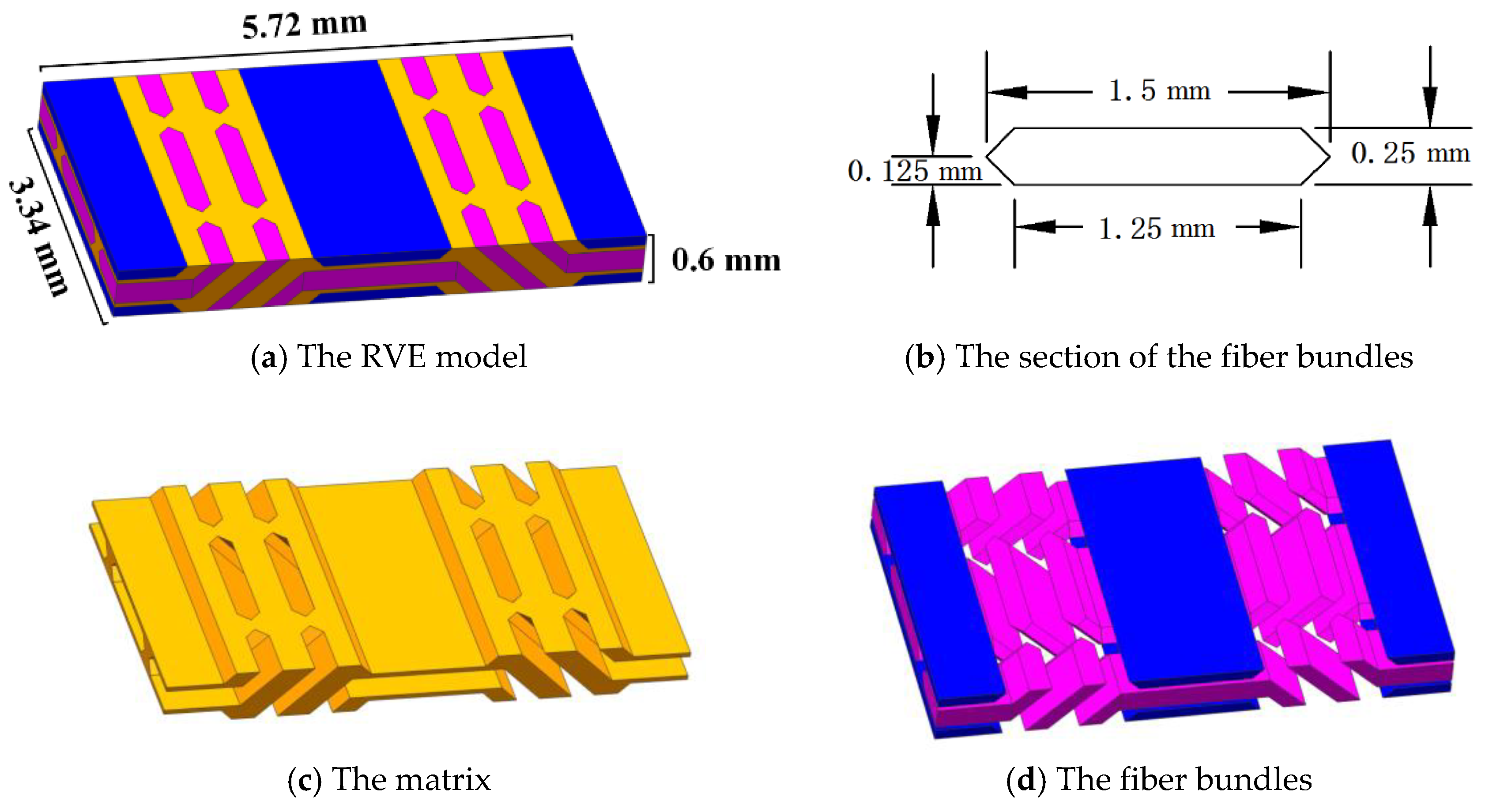
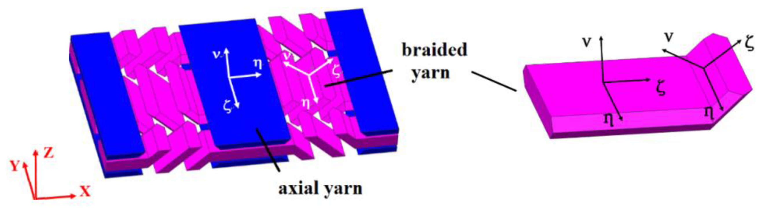
2. Research Models
- The sections of the axial yarns and the braided yarns are both hexagons.
- There are no cracks in the models. Instead, they are completely continuous.
3. Numerical Methodology
3.1. Governing Equations
3.2. Application of the ATC
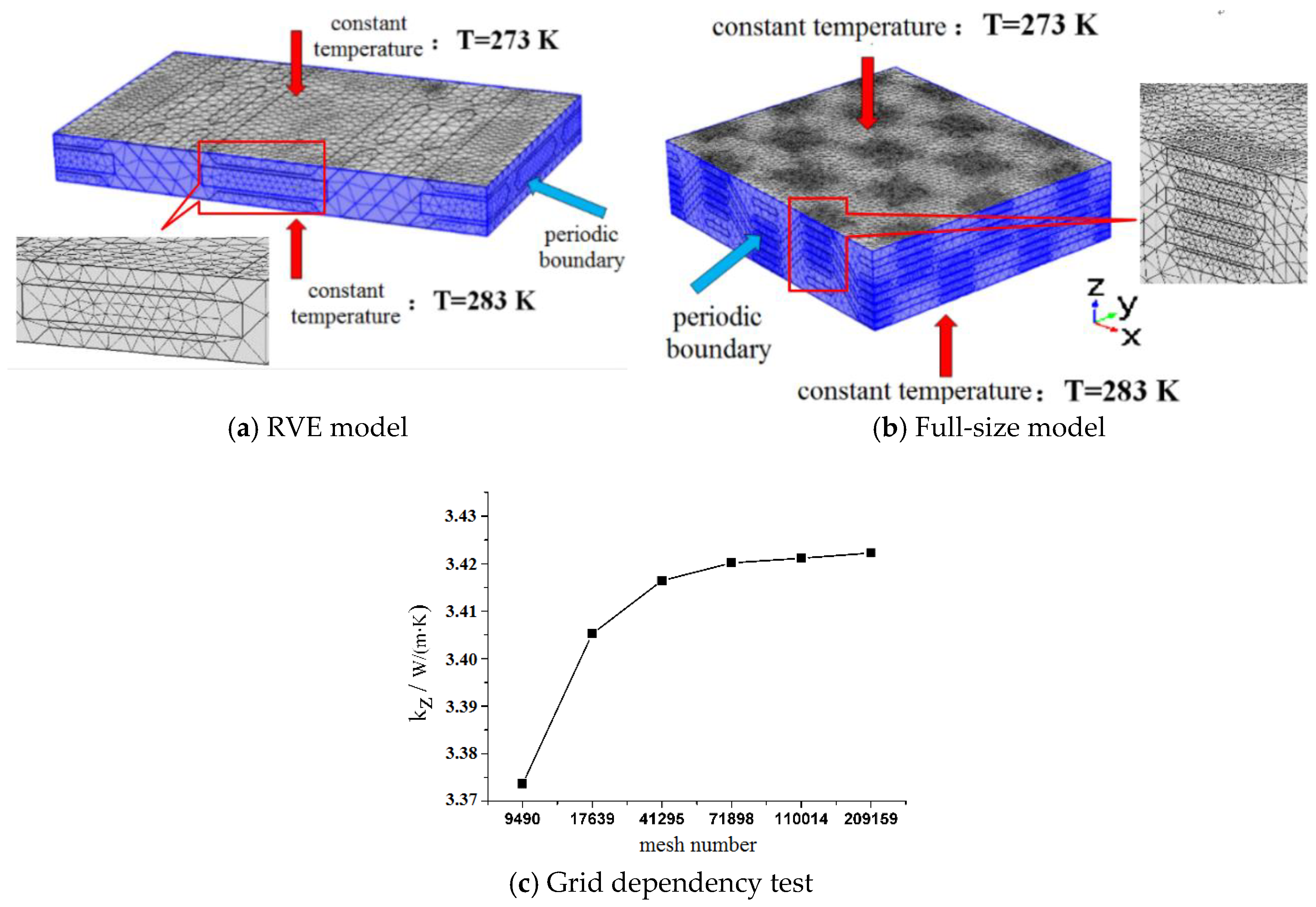
3.3. Mesh and Boundary Conditions
3.4. Operating Conditions and Parameters Definition
4. Results and Discussions
4.1. Comparison between the RVE Model and the Full-Size Model
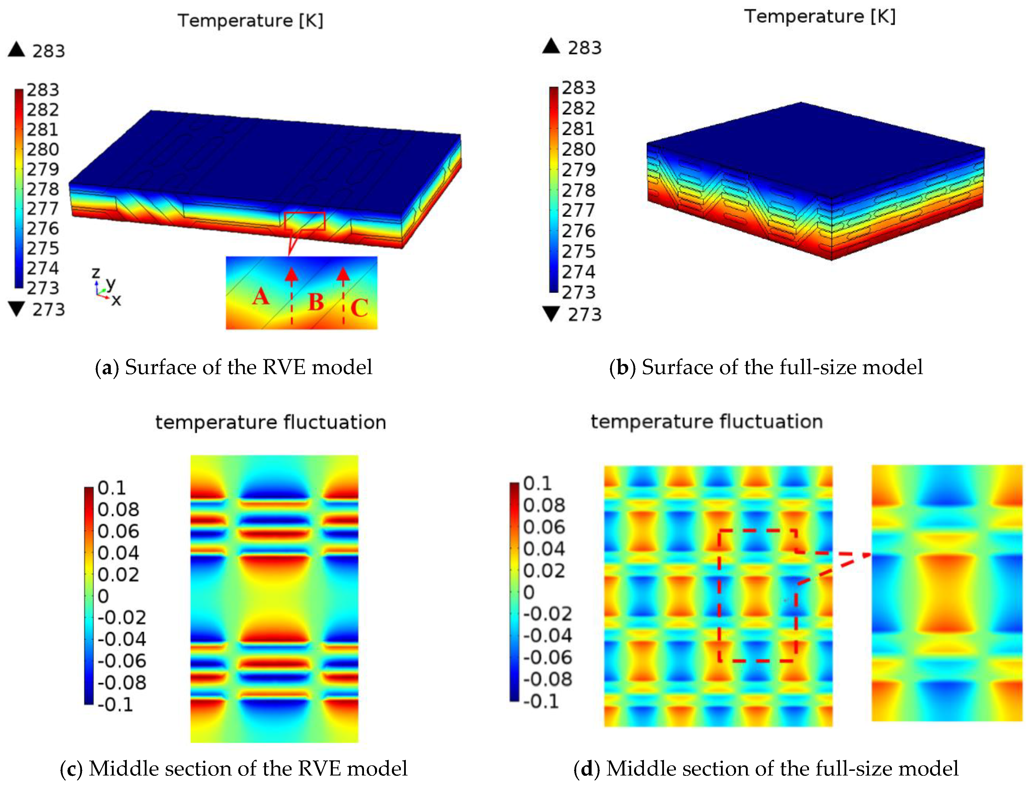
4.1.1. Temperature Field
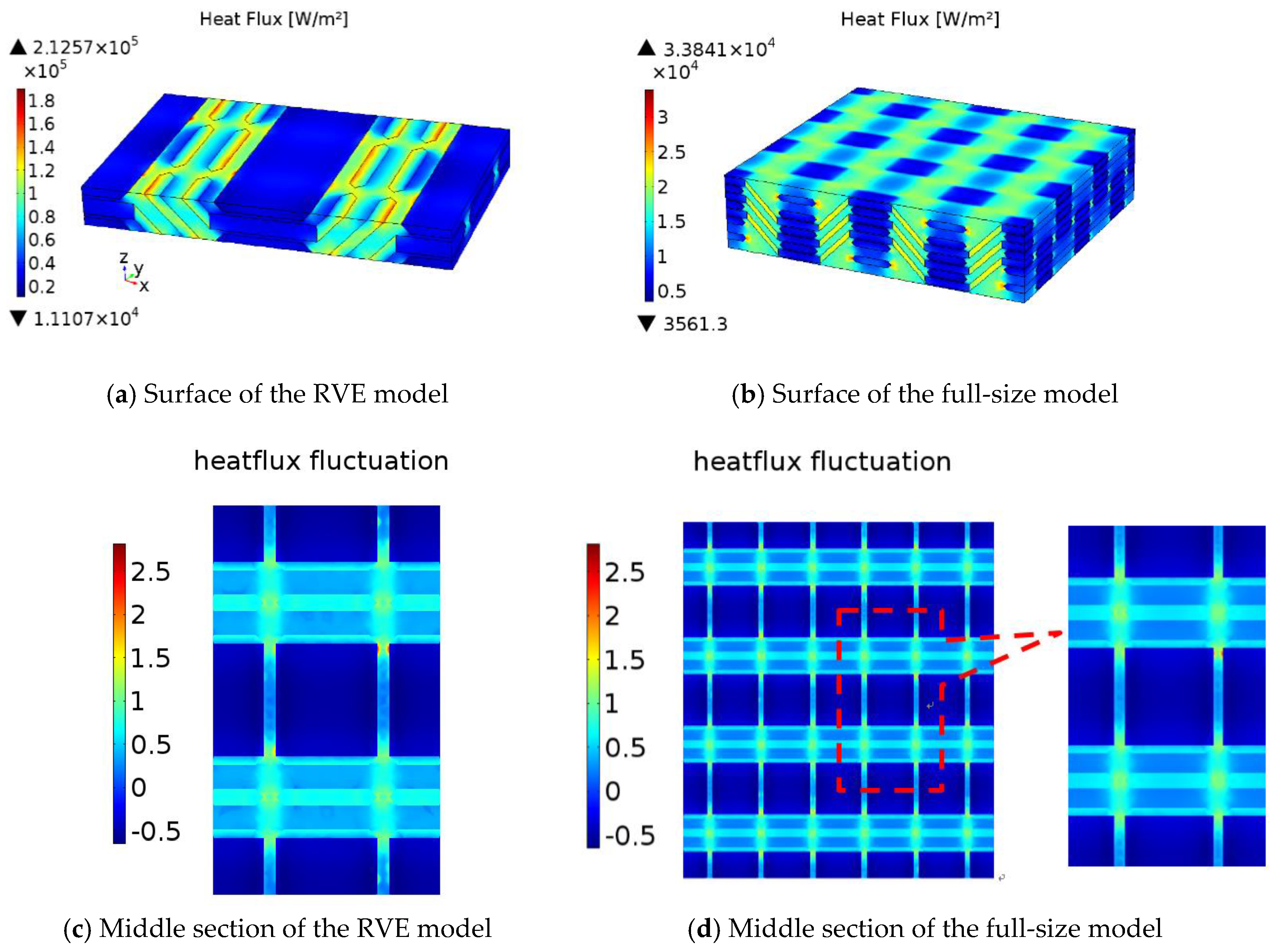
4.1.2. Heat Flux Field
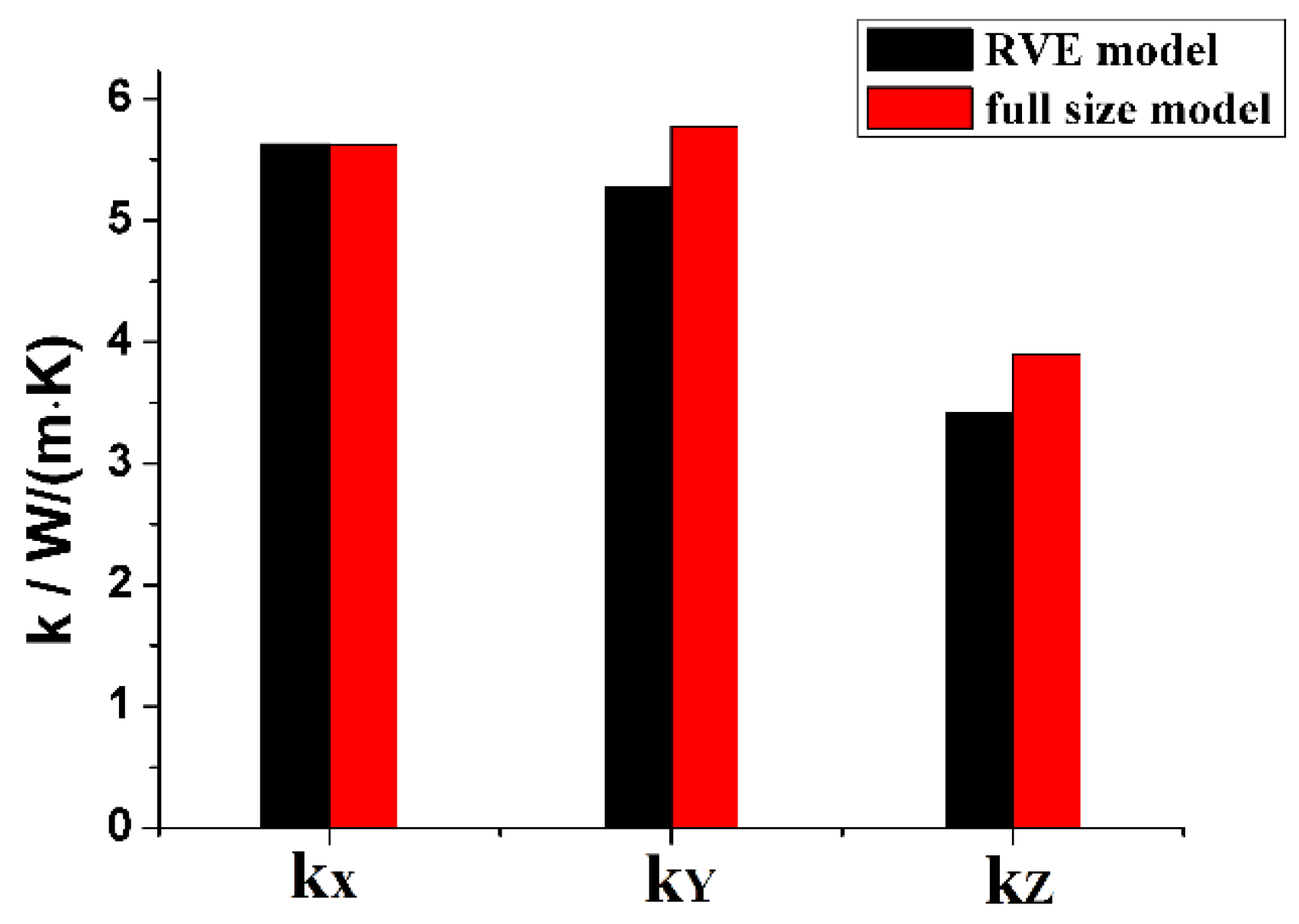
4.1.3. Effective Thermal Conductivity
4.1.4. Validation of the RVE Model and the Full-Size Model
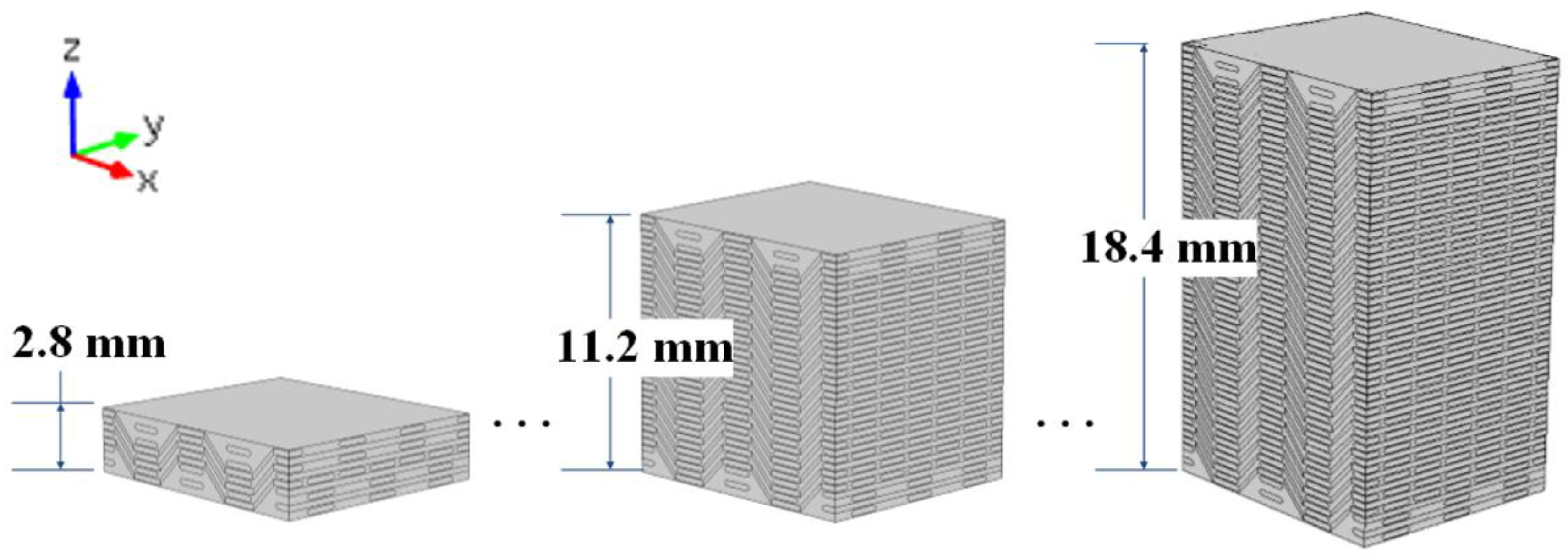
4.2. Influence of the Thickness
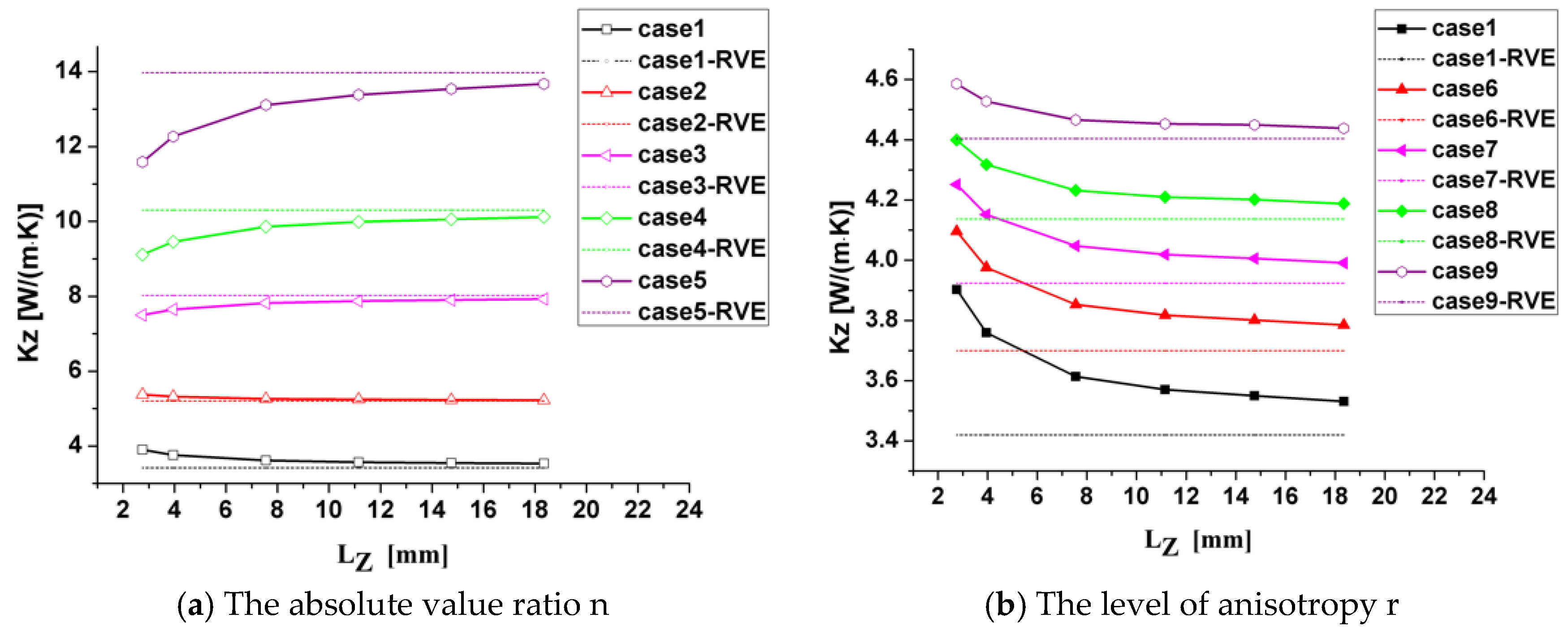
4.3. Results with Different ATCs
5. Conclusions
- (1)
- The temperature field and the heat flux field inside the 2.5-D braided CMC material were clearly heterogeneous, and these fields were affected by the difference between the thermal conductivities of the fiber bundles and matrix. For example, in the full-size model, the relative fluctuation of the temperature field and the relative fluctuation of the heat flux field in the middle section reached 6.39% and 280.40%, respectively.
- (2)
- In the thermal analysis of a thin-walled structure, such as a turbine vane, the RVE model would lead to a large deviation in the estimation of the effective thermal conductivity so that the periodic hypothesis could not be satisfied. The relative variation of the thermal conductivity based on the RVE model compared with the experimental data was 15.62%, while the relative variation was only 3.53% when the full-size model was applied.
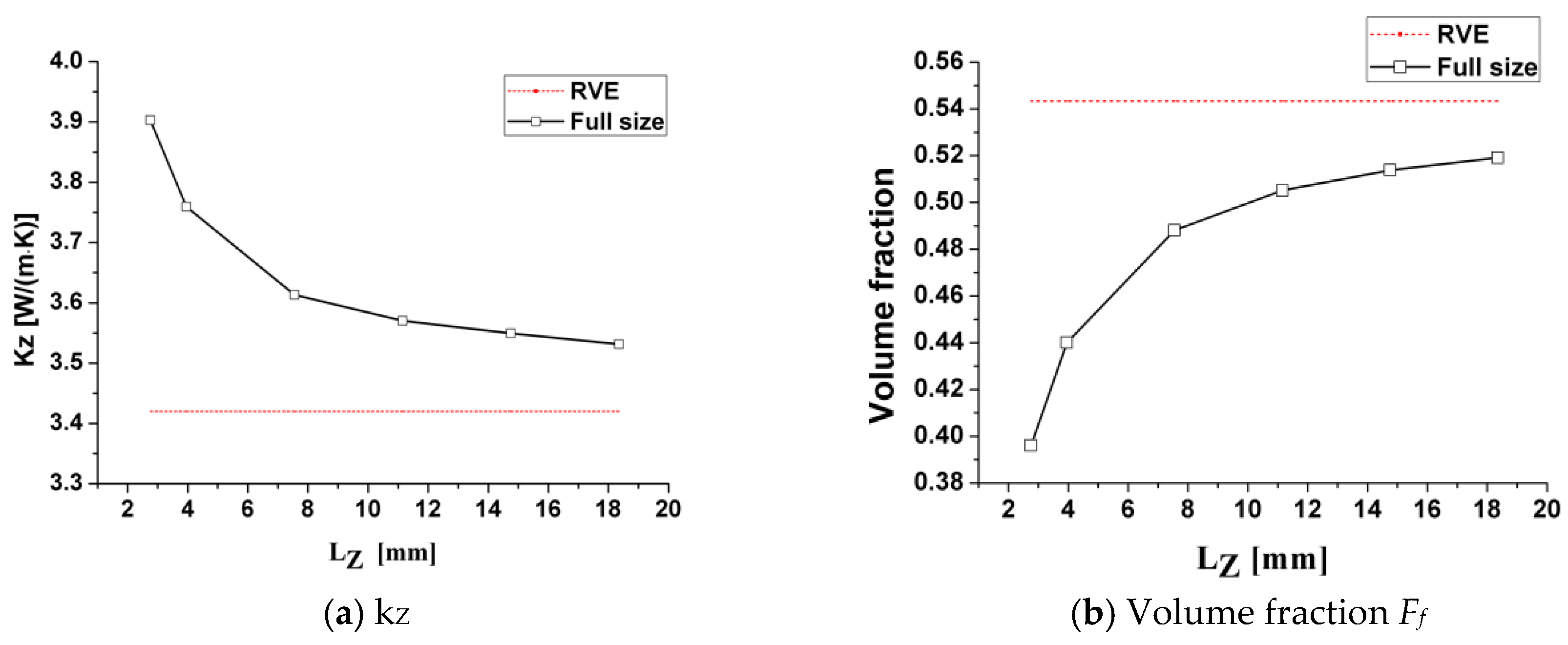
- (3)
- When the thickness increased, the effective thermal conductivities based on the RVE model and the full-size model were close to each other. For the ATC of the sample used in this study, when the thickness was bigger than the critical thickness of 18.4 mm, the RVE model was suitable for the prediction of the ATC.
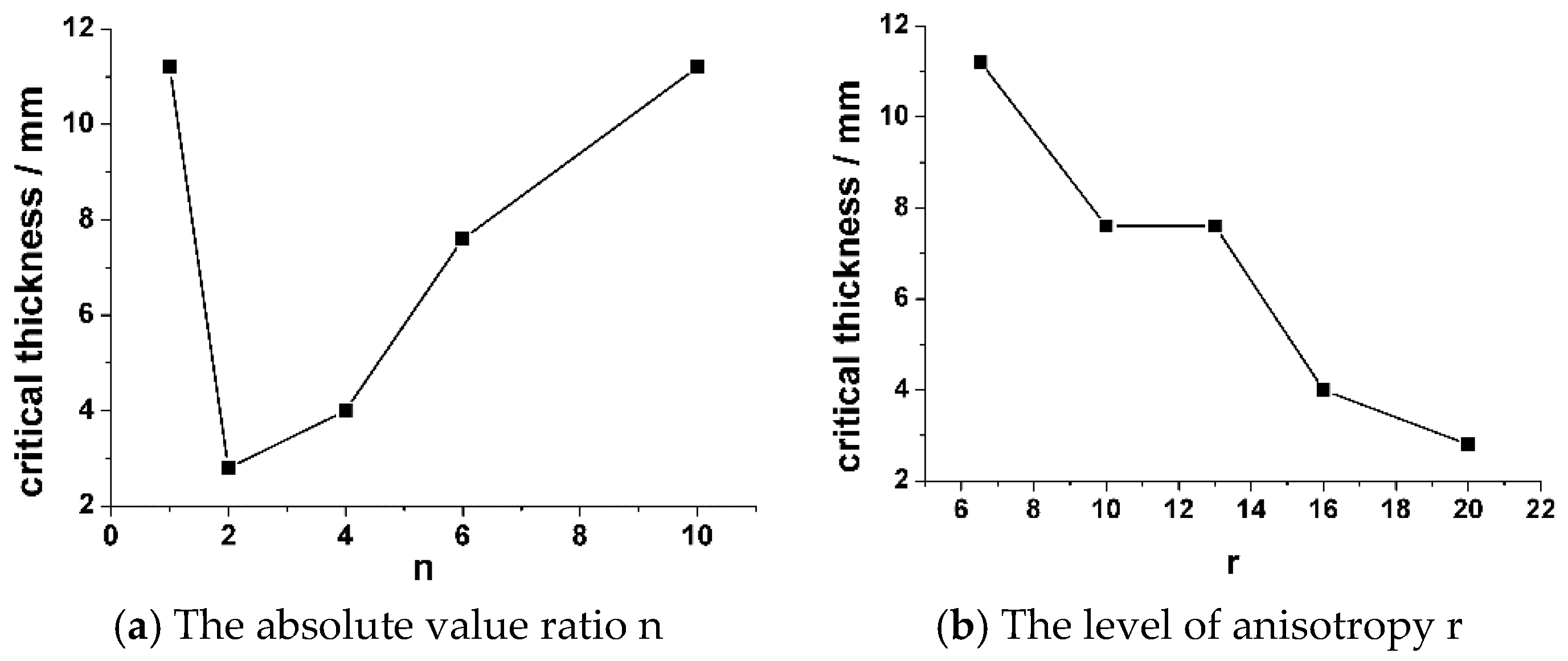
- (4)
- When the absolute value ratio and the level of anisotropy of the thermal conductivities of the fiber bundle were changed, the influence of the thickness on the thermal conductivity was different and the critical thickness for the RVE model changed. When the absolute value ratio increased, the critical thickness firstly decreased and then increased, and the critical thickness decreased almost monotonously with increasing the level of anisotropy.
Author Contributions
Funding
Acknowledgments
Conflicts of Interest
Nomenclature
| Cp | Specific heat capacity at constant pressure (J/(kg·K)) |
| F | Volume fraction |
| k | Thermal conductivity (W/(m·K)) |
| L | Thickness (mm) |
| n | Absolute value ratio comparing to the sample’s ATC |
| r | Anisotropy’s level |
| T | Temperature (K) |
| Velocity (m/s) | |
| X, Y, Z | Global Cartesian coordinates |
| Greek symbols | |
| α | Rotation angles around the x-axis between the PDTC coordinates and the global coordinates (°) |
| β | Rotation angles around the y-axis between the PDTC coordinates and the global coordinates (°) |
| γ | Rotation angles around the z-axis between the PDTC coordinates and the global coordinates (°) |
| ρ | Density (kg/m3) |
| ζ, η, ν | Local Cartesian coordinates |
| δ | Relative fluctuation |
| Subscripts | |
| f | Fiber |
| ij | Coordinates of the mesh nodes |
Abbreviations
| ATC | Anisotropic Thermal Conductivity |
| CMC | Ceramic Matrix Composite |
| ETC | Effective Thermal Conductivity |
| FEM | Finite Element Method |
| PDTC | Principal Direction of Thermal Conductivity |
| RVE | Representative Volume Element |
References
- Fang, C.D. Development Research of Aeroengine; Aviation Industry Press: Beijing, China, 2009. [Google Scholar]
- Hiroshi, K. The application of ceramic-matrix composites to the automotive ceramic gas turbine. Compos. Sci. Technol. 1999, 59, 861–872. [Google Scholar]
- Deng, Y.; Li, W.G.; Wang, R.Z. The temperature-dependent fracture models for fiber-reinforced ceramic matrix composites. Compos. Struct. 2016, 140, 534–539. [Google Scholar] [CrossRef]
- Yang, J.S.; Dong, S.M.; Xu, C.Y. Mechanical response and microstructure of 2D carbon fiber reinforced ceramic matrix composites with SiC and Ti3SiC2 fillers. Ceram. Int. 2016, 42, 3019–3027. [Google Scholar] [CrossRef]
- Michael, V.; Anthony, C.; Robinson, R.C.; Thomas, D.J. Ceramic Matrix Composite Vane Subelement Testing in a Gas Turbine Environment; ASME: New York, NY, USA, 2004. [Google Scholar]
- Heidmann, J.D.; Kassab, A.J.; Divo, E.A.; Rodriguez, F.; Steinthorsson, E. Conjugate Heat Transfer Effects on a Realistic Film-Cooled Turbine Vane; ASME: New York, NY, USA, 2003. [Google Scholar]
- Behzad, T.; Sain, M. Measurement and prediction of thermal conductivity for hemp fiber reinforced composites. Polym. Eng. Sci. 2007, 10, 977–983. [Google Scholar] [CrossRef]
- Xu, Y.B.; Yagi, K. Automatic FEM model generation for evaluating thermal conductivity of composite with random materials arrangement. Comput. Mater. Sci. 2004, 30, 242–250. [Google Scholar] [CrossRef]
- Lebel, L.; Turenne, S.; Boukhili, R. An experimental apparatus and procedure for the simulation of thermal stresses in gas turbine combustion chamber panels made of ceramic matrix composites. J. Eng. Gas Turbines Power 2017, 139, 091502. [Google Scholar] [CrossRef]
- Tu, Z.C.; Mao, J.K.; Jiang, H.; Han, X.; He, Z. Numerical method for the thermal analysis of a ceramic matrix composite turbine vane considering the spatial variation of the anisotropic thermal conductivity. Appl. Therm. Eng. 2017, 127, 436–452. [Google Scholar] [CrossRef]
- Xin, L.I.U.; Xiuli, S.H.E.N.; Longdong, G.O.N.G.; Peng, L.I. Multi-scale thermodynamic analysis method for 2D SiC/SiC composite turbine guide vanes. Chin. J. Aeronaut. 2018, 31, 117–125. [Google Scholar]
- Kiani, S.; Chan, W.S.; Sheikh, A.H. Measurement of thermal conductivity of triaxial braided composites. J. Compos. Mater. 2008, 42, 12. [Google Scholar] [CrossRef]
- Jiang, L.L.; Xu, G.D.; Cheng, S. Predicting the thermal conductivity and temperature distribution in 3D braided composites. Compos. Struct. 2014, 108, 578–583. [Google Scholar] [CrossRef]
- Dasgupta, A.; Agarwal, R.K. Orthotropic thermal conductivity of plain-weave fabric composites using a homogenization technique. J. Compos. Mater. 1992, 26, 2736–2758. [Google Scholar] [CrossRef]
- Ning, Q.G.; Chou, T.W. Closed-form solutions of the in-plane effective thermal conductivities of woven-fabric composites. Compos. Sci. Technol. 1995, 55, 41–48. [Google Scholar] [CrossRef]
- Bhattacharjee, D.; Kothari, V.K. A theoretical model to predict the thermal resistance of plain woven fabrics. Indian J. Fibre Text. Res. 2005, 30, 252–257. [Google Scholar]
- Hill, R. Elastic properties of reinforced solids: Some theoretical principles. J. Mech. Phys. Solids 1963, 11, 357–372. [Google Scholar] [CrossRef]
- Siddiqui, M.O.R.; Sun, D.M. Finite element analysis of thermal conductivity and thermal resistance behavior of woven fabric. Comput. Mater. Sci. 2013, 75, 45–51. [Google Scholar] [CrossRef]
- Ai, S.G.; He, R.J.; Pei, Y.M. A numerical study on the thermal conductivity of 3D woven C/C composites at high temperature. Appl. Compos. Mater. 2015, 22, 823–835. [Google Scholar]
- Fang, W.Z.; Chen, L.; Gou, J.J.; Tao, W.Q. Predictions of effective thermal conductivities for three-dimensional four-directional braided composite using the lattice Boltzmann method. Int. J. Heat Mass Transfer 2016, 92, 120–130. [Google Scholar] [CrossRef]
- Islam, M.R.; Pramila, A. Thermal conductivity of fiber reinforced composites by FEM. J. Compos. Mater. 1999, 33, 1699–1715. [Google Scholar] [CrossRef]
- Klett, J.W.; Ervin, V.J.; Edie, D.D. Finite-element modeling of heat transfer in carbon/carbon composites. Compos. Sci. Technol. 1999, 59, 593–607. [Google Scholar] [CrossRef]
- Car, E.; Zalamea, F.; Oller, S.; Miquel, J.; Qnate, E. Numerical simulation of composite materials: Two procedures. Int. J. Solid Struct. 2002, 39, 1967–1986. [Google Scholar] [CrossRef]
- Dong, K.; Liu, K.; Pan, L.J.; Gu, B.H.; Sun, B.Z. Experimental and numerical investigation on the thermal conduction properties of 2.5D angle-interlock woven composites. Compos. Struct. 2016, 154, 319–333. [Google Scholar] [CrossRef]
- Guan, T.R. Micro Geometry and Mechanical Model and Experimental Study of 2.5D Braided Quartz/SiO2 Ceramic Matrix Composites; Nanjing University of Aeronautics and Astronautics: Nanjing, China, 2012. [Google Scholar]
- COMSOL. COMSOL Multiphysics Help—Theory for the Heat Transfer, Release 4.3, Sweden. 2011. [Google Scholar]
- Ree, Y.; Lin, J.R.; Zhu, J.G. Coordinate transformation uncertainty analysis in Larger-Scale metrology. IEEE Trans. Instrum. Meas. 2015, 64, 2380–2388. [Google Scholar]
- He, F. Carbon Fiber and Graphite Fiber; Chemical Industry Press: Beijing, China, 2010. [Google Scholar]


| Case | kζ/kη/kν W/(m·K) | n | r |
|---|---|---|---|
| 1 | 9.66/1.48/1.48 | 1 | 6.53 |
| 2 | 19.32/2.96/2.96 | 2 | 6.53 |
| 3 | 38.64/5.92/5.92 | 4 | 6.53 |
| 4 | 57.96/8.88/8.88 | 6 | 6.53 |
| 5 | 96.6/14.8/14.8 | 10 | 6.53 |
| 6 | 14.8/1.48/1.48 | / | 10 |
| 7 | 19.24/1.48/1.48 | / | 13 |
| 8 | 23.68/1.48/1.48 | / | 16 |
| 9 | 29.6/1.48/1.48 | / | 20 |
| Experimental Data | Numerical Data | ||||||||||
|---|---|---|---|---|---|---|---|---|---|---|---|
| Thermal Diffusivity/m2/s | Thermal Conductivity kZ/W/(m·K) | Mean Value/W/(m·K) | Standard Deviation/W/(m·K) | RVE Model/W/(m·K) | Full-Size Model/W/(m·K) | ||||||
| 3.427 | 3.460 | 3.444 | 3.443 | 4.036 | 4.072 | 4.053 | 4.052 | 4.053 | 0.015 | 3.42 | 3.91 |
© 2019 by the authors. Licensee MDPI, Basel, Switzerland. This article is an open access article distributed under the terms and conditions of the Creative Commons Attribution (CC BY) license (http://creativecommons.org/licenses/by/4.0/).
Share and Cite
Tu, Z.; Mao, J.; Han, X.; He, Z. Prediction Model for the Anisotropic Thermal Conductivity of a 2.5-D Braided Ceramic Matrix Composite with Thin-Wall Structure. Appl. Sci. 2019, 9, 875. https://doi.org/10.3390/app9050875
Tu Z, Mao J, Han X, He Z. Prediction Model for the Anisotropic Thermal Conductivity of a 2.5-D Braided Ceramic Matrix Composite with Thin-Wall Structure. Applied Sciences. 2019; 9(5):875. https://doi.org/10.3390/app9050875
Chicago/Turabian StyleTu, Zecan, Junkui Mao, Xingsi Han, and Zhenzong He. 2019. "Prediction Model for the Anisotropic Thermal Conductivity of a 2.5-D Braided Ceramic Matrix Composite with Thin-Wall Structure" Applied Sciences 9, no. 5: 875. https://doi.org/10.3390/app9050875
APA StyleTu, Z., Mao, J., Han, X., & He, Z. (2019). Prediction Model for the Anisotropic Thermal Conductivity of a 2.5-D Braided Ceramic Matrix Composite with Thin-Wall Structure. Applied Sciences, 9(5), 875. https://doi.org/10.3390/app9050875