Selection of Optimal Hyperspectral Wavebands for Detection of Discolored, Diseased Rice Seeds

Abstract

The inspection of rice grain that may be infected by seedborne disease is important for ensuring uniform plant stands in production fields as well as preventing proliferation of some seedborne diseases. The goal of this study was to use a hyperspectral imaging (HSI) technique to find optimal wavelengths and develop a model for detecting discolored, diseased rice seed infected by bacterial panicle blight (Burkholderia glumae), a seedborne pathogen. For this purpose, the HSI data spanning the visible/near-infrared wavelength region between 400 and 1000 nm were collected for 500 sound and discolored rice seeds. For selecting optimal wavelengths to use for detecting diseased seed, a sequential forward selection (SFS) method combined with various spectral pretreatments was employed. To evaluate performance based on optimal wavelengths, support vector machine (SVM) and linear and quadratic discriminant analysis (LDA and QDA) models were developed for detection of discolored seeds. As a result, the violet and red regions of the visible spectrum were selected as key wavelengths reflecting the characteristics of the discolored rice seeds. When using only two or only three selected wavelengths, all of the classification methods achieved high classification accuracies over 90% for both the calibration and validation sample sets. The results of the study showed that only two to three wavelengths are needed to differentiate between discolored, diseased and sound rice, instead of using the entire HSI wavelength regions. This demonstrates the feasibility of developing a low cost multispectral imaging technology based on these selected wavelengths for non-destructive and high-throughput screening of diseased rice seed.

1. Introduction

Rice seeds are known to harbor endophytes along with numerous seedborne bacterial and fungal pathogens that can decrease plant stands in production fields and limit yield [1,2]. One example of this is bacterial panicle blight (BPB), which is caused by the bacterium Burkholderia glumae. BPB is a globally important disease of rice, particularly in tropical and sub-tropical climates, and can lead to 75% yield loss in severely infested fields [3,4]. BPB is largely seedborne, with the pathogen colonizing the growing plant and causing disease symptoms to appear after the heading stage. Infected panicles have high sterility and blighted kernels that have dark-brown margins on the glumes [5]. One way of reducing the incidence of BPB is to use uninfected seed for field planting. However, efforts to control the disease have been hindered by the lack of effective chemical control and few sources of genetic resistance being identified [6]. Although there are a few reports of quantitative trait loci being associated with improved resistance to the disease, breeding for resistance has been hindered by the lack of adapted germplasm, the difficulty of obtaining effective inoculations for disease screening, and the difficulty in quantifying disease symptoms [7,8]. Furthermore, investigations into identifying and quantifying incidence of BPB disease symptoms have been made, but information is still largely lacking. Therefore, subjective visible assessment of panicles in the field or using post-harvested seeds for development of the discoloration and distinctive BPB symptoms is currently the only means to quantify incidence of the disease. Hyperspectral imaging (HSI) has been used for assessment fungal infection levels in rice panicles, which was previously performed by human visual surveys [9,10]. These subjective observations are tedious, time-consuming, and less accurate than HSI. Moreover, visual surveys for disease incidence severely limit the sample quantities that can be inspected. Development of a rapid and nondestructive technique to accurately assess disease incidence in seed would enhance disease control research efforts and offer a means of high-throughput sorting of seed to assure healthy seed rice for planting, to prevent spread of the disease, and to assure plant stand establishment in fields.

A variety of machine vision technologies, such as magnetic resonance and Raman and thermal imaging, are being used to aid in quality control of food products. Among them, visible (VIS) and near-infrared (NIR) HSI provides spectra and digital image (morphology) information. Moreover, HSI can provide more accurate color information than a common RGB camera that uses just red, green and blue wavelengths with broad waveband resolution, since HSI has higher spectral resolution (narrow wavebands) and can use hundreds of continuous wavelengths [11]. For example, a recent study showed the limitations of RGB cameras to differentiate disease severity levels compared to a multispectral imaging method that provided different levels of sheath blight symptoms in field plots using specific spectral information [12]. Furthermore, Van Roy et al. (2017) [13], evaluated the accuracy of color measurements for tomato ripeness stages via a VIS-NIR HSI system. In a similar study using VIS-NIR HSI systems, Yoon et al. (2013) [14], developed a model based on color information for classification of six representative serogroups on agar plates. The results of these studies suggest that an efficient sorting machine for disease-infected seeds based on a VIS-NIR HSI system should be feasible since it can detect the most obvious feature of BPB infected rice, color change of the kernel.

However, for practical use, the high spectral dimension of hyperspectral images must be reduced and a few optimal wavelengths selected to reduce the data processing load [15]. Choosing an optimal single band or band pair through methods such as principle component analysis (PCA) [16], analysis of variance (ANOVA) [17], correlation analysis [18], and beta coefficient of partial least squares regression analyses [19] is well established for a detecting differences within and among samples. In addition, sequential forward selection (SFS) is the preferred method for finding an optimal combination of wavelengths since it chooses a subset of wavelengths without losing or deforming the data [20]. For example, Haiyan Cen et al. (2016) [21], used SFS methods as one feature selection method for reducing the dimension of hyperspectral imaging data. This study developed a model with machine learning methods for detecting chilling injury in cucumber. In another study, Vélez Rivera et al. (2014) [22], conducted feature-selecting methods including SFS to develop a model for detecting mechanically damaged mango.

Choosing an efficient classifier is essential to effectively distinguish diseased rice from sound rice. This research conducted two classifier models. The support vector machine (SVM), discriminant analysis, and linear and quadratic discriminant analysis (LDA and QDA) methods have been widely used in agricultural applications and many other fields such as optical character recognition and object recognition due to generalization capability and effective performance with linear and nonlinear data [23]. SVM methods were successfully used for assessment of corn seed viability [24], strawberry ripeness [23] and detection of chilling injury in cucumber [21]. In addition to the SVM methods, because of the effectiveness of discriminant analysis, many studies have used these methods for classification and pattern recognition. For example, the moisture and lipid contents of individual green coffee beans were predicted by using LDA [25]. LDA was used as one of the machine learning algorithms investigated to discriminate lamb muscle [26]. Classification for fungal infected date fruits was conducted by using QDA and LDA [27].

In many studies, hyperspectral imaging has been used to detect early invisible disease symptoms so that pesticide control can be applied to suppress/prevent infection. The objective of this study was to develop a rapid and inexpensive means of discerning the difference between diseased versus non-diseased seeds, not rates (or incidence) of disease. As this is an emerging rice disease, efficient and objective methods for quantifying incidence of the disease have not yet been developed. In addition, this research aimed to provide optimal wavelength information for development of an effective optical system and a robust classification model for detecting diseased seed rice.

2. Materials and Methods

2.1. Sample Preparation

Sound and diseased rice seed samples were obtained from a breeding line (TIL 654.13) derived from a cross of the parental cultivars, Lemont and Teqing. The breeding line was part of a flooded field trial conducted during the 2016 growing season at the Dale Bumpers National Rice Research Center in Stuttgart, Arkansas. Seed harvested from the breeding line were observed to have a high incidence of BPB although other, secondary pathogens were also present. The seeds were visually presorted by a rice pathologist and rice geneticist who are familiar with BPB symptoms and primarily used color characteristics to identify individual sound and diseased seeds one by one. A total of 500 seeds (250 from each group) were selected for this investigation. Rice samples from each group were arranged in a 10 × 10 grid on a black custom-sample holder/plate. Thus, a total of five plates were used. For data collection, 400 seeds (200 sound and 200 diseased) were first measured and used for the calibration set. The remaining 100 seeds (50 sound and 50 diseased) were used for validation purposes, arranged in alternating rows of diseased and sound seeds on a sample holder.

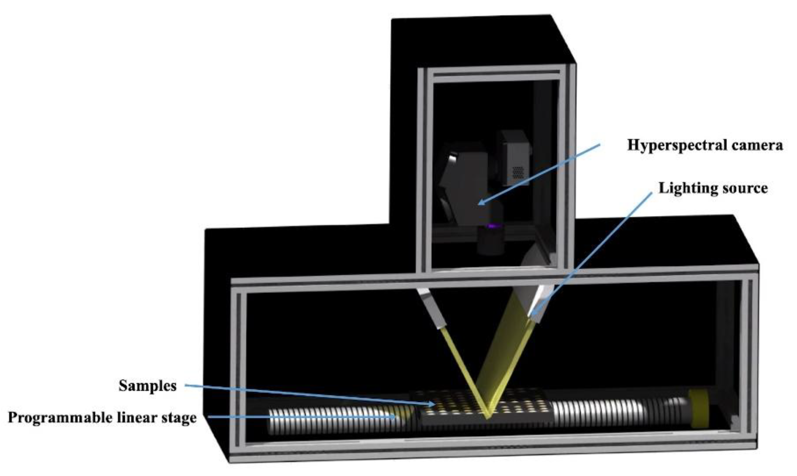
2.2. Hyperspectral Image Acquisition

Hyperspectral images of the rice samples were acquired by using a line-scan (push broom) HSI system as shown in Figure 1. The system consisted of an electron multiplying charge-coupled device camera (EMCCD: Luca R DL-604M, 14-bit, Andor Technology, South Windsor, CT, USA), visible/near-infrared imaging spectrograph (Headwall photonics, Fitchburg, MA, USA), programmable linear stage (translation table) with stepping motor, and light sources. The camera was coupled with a C-mount objective lens (F1.9 35-mm compact lens, Schneider Optics, Hauppauge, NY, USA). The HSI system was constructed to cover visible (VIS) to near-infrared (NIR) wavelengths for reflectance measurements. The lighting sources used were two 150 W halogen lamps with DC power supplies which enabled control of light intensity. Light was transmitted via two optical fibers to the sample surfaces to provide near-uniform illumination. The detailed information of system was described by Kim et al. [28].

Hyperspectral images of rice samples were collected by placing the sample plate onto the programable translation table unit and obtaining spectral/spatial data line-by-line as the translation table moved the sample plate under the instantaneous field of view (IFOV) of the HSI system. The exposure time was set at 16 ms and the samples on the translation table were advanced at 0.3 mm/scan. Thus, to cover the spatial shape of samples (15 cm plate holding 100 samples), a total of 500 steps for advancement of the plate was required. The hyperspectral reflectance images of the rice were stored for further processing and analyses. The white and dark reference images were also acquired after collecting hyperspectral data for individual sample plates. A white reference was obtained using a Spectralon (~99% reflectance), and the dark reference was obtained by capping the objective lens.

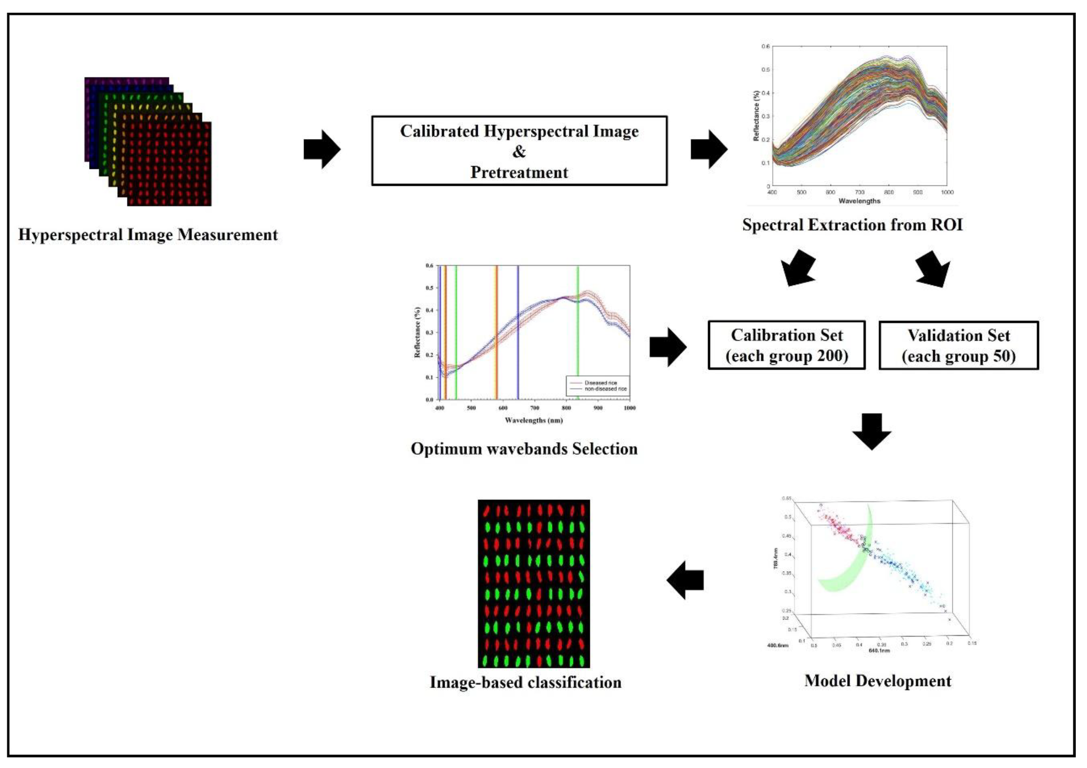
2.3. Data Extraction and Pretreatment of Spectra

In order to extract the actual spectral response of the samples, the influence of both the white and dark current image was removed and thus the calibrated image, I_R, was achieved by the following equation [28].

$$I_R=\frac{I_r-I_d}{I_w-I_d},$$

(1)

where I_r is the sample image, I_d is the dark current image and I_w is the reference image.

The corrected hypercube for each plate (100 samples) was 500 × 502 pixels in the spatial dimension with 128 wavebands spanning 396 to 1004 nm. For the analysis, region of interest (ROI) selection was conducted by a simple thresholding method to remove the background effect of the sample holder so as to visualize only seed pixels. It was not possible to visually select and identify partial ROIs within individual seeds as being a diseased or healthy ROIs, since the number of pixels within the seed area is a small (average of 170 pixels/seed) and the boundary of the diseased region is ambiguous. Therefore, the mean spectrum of each individual seed was calculated to represent the sample. As the next step, an ROI for each seed sample was selected to obtain an averaged spectra for the seed, for further analysis.

In general, spectroscopic data can be affected by baseline shift, light scattering and low signal-to-noise of the system [29]. To mitigate these artifacts, the averaged spectral data of each rice sample was subjected to five different pretreatment methods: standard normal variate (SNV), normalization (mean, maximum and range) and smoothing with three windows sizes. A summary of the equations used in these pretreatment methods is presented in

Table 1. Pretreatment methods and equations.

Normalization	Maximum	$S_{\left(j,k\right)}=\frac{X_{raw\left(j,k\right)}}{X_{max}}$
	Mean	$S_{\left(j,k\right)}=\frac{X_{raw\left(j,k\right)}}{X_{mean}}$
	Range	$S_{\left(j,k\right)}=\frac{X_{\left(j,k\right)}-X_{min}}{X_{max}-X_{min}}$
SNV		$S_{\left(j,k\right)}=\frac{X_{\left(j,k\right)}-A_0}{A_1}$	$A_0$: average value of the sample spectrum $A_1$: standard deviation of the sample-spectrum
Smoothing		$S_{\left(j,k\right)}=\frac{x_{\left(j-1,k\right)}+x_{\left(j,k\right)}+x_{\left(j+1,k\right)}}{3}$

.

2.4. Optimal Feature Selection and Discriminant Analysis

The collected hyperspectral imaging data (hypercube) consists of over 100 contiguous waveband images [11]. In this study, SFS with classifiers was applied to the calibration set to select the optimal wavelengths for building a discriminative model to classify sound and diseased rice seeds. The first step begins with an empty set, and all the variables that have not yet been selected are considered for selection, and their impact on the evaluation score are recorded. At the end of the step, the variables resulting in the best score are included in the set. Then a new step begins, and the remaining variables are considered. This is repeated until a prespecified number of variables has been included [21,22,30]. The optimal wavelengths were selected by performing SFS on the calibration set and repeating until the prespecified number of 10 wavelengths was obtained. An independent validation set was used separately to determine the final generalization performance. The accuracy of the four different classification methods using the SFS selected optimal band pairs was evaluated. The aim of this study was to develop a classification model based on the optimal wavelengths to discriminate sound rice samples from diseased ones. Thus, an SVM-based multivariate classification model and discriminant analysis were considered.

The SVM finds the best hyperplane, known as the decision boundary, in feature dimensional space. The method determines the optimal hyperplane for group separation by the largest margin between groups [26]. In this paper, SVM and SVM with Gaussian radial basis function (RBF) were performed. The SVM finds the linear decision boundary in feature space. To find the non-linear decision boundary in feature space, the SVM with RBF finds the decision boundary in a higher dimensional feature space by using mapping methods. The values of cost function (c) and gamma (γ), which are parameters for building the SVM model, were chosen by a grid search method that scans for optimal parameters for a given model by building a model on all possible parameter combinations.

The LDA usually builds up the model which minimizes the within-group variance while maximizing the between-group variance [24,25,26]. QDA is close to LDA except that a covariance matrix must be estimated for each group. In this case, the decision boundary between groups is non-linear (i.e., quadratic). However, if the training data set does not follow the Gaussian distribution, the LDA and QDA would lead to erroneous results since these methods are based on the concept of Bayes’ theorem [24]. In this investigation, the SVM and discriminant analysis were used for classifying the diseased and sound rice groups. To enhance the generalization and prevent over-fitting, all of the methods were coupled with a 10-fold cross-validation method. All image correction, spectral extraction, preprocessing and modeling were performed using programs developed in MATLAB (MathWorks, Natick, MA, USA). Figure 2 details the procedure used in the data processing.

2.5. Image-Based Classification for Diseased Seed Detection

One of the advantages of hyperspectral imaging is that it provides a visualization map for the samples. With the characteristics of acquiring spatial and spectral information together, the developed classification models (LDA, QDA, SVM, and RBF-SVM) can be applied to hyperspectral images to form classification maps, thereby allowing the rice seeds to be simply classified based on the intensity of the pixels. In this study, the visualization process was performed on the hyperspectral data (background-removed image of rice seeds) by applying the different classification models. The resultant images or visualization maps can then be used to determine the presence of any diseased rice seeds. The diseased rice seeds attained the lower score values, hence, if the same model was applied to the images, the pixel value of diseased samples will be lower than that of the sound samples. Therefore, by thresholding the pixel values, resultant images can be used for discriminating between two groups of samples.

3. Results and Discussion

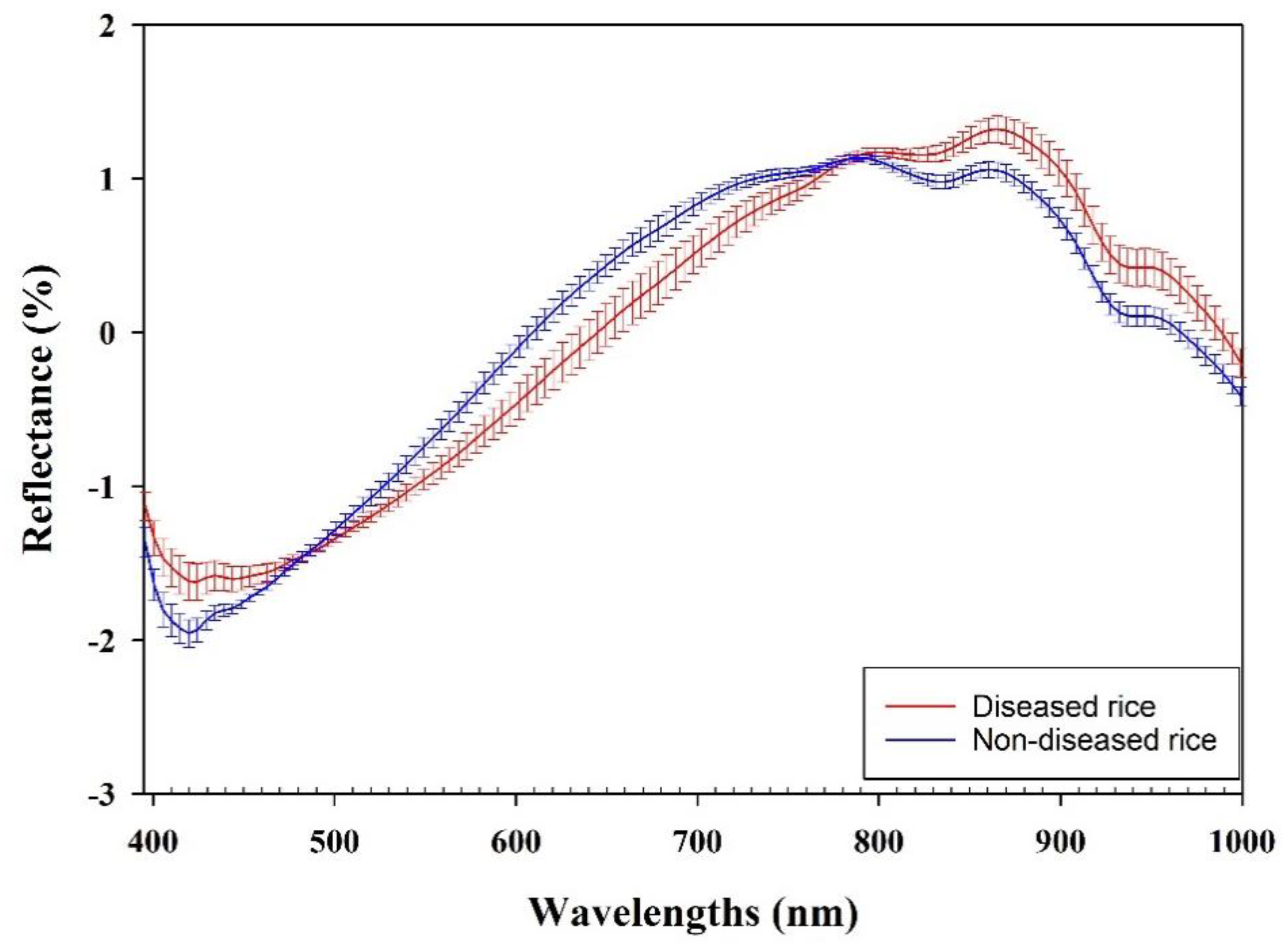
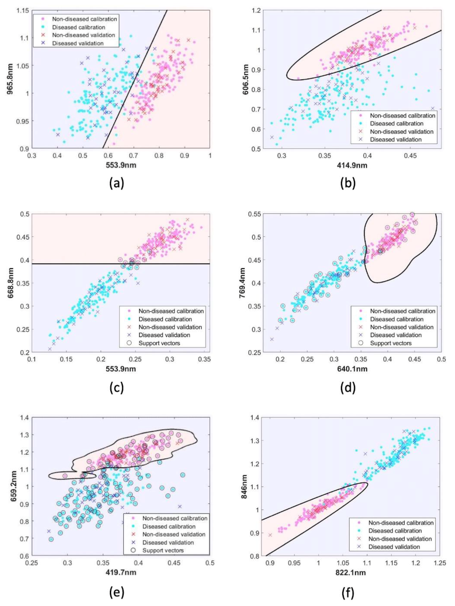
3.1. Spectral Profiles and Selection of Optimal Wavelengths

The average spectra of the sound and diseased rice samples, with SNV pretreatment, are shown in Figure 3. Mean spectra of healthy and diseased seeds in Figure 3 clearly show the spectra are distinguishable, indicating that the mean spectra do not cause error due to non-homogenous spectral grouping as explained by Yousefi et al. (2018) [31]. Distinguished wavelength regions were determined by removing a constant offset term. Aside from the intersections of spectral intensities at around 480 and 760 nm, the sound and diseased rice samples exhibited visually obvious differences throughout entire spectral region under investigation. The obvious differences were generally indicative of the more reddish and less blue color of the diseased rice.

Intensity differences in the region between 800 and 1000 nm were also observed, possibly due to the changes in chemical composition of the seed due to infection [32,33]. In common with the observation of average spectra, one main interval of wavelengths (from 396 to 416 nm) and minor intervals of wavelengths (from 596 to 646 nm) were observed. This result indicates that the violet-blue and orange-red regions are crucial wavelengths to classify the discolored, diseased rice from sound seed using discriminant analysis methods. It should be noted that the SFS selected wavebands match well with the spectral differences between two different groups of seeds as shown in Figure 3. It is interesting to note that despite a significant visual difference in spectral features of sound and diseased seeds in the NIR region (800–1000 nm), the frequency of these being included among the selected wavelengths is relatively lower than those selected in the visible region by SVM. However, SFS analysis with LDA and QDA classifiers along with different preprocessing methods selected the third highest frequency (optimal) wavelengths in the NIR region as shown in

Table 2. Wavelengths of the three most important bands determined by the sequential forward selection (SFS) method following various classifier pretreatments.

Classifier	Pretreatment	1st Band (nm)	2nd Band (nm)	3rd Band (nm)
SVM	Raw	396	554	669
	SNV	458	846	961
	Max normalization	607	621	631
	Mean normalization	396	611	870
	Range normalization	401	640	669
	Smoothing	396	501	664
SVM with RBF	Raw	401	640	769
	SNV	463	468	635
	Max normalization	396	621	674
	Mean normalization	396	401	875
	Range normalization	405	420	659
	Smoothing	401	635	750
LDA	Raw	396	583	741
	SNV	396	453	846
	Max normalization	559	563	865
	Mean normalization	410	765	865
	Range normalization	554	966	985
	Smoothing	396	578	741
QDA	Raw	420	635	640
	SNV	822	846	880
	Max normalization	712	789	899
	Mean normalization	640	918	956
	Range normalization	415	607	827
	Smoothing	420	631	990

. The reason for differently selected wavebands is that discriminant analysis focuses on minimizing variance among group variables (between-scatter matrix) and maximizing class separation (between-scatter matrix). Therefore, NIR regions with relatively small variance were selected by discriminant analysis. The result of the selected optimum wavelengths by each classifier with pretreatments is shown in Table 2. It is a similar result to a previous study regarding fungal infection in rice panicles in that the blue, green and red regions were also used for important feature discrimination of diseased rice [9]. To choose the number of wavelengths, Figure 4 presents the accuracy at each number of features from 1 to 10. As a result, all of the classifiers obtained a high accuracy with >93%. Moreover, all of the classifiers with pretreatments have similar high accuracy when using over two wavelengths. However, for all classification techniques, raw and smoothed data attained slightly higher accuracy than those models developed with other preprocessing methods. It is important to keep the optimal number of variables at a minimum. However, because a lower number of optimal variables can reduce performance accuracy in many cases, each application should carefully consider the tradeoffs. In addition to the accuracy issue, if the system must consider a greater number of wavelengths, it will be more expensive and take a longer time for data processing due to the increased number of device sensors and increased volume of measurement data. As shown in Figure 4, single wavelengths can classify sound and diseased rice samples with high accuracy. However, the use of a single feature can be highly affected by such things as instrumental variables, signal-to-noise ratio and environmental noise. Therefore, in this study, the number of optimal bands considered were two or three wavelengths for further image analysis, as there was no significant difference in classification accuracy when more wavelengths were added.

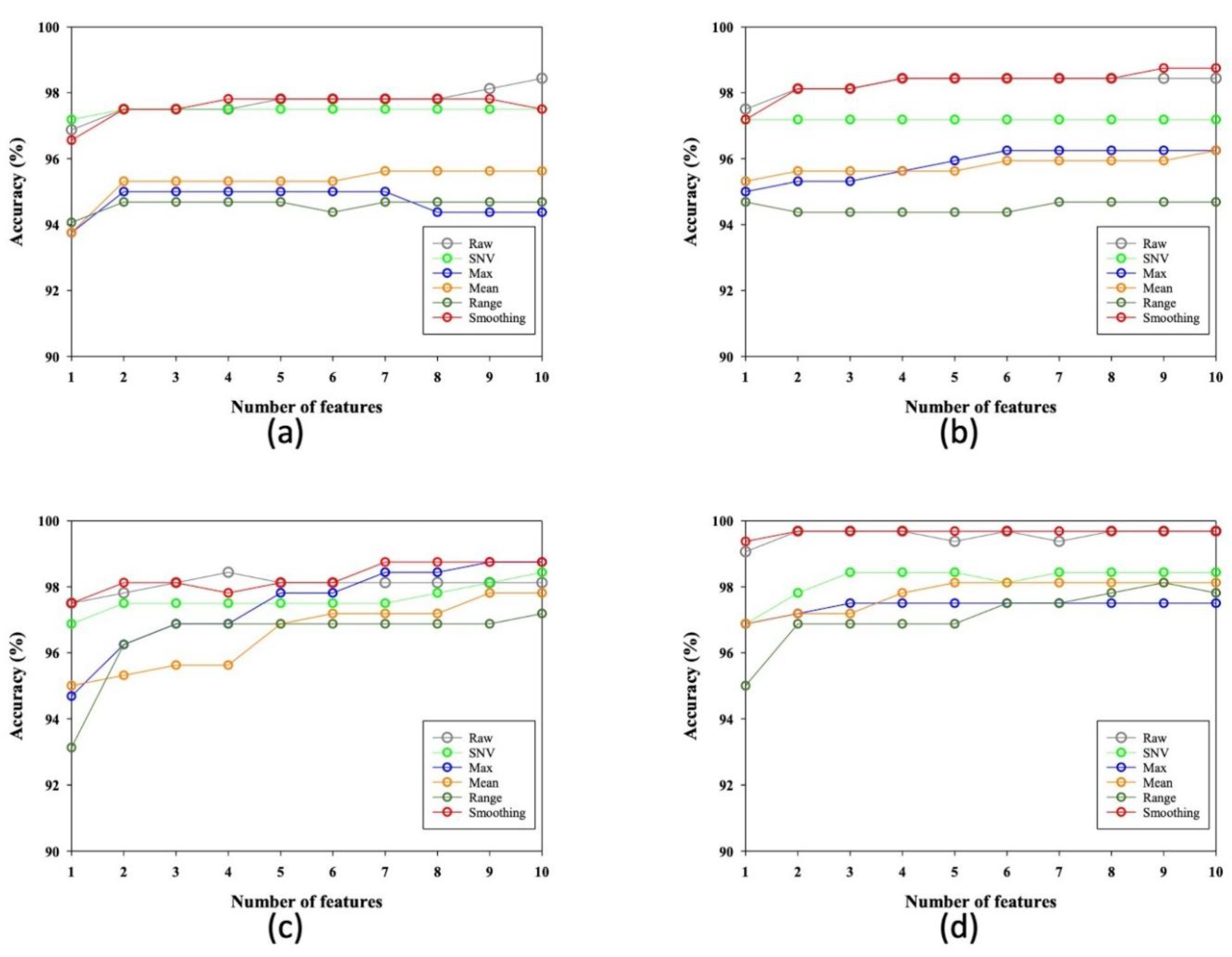
3.2. Classification Models Based on Selected Optimal Wavelengths

Figure 5 shows the visual evaluation of the classification models for overfitting or underfitting, where each decision boundary is shown as a black line between colored regions. A decision boundary with a complex curved shape indicated an overfit model. The decision boundaries of the LDA with range normalization and SVM with raw data models (Figure 5a,c, respectively) are each a simple straight-line and there is as much separation between the two classes as possible. The decision boundaries of QDA with range normalization and RBF SVM with raw data has a curved line. To completely classify the groups, a complicated decision boundary is required which leads to overfitting problems. The decision boundary of QDA and RBF SVM has a simple curve, which means the model is not over-fitted. Thus, most of the validation set samples (identified by ‘x’ markers in Figure 5) belong to the areas that are correctly classified. This result implies that the models are well generalized and will work on an unknown data set. However, in Figure 5f, the distribution of the data is linear indicating the linear decision boundary is a possible classifier for identifying two groups in these two cases. The decision boundary was a relatively more complex curve than a linear decision boundary, even though the validation sets are correctly classified (Figure 5), indicating that it does not guarantee performance using unknown data. The 3D hyperplane decision boundaries for SVM and RBF SVM are shown in Figure 6. The 3D decision boundary for SVM is a flat plane and has a good separation between two groups. However, the 3D decision boundary for RBF SVM consisted of a curved plane even though the distribution of the data is linear. Based on this result, it is not necessary to have a complex shaped model to distinguish between the two groups, and a simple linear or nearly planar decision boundary, as in the case of Figure 5 (when only two features are used), can provide a sufficiently effective and simple model that performs with high accuracy.

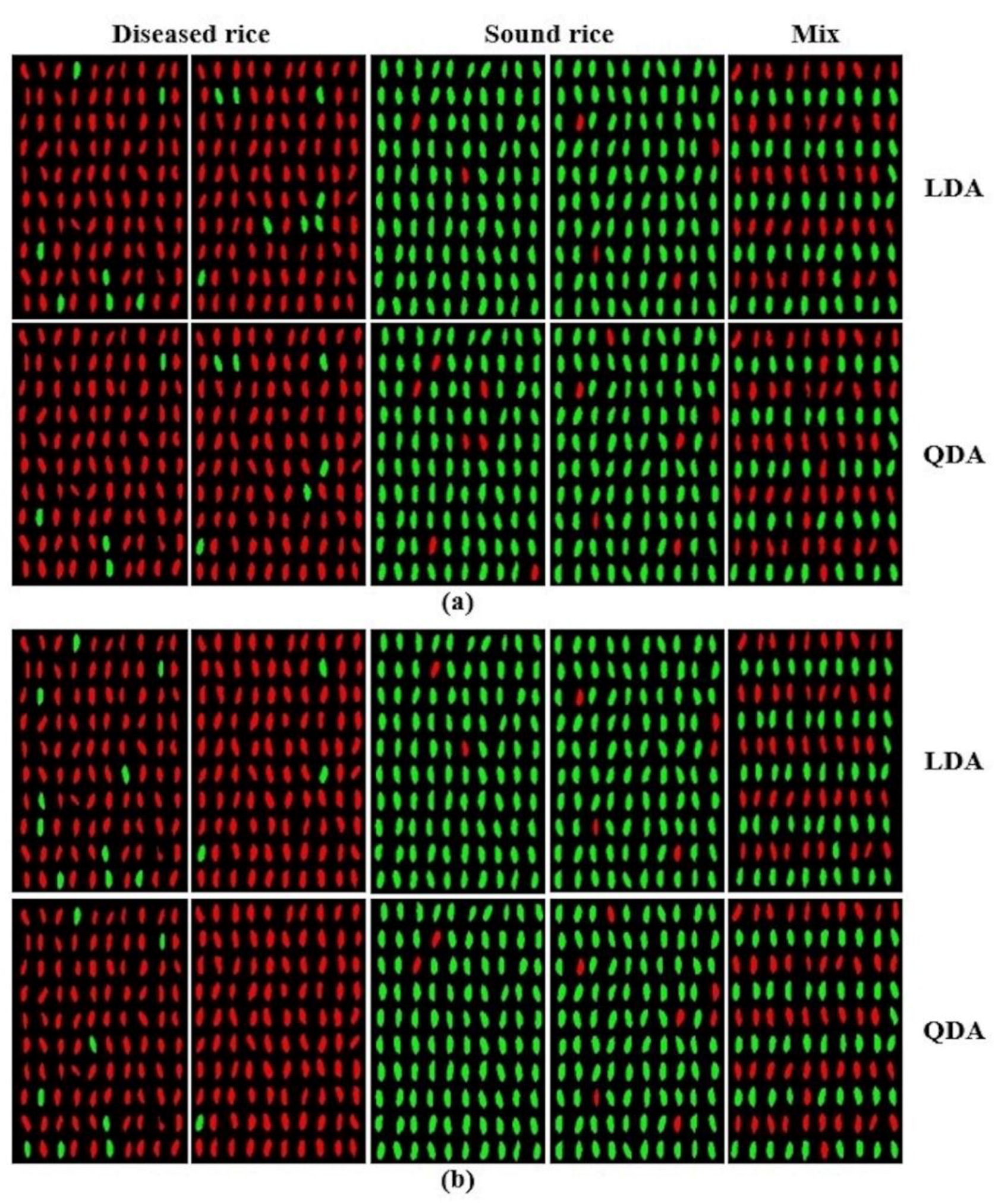
3.3. Image Based Classification

As shown in

Table 3. Calibration and validation results of each classifier with different pretreatment methods using two subset wavelengths for diseased and sound rice seed.

Classifier	Pretreatment	Calibration (%)		Total (%)	Validation (%)		Total (%)
		Diseased	Sound		Diseased	Sound
LDA	RAW	92.5	97	94.8	96	100	98
	SNV	92.5	100	96.3	96	98	97
	Max normalization	94.5	98.5	96.5	98	100	99
	Mean normalization	84.5	100	92.3	96	100	98
	Range normalization	86	99.5	92.8	94	100	97
	Smoothing	92.5	97	94.8	96	100	98
QDA	RAW	95.5	93	94.3	98	92	95
	SNV	92.5	99.5	96	98	100	99
	Max normalization	91	99.5	95.3	94	94	94
	Mean normalization	91	99.5	95.3	94	98	96
	Range normalization	91	99	95	98	100	99
	Smoothing	95	93	94	98	92	95
C-SVM	RAW	96.5	88.5	92.5	98	86	92
	SNV	88.5	99.5	94	94	100	97
	Max normalization	91	99.5	95.3	98	98	98
	Mean normalization	91	99	95	98	100	99
	Range normalization	90	98.5	94.3	94	100	97
	Smoothing	96	89	92.5	98	86	92
SVM with RBF	RAW	96	93.5	95.8	98	92	95
	SNV	89	99.5	94.3	96	100	98
	Max normalization	93.5	96	94.8	98	98	98
	Mean normalization	89.5	100	94.8	96	100	98
	Range normalization	90.5	94.5	92.5	96	92	94
	Smoothing	94.5	93.5	94	98	92	95

and

Table 4. Calibration and validation results of each classifier with different pretreatment methods using three subset wavelengths.

Classifier	Pretreatment	Calibration (%)		Total (%)	Validation (%)		Total (%)
		Diseased	Sound		Diseased	Sound
LDA	RAW	92	95	93.5	96	98	97
	SNV	93	100	96.5	98	98	98
	Max normalization	94	99	96.5	98	98	98
	Mean normalization	88	99.5	93.8	96	100	98
	Range normalization	91.5	99.5	95.5	98	100	99
	Smoothing	93.5	96.5	95	96	100	98
QDA	RAW	95	93.5	94.3	98	94	96
	SNV	94	99.5	96.8	100	98	99
	Max normalization	93	99.5	96.3	98	94	96
	Mean normalization	92.5	98.5	95.5	98	98	98
	Range normalization	93	98.5	95.8	98	98	98
	Smoothing	95.5	95.5	95.5	98	96	97
C-SVM	RAW	96.5	88.5	92.5	98	88	93
	SNV	90.5	99.5	95	94	100	97
	Max normalization	92.5	99	95.8	98	100	99
	Mean normalization	92	98.5	95.3	99.5	100	99.8
	Range normalization	94	98	96	98	98	98
	Smoothing	95.5	87.5	91.5	98	88	93
SVM with RBF	RAW	94	91	92.5	96	90	93
	SNV	95	98.5	96.8	98	98	98
	Max normalization	94	98	96	98	96	97
	Mean normalization	91.5	99	95.3	98	98	98
	Range normalization	93.5	95	94.3	96	98	97
	Smoothing	94	91	92.5	96	90	93

, all four classifiers perform with good accuracy (>92%) for the validation set in all cases. Average classification accuracies of 94% and 96% for the calibration and validation sets, respectively, are achieved when using two wavelengths. When using three wavelengths, the classifiers performed approximately 1% better, with average classification accuracies of 95% and 97% for the calibration and validation sets, respectively. The best performance model was LDA with an accuracy of 96.5% and 99% with max normalization using two wavelengths. The QDA with SNV classifier achieved the best classification accuracies of 96% and 99% for calibration and validation, respectively, when using three wavelengths. The performances of the other classifiers were inferior compared to QDA with SNV but still presented high accuracy for both calibration and validation sets. These models can be used for a practical system.

For using these results on other systems, the LDA and QDA with a smoothing model are suggested since the system chooses optimal wavelengths from diverse regions, not concentrated in one region. Furthermore, previous studies have suggested that using optimal wavelengths for multispectral systems will help retain most of the original information of the samples [15,21,22,34]. However, if a system uses similar wavelength regions, it cannot provide diverse information regarding the target. Hence, by using optimal wavelengths from various regions, it can contain the most possible original information of the target and prevent negative influence resulting from high collinearity. For developing a system for detecting diseased rice, the LDA and QDA with a smoothing model is suggested since wavelengths for LDA and QDA were selected, respectively, in violet, yellow and red regions (396, 578 and 741 nm, respectively) and violet, red, and NIR regions (420, 631 and 990 nm, respectively). This result implies that violet and red regions (yellow, red, orange) have the most significance for identifying diseased rice seed.

In other studies that have used hyperspectral image analysis, colormaps are usually presented with PCA, spectrum angle mapper and normalized cross correlation since they lead to identification of the target [35,36]. Williams et al. (2009) [37] and Juan et al. (2010) [38] depicted maize kernel hardness and sprout damage in Canada western red spring wheat via PCA score. Protein content prediction in single wheat kernels was reported by colormap image with a PLS model [39], and a prediction model based on PLS and genetic algorithm visualized total acid and moisture content in vinegar cultures [40]. These methods are a good way to explain the variance with images in the multivariable data. However, feature extraction methods such as PCA and PLS use full wavelength data, which leads to a longer processing time compared to methods using data consisting of only a few wavelengths. As the purpose of this current study was to minimize the number of spectral bands to increase the detection speed for real-time measurements, it was necessary to select the lowest possible number of spectral variables and to use spectrum data without signal decomposition. Thus, diseased and clean seeds are represented with only two colors in the final detection images that resulted from using either two or three spectral bands.

Pixel values of samples that are less than or equal to the threshold values (0.5) were classified as diseased and they were represented in red in classification images, whereas the green color in the images represents the sound seed samples. The final color-coded images for the calibration and validation sets, based on the LDA and QDA models, are shown in Figure 7. The images clearly show that there were a few kernels in both the diseased and sound rice samples that were misclassified. This could be due to the error in the original subjective sample classification by the experts. Classification of rice seeds by humans takes a longer amount of time, and is a tedious and fatiguing process which is prone to bias and errors. The classification error is an indication that the imaging may be revealing aspects associated with disease that are not apparent to the human eye. The hyperspectral imaging technique can be a potential tool for fast and accurate classification of health/diseased and clean/dirty seeds. The next step of this study is to use a chemical assessment method to verify the results.

4. Conclusions

The present study demonstrated that, with two or three optimized wavelengths, it is possible to develop a highly accurate inspection system for detecting diseased rice grain, in this case likely caused by BPB, using the four discrimination methods. The spectral information from the ROI of the hyperspectral image were acquired and the classification models were developed by using SVM and discriminant analysis. The classification models were based on optimal wavelengths chosen by SFS methods. The combined approaches provided the ability to discriminate between sound and diseased rice seed with accurate results (>91%) for calibration and validation samples. The results suggested that violet and red regions are ideal for development of an objective sorting system that can potentially deal with bulk processing of seeds. Such sorting systems can be used to reduce the use of infected seeds and further mitigate BPB infection during the crop cultivation.

References

1. Mano, H.; Tanaka, F.; Watanabe, A.; Kaga, H.; Okunishi, S.; Morisaki, H. Culturable surface and endophytic bacterial flora of the maturing seeds of rice plants (Oryza sativa) cultivated in a paddy field. Microbes Environ. 2006, 21, 86–100. [Google Scholar] [CrossRef]
2. Kaga, H.; Mano, H.; Tanaka, F.; Watanabe, A.; Kaneko, S.; Morisaki, H. Rice seeds as sources of endophytic bacteria. Microbes Environ. 2009, 24, 154–162. [Google Scholar] [CrossRef] [PubMed]
3. Wamishe, Y.; Kelsey, C.; Belmar, S.; Gebremariam, T.; McCarty, D. Bacterial panicle blight of rice in arkansas about the disease. Agric. Nat. Resour. 2014. Available online: https://www.uaex.edu/publications/pdf/FSA-7580.pdf (accessed on 8 March 2019).
4. Zhou-qi, C.; Bo, Z.; Guan-lin, X.; Bin, L.; Shi-wen, H. Research status and prospect of burkholderia glumae, the pathogen causing bacterial panicle blight. Rice Sci. 2016, 23, 111–118. [Google Scholar] [CrossRef]
5. Mulaw, T.; Wamishe, Y.; Jia, Y. Characterization and in plant detection of bacteria that cause bacterial panicle blight of rice. Am. J. Plant Sci. 2018, 9, 667–684. [Google Scholar] [CrossRef]
6. Ham, J.H.; Melanson, R.A.; Rush, M.C. Burkholderia glumae: Next major pathogen of rice. Mol. Plant Pathol. 2011, 12, 329–339. [Google Scholar] [CrossRef] [PubMed]
7. Mizobuchi, R.; Fukuoka, S.; Tsushima, S.; Yano, M.; Sato, H. QTLs for resistance to major rice diseases exacerbated by global warming: Brown spot, bacterial seedling rot, and bacterial grain rot. Rice 2016, 9, 23. [Google Scholar] [CrossRef]
8. Pinson, S.R.M.; Shahjahan, A.K.M.; Rush, M.C.; Groth, D.E. Bacterial panicle blight resistance QTLs in rice and their association with other disease resistance loci and heading date. Crop Sci. 2010, 50, 1287–1297. [Google Scholar] [CrossRef]
9. Liu, Z.Y.; Wu, H.F.; Huang, J.F. Application of neural networks to discriminate fungal infection levels in rice panicles using hyperspectral reflectance and principal components analysis. Comput. Electron. Agric. 2010, 72, 99–106. [Google Scholar] [CrossRef]
10. Liu, Z.Y.; Huang, J.F.; Tao, R.X. Characterizing and estimating fungal disease severity of rice brown spot with hyperspectral reflectance data. Rice Sci. 2008, 15, 232–242. [Google Scholar] [CrossRef]
11. Qin, J.; Chao, K.; Kim, M.S.; Lu, R.; Burks, T.F. Hyperspectral and multispectral imaging for evaluating food safety and quality. J. Food Eng. 2013, 118, 157–171. [Google Scholar] [CrossRef]
12. Zhang, D.; Zhou, X.; Zhang, J.; Lan, Y.; Xu, C.; Liang, D. Detection of rice sheath blight using an unmanned aerial system with high-resolution color and multispectral imaging. PLoS ONE 2018, 13, e0187470. [Google Scholar] [CrossRef]
13. Van Roy, J.; Keresztes, J.C.; Wouters, N.; De Ketelaere, B.; Saeys, W. Measuring colour of vine tomatoes using hyperspectral imaging. Postharvest Biol. Technol. 2017, 129, 79–89. [Google Scholar] [CrossRef]
14. Yoon, S.C.; Windham, W.R.; Ladely, S.; Heitschmidt, G.W.; Lawrence, K.C.; Park, B.; Narang, N.; Cray, W.C. Differentiation of big-six non-O157 Shiga-toxin producing Escherichia coli (STEC) on spread plates of mixed cultures using hyperspectral imaging. J. Food Meas. Charact. 2013, 7, 47–59. [Google Scholar] [CrossRef]
15. Dai, Q.; Cheng, J.-H.; Sun, D.-W.; Zeng, X.-A. Advances in feature selection methods for hyperspectral image processing in Food industry applications: A review. Crit. Rev. Food Sci. Nutr. 2015, 55, 1368–1382. [Google Scholar] [CrossRef]
16. Cho, B.-K.; Kim, M.S.; Baek, I.-S.; Kim, D.-Y.; Lee, W.-H.; Kim, J.; Bae, H.; Kim, Y.-S. Detection of cuticle defects on cherry tomatoes using hyperspectral fluorescence imagery. Postharvest Biol. Technol. 2013, 76, 40–49. [Google Scholar] [CrossRef]
17. Cho, B.-K.; Chen, Y.-R.; Kim, M.S. Multispectral detection of organic residues on poultry processing plant equipment based on hyperspectral reflectance imaging technique. Comput. Electron. Agric. 2007, 57, 177–189. [Google Scholar] [CrossRef]
18. Qin, J.; Chao, K.; Kim, M.S.; Kang, S.; Cho, B.-K.; Jun, W. Detection of organic residues on poultry processing equipment surfaces by LED-induced fluorescence imaging. Appl. Eng. Agric. 2011, 27, 153–161. [Google Scholar] [CrossRef]
19. Kandpal, L.M.; Lohumi, S.; Kim, M.S.; Kang, J.-S.; Cho, B.-K. Near-infrared hyperspectral imaging system coupled with multivariate methods to predict viability and vigor in muskmelon seeds. Sensors Actuators B Chem. 2016, 229, 534–544. [Google Scholar] [CrossRef]
20. Zhang, W.; Li, X.; Zhao, L. Band priority index: A feature selection framework for hyperspectral imagery. Remote Sens. 2018, 10, 1095. [Google Scholar] [CrossRef]
21. Cen, H.; Lu, R.; Zhu, Q.; Mendoza, F. Nondestructive detection of chilling injury in cucumber fruit using hyperspectral imaging with feature selection and supervised classification. Postharvest Biol. Technol. 2016, 111, 352–361. [Google Scholar] [CrossRef]
22. Vélez Rivera, N.; Gómez-Sanchis, J.; Chanona-Pérez, J.; Carrasco, J.J.; Millán-Giraldo, M.; Lorente, D.; Cubero, S.; Blasco, J. Early detection of mechanical damage in mango using NIR hyperspectral images and machine learning. Biosyst. Eng. 2014, 122, 91–98. [Google Scholar] [CrossRef] [Green Version]
23. Zhang, C.; Guo, C.; Liu, F.; Kong, W.; He, Y.; Lou, B. Hyperspectral imaging analysis for ripeness evaluation of strawberry with support vector machine. J. Food Eng. 2016, 179, 11–18. [Google Scholar] [CrossRef]
24. Wakholi, C.; Kandpal, L.M.; Lee, H.; Bae, H.; Park, E.; Kim, M.S.; Mo, C.; Lee, W.H.; Cho, B.K. Rapid assessment of corn seed viability using short wave infrared line-scan hyperspectral imaging and chemometrics. Sens. Actuators B Chem. 2018, 255, 498–507. [Google Scholar] [CrossRef]
25. Caporaso, N.; Whitworth, M.B.; Grebby, S.; Fisk, I.D. Rapid prediction of single green coffee bean moisture and lipid content by hyperspectral imaging. J. Food Eng. 2018, 227, 18–29. [Google Scholar] [CrossRef]
26. Sanz, J.A.; Fernandes, A.M.; Barrenechea, E.; Silva, S.; Santos, V.; Gonçalves, N.; Paternain, D.; Jurio, A.; Melo-Pinto, P. Lamb muscle discrimination using hyperspectral imaging: Comparison of various machine learning algorithms. J. Food Eng. 2016, 174, 92–100. [Google Scholar] [CrossRef]
27. Teena, M.A.; Manickavasagan, A.; Ravikanth, L.; Jayas, D.S. Near infrared (NIR) hyperspectral imaging to classify fungal infected date fruits. J. Stored Prod. Res. 2014, 59, 306–313. [Google Scholar] [CrossRef]
28. Kim, M.S.; Chen, Y.R.; Mehl, P.M. Hyperspectral reflectance and fluorescence imaging system for food quality and safety. Trans. ASAE 2001, 44, 721–729. [Google Scholar] [CrossRef]
29. Rinnan, A.; van den Berg, F.; Engelsen, S.B. Review of the most common pre-processing techniques for near-infrared spectra. TrAC Trends Anal. Chem. 2009, 28, 1201–1222. [Google Scholar] [CrossRef]
30. Ortaç, G.; Bilgi, A.S.; Taşdemir, K.; Kalkan, H. A hyperspectral imaging based control system for quality assessment of dried figs. Comput. Electron. Agric. 2016, 130, 38–47. [Google Scholar] [CrossRef]
31. Yousefi, B.; Sojasi, S.; Ibarra Castanedo, C.; Maldague, X.P.V.; Beaudoin, G.; Chamberland, M. Continuum removal for ground-based LWIR hyperspectral infrared imagery applying non-negative matrix factorization. Appl. Opt. 2018, 57, 6219. [Google Scholar] [CrossRef]
32. Su, W.H.; He, H.J.; Sun, D.W. Non-destructive and rapid evaluation of staple foods quality by using spectroscopic techniques: A review. Crit. Rev. Food Sci. Nutr. 2017, 57, 1039–1051. [Google Scholar] [CrossRef]
33. Wang, L.; Liu, D.; Pu, H.; Sun, D.-W.; Gao, W.; Xiong, Z. Use of hyperspectral imaging to discriminate the variety and quality of rice. Food Anal. Methods 2015, 8, 515–523. [Google Scholar] [CrossRef]
34. Xiaobo, Z.; Jiewen, Z.; Povey, M.J.W.; Holmes, M.; Hanpin, M. Variables selection methods in near-infrared spectroscopy. Anal. Chim. Acta 2010, 667, 14–32. [Google Scholar] [CrossRef]
35. Yousefi, B.; Sojasi, S.; Castanedo, C.I.; Maldague, X.P.V.; Beaudoin, G.; Chamberland, M. Comparison assessment of low rank sparse-PCA based-clustering/classification for automatic mineral identification in long wave infrared hyperspectral imagery. Infrared Phys. Technol. 2018, 93, 103–111. [Google Scholar] [CrossRef]
36. Singh, C.B.; Jayas, D.S.; Paliwal, J.; White, N.D.G. Detection of insect-damaged wheat kernels using near-infrared hyperspectral imaging. J. Stored Prod. Res. 2009, 45, 151–158. [Google Scholar] [CrossRef]
37. Williams, P.; Geladi, P.; Fox, G.; Manley, M. Maize kernel hardness classification by near infrared (NIR) hyperspectral imaging and multivariate data analysis. Anal. Chim. Acta 2009, 653, 121–130. [Google Scholar] [CrossRef]
38. Xing, J.; Symons, S.; Shahin, M.; Hatcher, D. Detection of sprout damage in Canada Western Red Spring wheat with multiple wavebands using visible/near-infrared hyperspectral imaging. Biosyst. Eng. 2010, 106, 188–194. [Google Scholar] [CrossRef]
39. Caporaso, N.; Whitworth, M.B.; Fisk, I.D. Protein content prediction in single wheat kernels using hyperspectral imaging. Food Chem. 2018, 240, 32–42. [Google Scholar] [CrossRef] [PubMed]
40. Zhao, J.; Shen, T.; Li, G.; Zhu, Y.; Zou, X.; Holmes, M.; Shi, J. Determination of total acid content and moisture content during solid-state fermentation processes using hyperspectral imaging. J. Food Eng. 2015, 174, 75–84. [Google Scholar] [CrossRef]
Figure 1. Schematic of the hyperspectral imaging system.
Applsci 09 01027 g001
Figure 2. Key procedure steps used for the discrimination of diseased rice seed.
Applsci 09 01027 g002
Figure 3. Mean spectra of diseased and sound (non-diseased) rice seeds and standard deviation bars after preprocessing with the standard normal variate (SNV) method.
Applsci 09 01027 g003
Figure 4. Performance comparison of SFS using the classifiers of (a) linear discriminant analysis (LDA); (b) quadratic discriminant analysis (QDA); (c) support vector machine (SVM) and (d) SVM with radial basis function (RBF) kernel, with different data preprocessing methods for two-class classification.
Applsci 09 01027 g004
Figure 5. The decision boundaries are visualized by using two wavelengths. (a,b) show LDA with range normalization and QDA with range normalization. (c,d) show SVM with raw data and RBF SVM with raw data. (e,f) show RBF SVM with range normalization and QDA with SNV.
Applsci 09 01027 g005
Figure 6. The decision boundaries are visualized in raw data for classification between sound and diseased rice samples by using (a) SVM and (b) RBF SVM classification methods with three features.
Applsci 09 01027 g006
Figure 7. Visualization of classification image with smoothing pretreatment by using (a) two and (b) three wavelengths.
Applsci 09 01027 g007