Expanded Douglas–Peucker Polygonal Approximation and Opposite Angle-Based Exact Cell Decomposition for Path Planning with Curvilinear Obstacles


Abstract
1. Introduction
2. Polygonal Approximation Algorithm of Curvilinear Obstacle
2.1. Douglas-Peucker Algorithm
| Algorithm 1. Pseudo Code of the Initial DP. | |
| Input: C ← Set of point lists of the obstacle ε ← Threshold value for maximum dissimilarity tolerance Output: R ← Final result of polygonal approximation of all obstacles represented as a set of point lists | |
| Begin DP Procedure | |
| 1 | for each c in C do |
| 2 | find two points in c, p1 and p2, which have the maximum distance from each other and p1 is in front of p2 |
| 3 | r1 ← recursiveDP(pl[p1 … p2], ε) // pl: point list of a segment of obstacle contour |
| 4 | r2 ← recursiveDP(pl[p2 … starting point of c … p1], ε) |
| 5 | r ← point list[r1[0]… r1[end1 − 1] r2[0]… r2[end2 − 1]] // endi: number of points in ri |
| 6 | insert r to R |
| 7 | end for |
| End DP Procedure | |
| Algorithm 2. Pseudo Code of the Recursive DP. | |
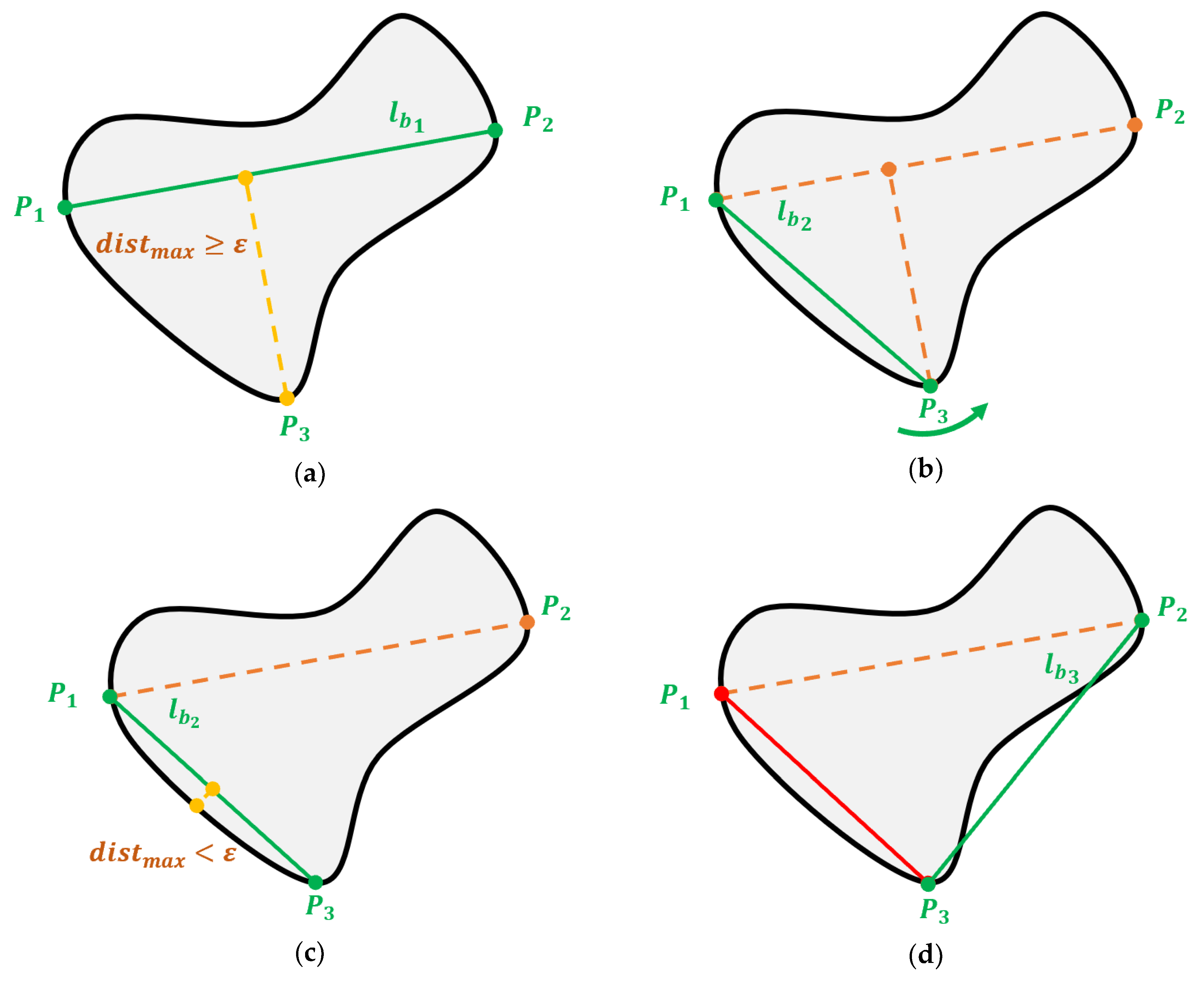
| Input: pl ← Point list of the given curve ε ← Threshold value for maximum dissimilarity tolerance Output: r ← Result of the polygonal approximation of the given curve represented as a point list Initialization: linebase ← line segment connected from pl[0] to pl[end] // end: number of points in pl distmax ← −1 imax ← −1 | |
| Begin recursiveDP Procedure | |
| 1 | for each point p in pl[1…end−1] do |
| 2 | dist ← perpendicular distance between linebase and p |
| 3 | if dist > distmax |
| 4 | distmax ← dist |
| 5 | imax ← index of p |
| 6 | end if |
| 7 | end for |
| 8 | if distmax >= ε then |
| 9 | r1 ← recursiveDP(pl[0…imax], ε) // pl: point list of a segment of the given curve |
| 10 | r2 ← recursiveDP(pl[imax…end], ε) |
| 11 | r ← point list[r1[0]… r1[end1 − 1] r2[0]… r2[end2]] // endi: # of points in ri |
| 12 | else |
| 13 | insert pl[0] to r |
| 14 | insert pl[end] to r |
| 15 | end if |
| End recursiveDP Procedure | |
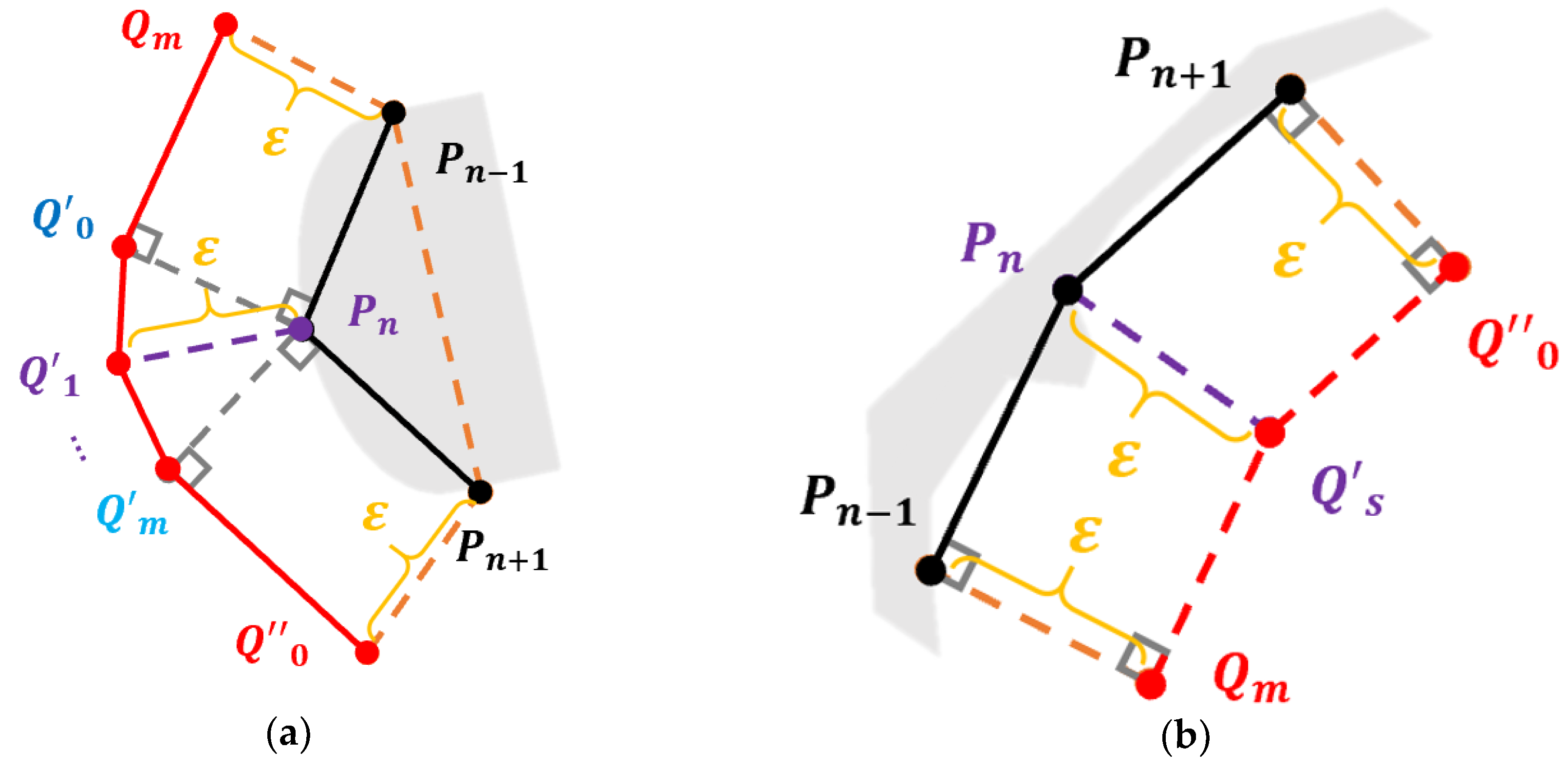
2.2. Proposed Expanded Douglas-Peucker (EDP) Algorithm
| Algorithm 3. Pseudo Code of EDP (Abstract version). | |
| Input: RDP ← Result of DP polygonal approximation of all obstacles represented as a set of point lists ε ← Threshold value for maximum dissimilarity tolerance θrot ← Constant angle for obstacle corner clearance Output: R ← Final result of the EDP polygonal approximation represented as a set of point lists | |
| Begin Expanded-DP Procedure | |
| 1 | for each rDP in RDP do |
| 2 | R ← null |
| 3 | for each point p in rDP do |
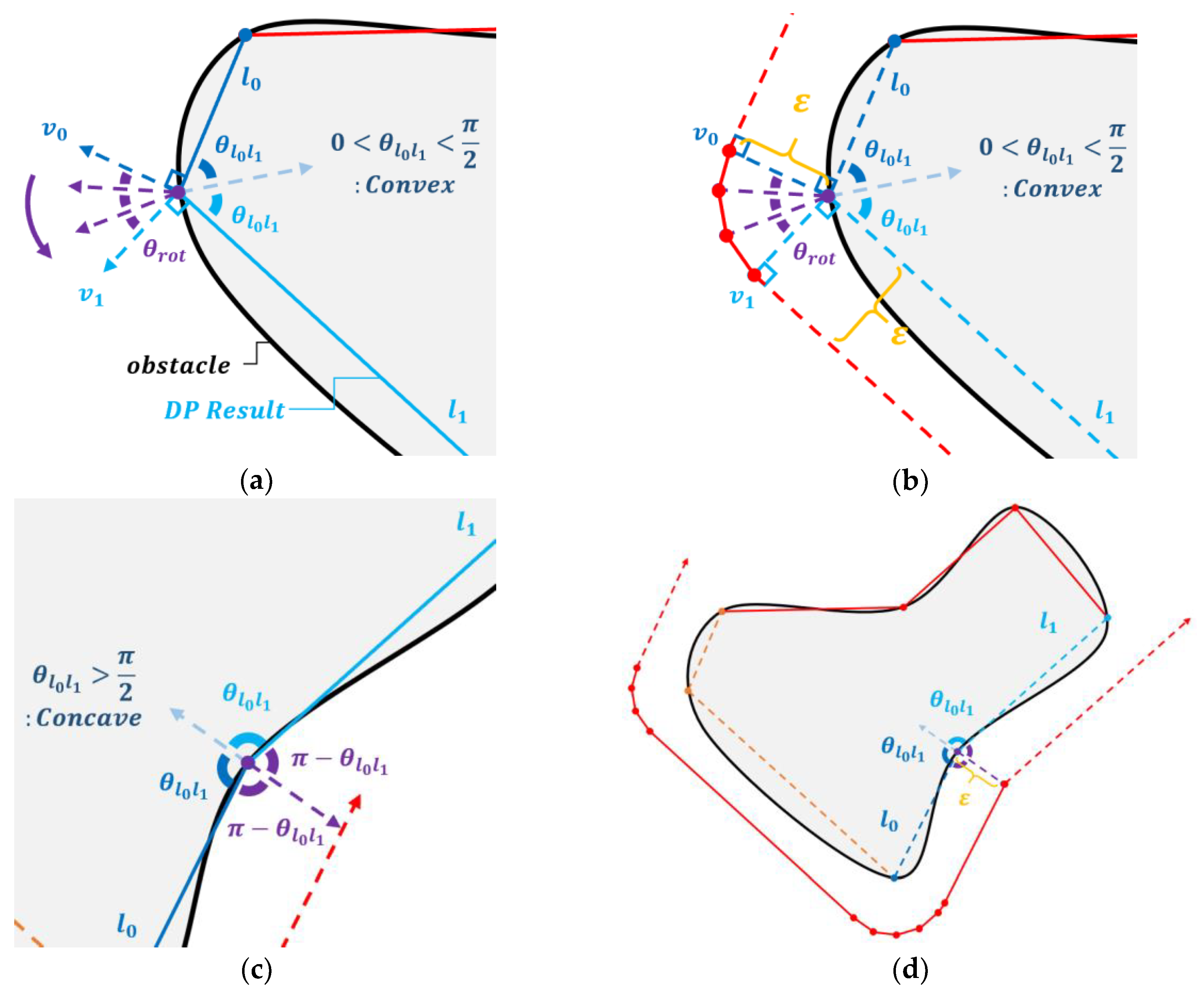
| 4 | if p is convex vertex then |
| 5 | θ ← half inner angle of p |
| 6 | dist ← ε |
| 7 | l0 ← line segment connected from the previous point of p to p |
| 8 | l1 ← line segment connected from p to the next point of p |
| 9 | v0 ← perpendicular half-line to l1 started from p |
| 10 | v1 ← perpendicular half-line to l2 started from p |
| 11 | loop |
| 12 | insert points pcv on the arc with center point p and radius ε, which is consisted of the points according to θrot angle from v0 to v1, to R |
| 13 | end loop |
| 14 | else |
| 15 | θ ← half outer angle of p |
| 16 | dist ← ε/sinθ |
| 17 | insert point pcc far from p with distance dist to the outer direction of the obstacle to R |
| 18 | end if |
| 19 | end for |
| 20 | end for |
| End Expanded-DP Procedure | |
| Algorithm 4. Pseudo Code of EDP (Detailed version). | |
| Input: RDP ← Result of DP polygonal approximation of all obstacles represented as a set of point lists ε ← Threshold value for maximum dissimilarity tolerance θrot ← Constant angle for obstacle corner clearance Output: R ← Final result of the EDP polygonal approximation represented as a set of point lists | |
| Begin Expanded-DP Procedure | |
| 1 | for each rDP in RDP do |
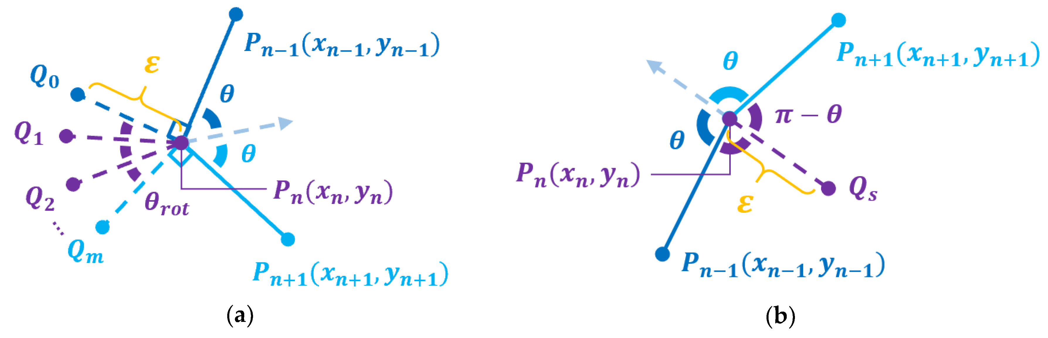
| 2 | for each point Pn(xn, yn) in point list rDP do |
| 3 | if ∠Pn+1PnPn+1 < π then |
| 4 | θ ← ∠Pn+1PnPn+1 |
| 5 | dist ← ε |
| 6 | ← |
| 7 | ← |
| 8 | loop until i |
| 9 | ← |
| 10 | insert to R |
| 11 | i ← i + 1 |
| 12 | end loop |
| 13 | else |
| 14 | θ ← ∠Pn+1PnPn+1 |
| 15 | dist ← ε/sinθ |
| 16 | |
| 18 | insert to R |
| 19 | end if |
| 20 | end for |
| 21 | end for |
| End Expanded-DP Procedure | |
2.3. Mathematical Validation on the Circumscription of the EDP Algorithm
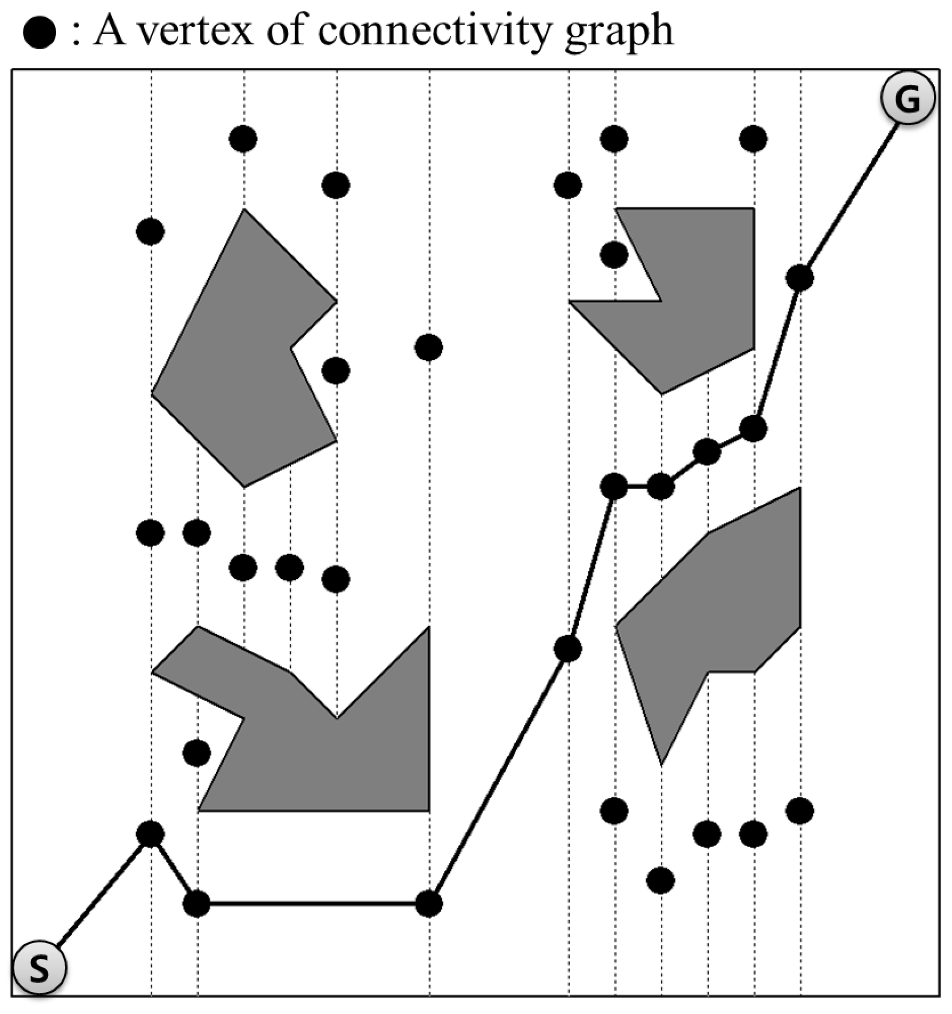
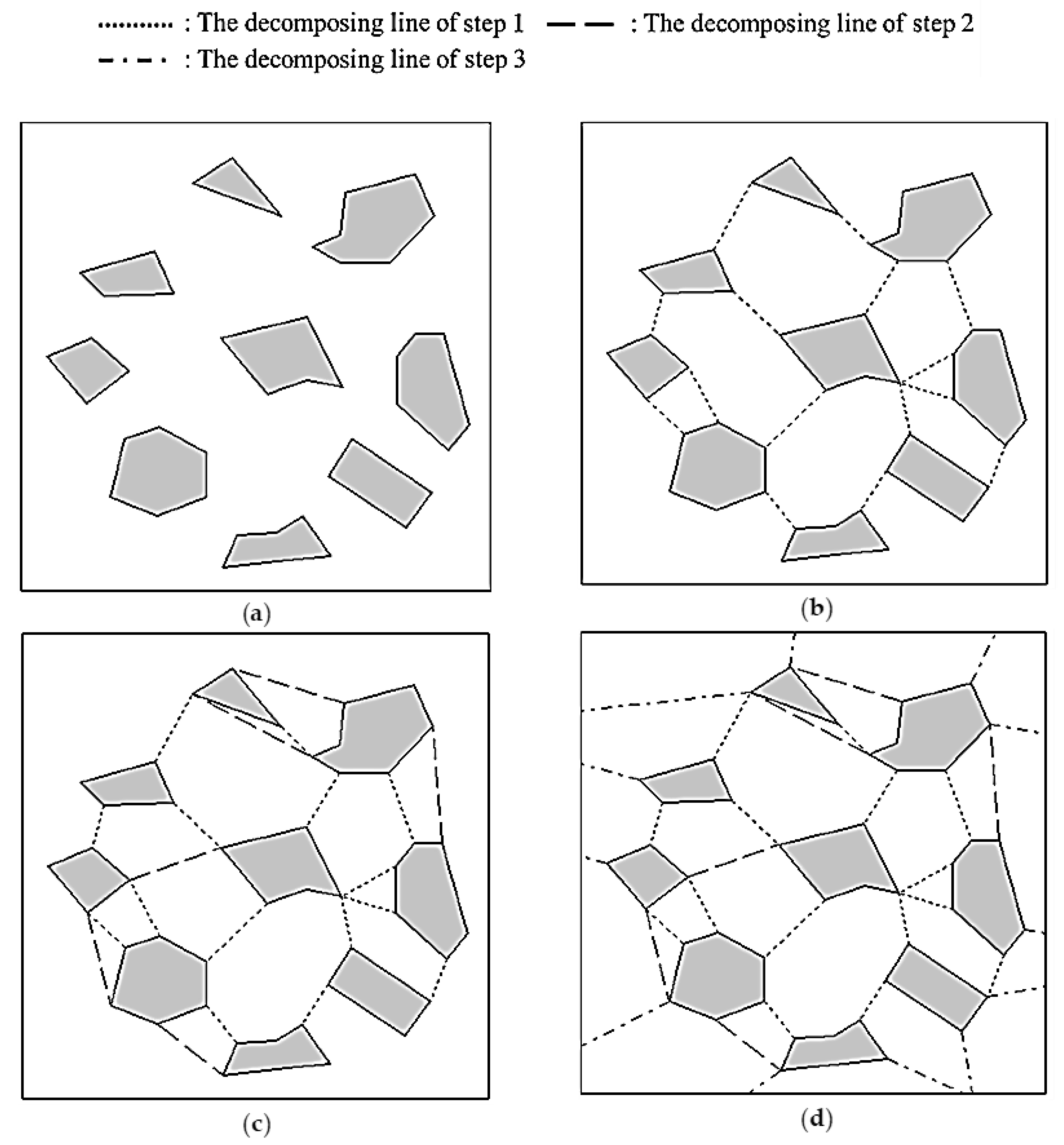
3. Modified Opposite Angle-Based Exact Cell Decomposition (OAECD) Algorithm for Path Planning with Curvilinear Obstacles
| Algorithm 5. Pseudo Code of the modified OAECD (Step 1). | |
| Input: Vc ← R // R: Result of the EDP polygonal approximation of all obstacles represented as a set of point lists M ← Environment map Output: Vchec ← Point set to check for processing M ← Environment map with decomposing lines of step 1 | |
| Begin OAECD-Algorithm Procedure | |
| 1 | for every convex vertex of each obstacle in Vc do |
| 2 | find the closest vertex in the set of all vertices of other obstacles by comparing the distances between the current vertex and other vertices |
| 3 | end for |
| 4 | for each vc1 in Vc do |
| 5 | if there is no decomposing line that is already connected with vc1 then |
| 6 | if va1 is included in the region of the opposite angle of vc1 and line(vc1, va1 in V) is not intersected with other obstacles or other lines then |
| 7 | draw decomposing line from vc1 to va1 and insert vc1 to Vcheck |
| 8 | else if |
| 9 | else if all angles near vc1 are less than or equal to 180° then |
| 10 | insert vc1 to Vcheck |
| 11 | end if |
| 12 | end for |
| End OAECD-Algorithm Procedure | |
| Algorithm 6. Pseudo Code of the modified OAECD (Step 2). | |
| Input: Vc ← R//R: Result of the EDP polygonal approximation of all obstacles represented as a set of point lists M ← Environment map Vcheck ← Point set to check for processing (Result of previous step 1) Output: Vcheck ← Point set to check for processing (Result of this step) M ← Environment map with the decomposing lines of step 1 and 2 | |
| Begin OAECD-Algorithm Procedure | |
| 1 | for each vc2 in Vc - Vcheck do |
| 2 | if there is no decomposing line that is already connected with vc2 then |
| 3 | if va2 has the shortest distance with vc2 compared with those in Vi - {va2} and line(vc2, va2 in Vi) is not intersected with the obstacle and other lines then |
| 4 | draw decomposing line from vc2 to va2 and insert vc2 to Vcheck |
| 5 | end if |
| 6 | else if all angles near vc2 are less than or equal to 180° then |
| 7 | insert vc2 to Vcheck |
| 8 | end if |
| 9 | end for |
| End OAECD-Algorithm Procedure | |
| Algorithm 7. Pseudo Code of the modified OAECD (Step 3). | |
| Input: Vc ← R//R: Result of the EDP polygonal approximation of all obstacles represented as a set of point lists M ← Environment map Vcheck ← Point set to check for processing (Result of previous step 2) Output: M ← The final environment map with decomposing lines of steps 1, 2, and 3 | |
| Begin OAECD-Algorithm Procedure | |
| 1 | for each vc3 in Vc - Vcheck do |
| 2 | if there is no decomposing line that is already connected with vc3 then |
| 3 | draw decomposing line from vc3 in the direction of half angle of the opposite angle of vc3 until it intersects with the boundary of the environment, other obstacles, or other lines and insert vc3 to Vcheck |
| 4 | else if all angles near vc3 are less than or equal to 180° then |
| 5 | insert vc3 to Vcheck |
| 6 | end if |
| 7 | end for |
| End OAECD-Algorithm Procedure | |
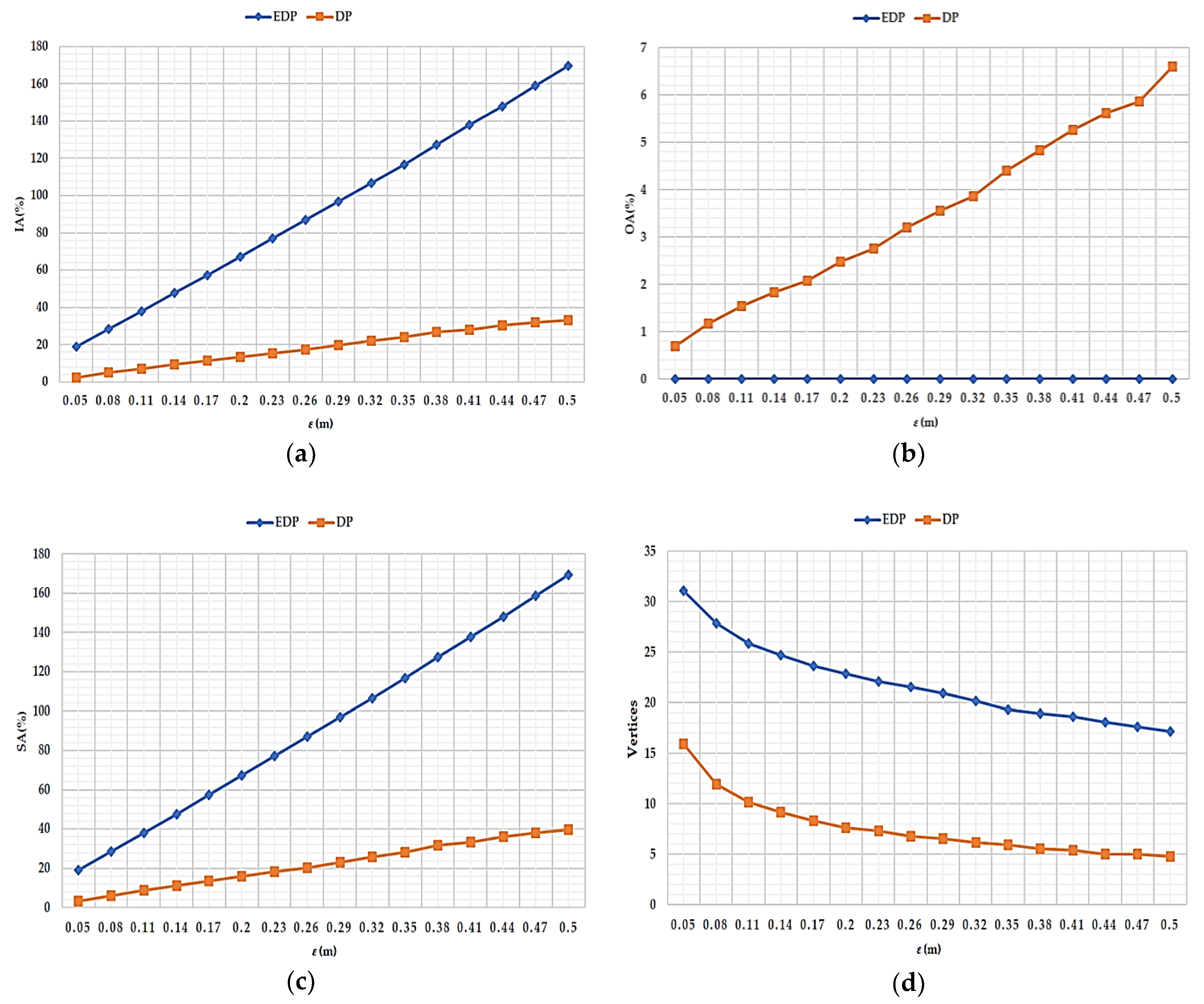
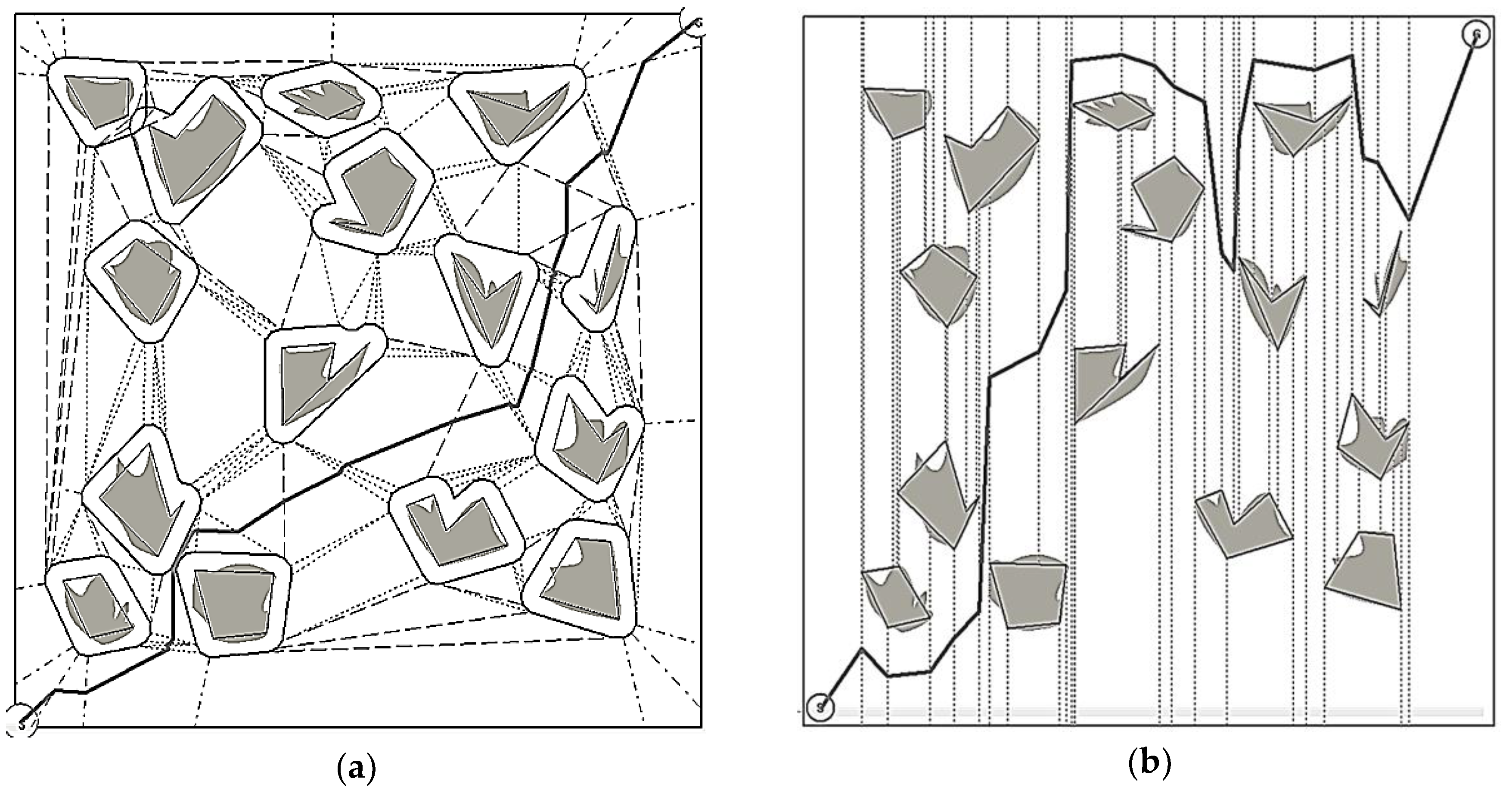
4. Experimental Results
5. Conclusions
Author Contributions
Funding
Conflicts of Interest
References
- Latombe, J.-C. Robot Motion Planning; Kluwer Academic Publishers: Dordrecht, The Netherlands, 1991. [Google Scholar]
- Choset, H.; Lynch, K.M.; Hutchinson, S.; Kantor, G.; Burgard, W.; Kavraki, L.E.; Thrun, S. Principles of Robot Motion: Theory, Algorithms, and Implementations; MIT Press: Boston, MA, USA, 2005. [Google Scholar]
- La Valle, S.M. Planning Algorithms; Cambridge University Press: Cambridge, UK, 2006. [Google Scholar]
- Yang, L.; Qi, J.; Song, D.; Xiao, J.; Han, J.; Xia, Y. Survey of robot 3D path planning algorithms. J. Control Sci. Eng. 2016, 5, 22–44. [Google Scholar] [CrossRef]
- Gonzalez, D.; Perez, J.; Milanes, V.; Nashashibi, F. A Review of Motion Planning Techniques for Automated Vehicles. IEEE Trans. Intell. Transp. Syst. 2016, 17, 1135–1145. [Google Scholar] [CrossRef]
- Yang, H.; Jia, Q.; Zhang, W. An Environmental Potential Field Based RRT Algorithm for UAV Path Planning. In Proceedings of the 2018 37th Chinese Control Conference (CCC), Wuhan, China, 25–27 July 2018; pp. 9922–9927. [Google Scholar]
- Yanyi, Y.; Yingming, Z.; Xingchen, L. An improved artificial potential field algorithm based on nonuniform cell decomposition. In Proceedings of the 2017 6th International Conference on Measurement, Instrumentation and Automation (ICMIA 2017), Zhuhai, China, 29–30 June 2017. [Google Scholar]
- Avnaim, F.; Boissonnat, J.D.; Faverjon, B. A practical exact motion planning algorithm for polygonal objects amidst polygonal obstacles. In Proceedings of the IEEE International Conference on Robotics and Automation, Philadelphia, PA, USA, 24–29 April 1988. [Google Scholar]
- Brooks, R.A.; Lozano-Perez, T. A subdivision algorithm in configuration space for find path with rotation. IEEE Trans. Syst. 1985, 15, 224–233. [Google Scholar]
- Iswanto, I.; Oyas, W.; Imam, C.A. Quadrotor Path Planning Based on Modified Fuzzy Cell Decomposition Algorithm. Telecommun. Comput. Electron. Control 2016, 14, 655–664. [Google Scholar] [CrossRef]
- Nora, S.; Tschichold-Gurmann, N. Exact Cell Decomposition of Arrangements Used for Path Planning in Robotics; Technical Report; ETH Zürich, Department of Computer Science: Zürich, Switzerland, 1999. [Google Scholar]
- Zhang, L.; Kim, Y.J.; Manocha, D. A hybrid approach for complete motion planning. In Proceedings of the International Conference on Intelligent Robots and Systems, San Diego, CA, USA, 29 October–2 November 2007. [Google Scholar]
- Kim, J.-T.; Kim, D.-J. New Path Planning Algorithm based on the Visibility Checking using a Quad-tree on a Quantized Space, and its improvements. J. Inst. Control Robot. Syst. 2010, 16, 48. [Google Scholar] [CrossRef]
- Arney, T. An efficient solution to autonomous path planning by Approximate Cell Decomposition. In Proceedings of the 3rd International Conference on Information and Automation for Sustainability, Melbourne, Australia, 4–6 December 2007. [Google Scholar]
- Rosell, J.; Iniguez, P. Path planning using Harmonic Functions and Probabilistic Cell Decomposition. In Proceedings of the IEEE International Conference on Robotics and Automation, Barcelona, Spain, 18–22 April 2005. [Google Scholar]
- Cowlagi, R.V.; Tsiotras, P. Beyond quadtrees: Cell decompositions for path planning using wavelet transforms. In Proceedings of the 46th IEEE Conference on Decision and Control, New Orleans, LA, USA, 12–14 December 2007. [Google Scholar]
- Ghita, N.; Kloetzer, M. Cell Decomposition-Based Strategy for Planning and Controlling a Car-like Robot. In Proceedings of the 14th International Conference on System Theory and Control, Sinaia, Romania, 17–19 October 2010. [Google Scholar]
- So, B.-C.; Jung, J.-W. Mobile Robot Path Planning with Opposite Angle-Based Exact Cell Decomposition. Adv. Sci. Lett. 2012, 15, 144–148. [Google Scholar] [CrossRef]
- Ramer, U. An iterative procedure for the polygonal approximation of plane curves. Comput. Graph. Image Process. 1972, 1, 244–256. [Google Scholar] [CrossRef]
- Hwang, Y.-S.; Lee, J. Robust 3D map building for a mobile robot moving on the floor. In Proceedings of the 2015 IEEE International Conference on Advanced Intelligent Mechatronics (AIM), Busan, Korea, 7–11 July 2015; pp. 1388–1393. [Google Scholar]
- Gao, H.; Hu, M.; Gao, T. Robust detection of median filtering based on combined features of difference image. Signal Process. Image Commun. 2017, 72, 126–133. [Google Scholar] [CrossRef]
- Douglas, D.; Peucker, T. Algorithms for the reduction of the number of points required to represent a digitized line or its caricature. Can. Cartogr. 1973, 10, 112–122. [Google Scholar] [CrossRef]
- Chazelle, B.; Edelsbrunner, H. An optimal algorithm for intersecting line segments in the plane. In Proceedings of the 29th Annual Symposium on Foundations of Computer Science, White Plains, NY, USA, 24–26 October 1988. [Google Scholar]
- Ravankar, A.; Ravankar, A.; Kobauashi, Y.; Hishino, Y.; Peng, C.-C. Path smoothing techniques in robot navigation: State-of-the-art, current and future challenges. Sensors 2018, 18, 3170. [Google Scholar] [CrossRef] [PubMed]


| ε (m) | EDP (%) | DP (%) | ||||
|---|---|---|---|---|---|---|
| IA | OA | SA | IA | OA | SA | |
| 0.05 | 19.05 | 0.00 | 19.05 | 2.45 | 0.70 | 3.15 |
| 0.08 | 28.46 | 0.00 | 28.46 | 4.89 | 1.17 | 6.06 |
| 0.11 | 37.95 | 0.00 | 37.95 | 7.19 | 1.54 | 8.73 |
| 0.14 | 47.63 | 0.00 | 47.63 | 9.26 | 1.83 | 11.08 |
| 0.17 | 57.34 | 0.00 | 57.34 | 11.50 | 2.08 | 13.58 |
| 0.20 | 67.17 | 0.00 | 67.17 | 13.38 | 2.48 | 15.86 |
| 0.23 | 77.11 | 0.00 | 77.11 | 15.52 | 2.76 | 18.28 |
| 0.26 | 87.01 | 0.00 | 87.01 | 17.23 | 3.20 | 20.43 |
| 0.29 | 96.91 | 0.00 | 96.91 | 19.55 | 3.56 | 23.10 |
| 0.32 | 106.7 | 0.00 | 106.7 | 22.00 | 3.86 | 25.85 |
| 0.35 | 116.7 | 0.00 | 116.7 | 23.90 | 4.40 | 28.30 |
| 0.38 | 127.3 | 0.00 | 127.3 | 26.91 | 4.83 | 31.74 |
| 0.41 | 137.9 | 0.00 | 137.9 | 27.99 | 5.27 | 33.26 |
| 0.44 | 148.0 | 0.00 | 148.0 | 30.57 | 5.62 | 36.19 |
| 0.47 | 158.8 | 0.00 | 158.8 | 32.13 | 5.86 | 37.99 |
| 0.50 | 169.5 | 0.00 | 169.5 | 33.11 | 6.60 | 39.72 |
| AVG | 92.72 | 0.00 | 92.72 | 15.53 | 2.99 | 18.52 |
| ε (m) | Average Number of Vertices | |
|---|---|---|
| EDP | DP | |
| 0.05 | 31.08 | 15.92 |
| 0.08 | 27.87 | 11.92 |
| 0.11 | 25.89 | 10.19 |
| 0.14 | 24.68 | 9.18 |
| 0.17 | 23.67 | 8.33 |
| 0.20 | 22.85 | 7.66 |
| 0.23 | 22.13 | 7.32 |
| 0.26 | 21.55 | 6.83 |
| 0.29 | 20.97 | 6.56 |
| 0.32 | 20.15 | 6.20 |
| 0.35 | 19.32 | 5.91 |
| 0.38 | 18.97 | 5.58 |
| 0.41 | 18.63 | 5.40 |
| 0.44 | 18.06 | 5.06 |
| 0.47 | 17.65 | 5.00 |
| 0.50 | 17.16 | 4.78 |
| AVG | 21.91 | 7.65 |
| (NO, NV) | OAECD | VCD | ||||
|---|---|---|---|---|---|---|
| NV (ea) | VV (ea) | PL (m) | NV (ea) | VV (ea) | PL (m) | |
| (1,10) | 7.60 | 4.30 | 28.43 | 12.00 | 7.00 | 29.27 |
| (3,10) | 19.80 | 6.00 | 29.16 | 36.60 | 16.50 | 33.43 |
| (5,10) | 31.70 | 10.20 | 29.85 | 61.80 | 24.70 | 37.84 |
| (7,10) | 44.10 | 10.60 | 30.37 | 88.20 | 29.90 | 45.89 |
| (9,10) | 56.80 | 11.90 | 29.68 | 111.80 | 34.60 | 47.90 |
| (11,10) | 68.50 | 13.40 | 30.88 | 139.00 | 36.80 | 53.64 |
| (13,10) | 79.20 | 14.90 | 30.62 | 164.70 | 43.80 | 56.38 |
| (15,10) | 92.50 | 17.60 | 30.92 | 192.00 | 45.70 | 48.31 |
| (15,3) | 40.70 | 9.80 | 28.88 | 76.60 | 28.90 | 57.03 |
| (15,5) | 54.90 | 11.10 | 29.72 | 108.00 | 29.80 | 51.94 |
| (15,7) | 69.20 | 13.80 | 29.83 | 141.20 | 37.70 | 59.94 |
| (15,9) | 84.70 | 15.70 | 30.48 | 174.60 | 43.50 | 54.79 |
| (15,11) | 100.60 | 17.60 | 30.82 | 207.80 | 43.00 | 53.86 |
| (15,13) | 116.10 | 21.40 | 31.26 | 249.50 | 46.90 | 58.88 |
| (15,15) | 130.60 | 20.30 | 31.32 | 279.20 | 43.30 | 55.28 |
| AVG | 66.47 | 13.24 | 30.15 | 136.20 | 34.14 | 49.63 |
© 2019 by the authors. Licensee MDPI, Basel, Switzerland. This article is an open access article distributed under the terms and conditions of the Creative Commons Attribution (CC BY) license (http://creativecommons.org/licenses/by/4.0/).
Share and Cite
Jung, J.-W.; So, B.-C.; Kang, J.-G.; Lim, D.-W.; Son, Y. Expanded Douglas–Peucker Polygonal Approximation and Opposite Angle-Based Exact Cell Decomposition for Path Planning with Curvilinear Obstacles. Appl. Sci. 2019, 9, 638. https://doi.org/10.3390/app9040638
Jung J-W, So B-C, Kang J-G, Lim D-W, Son Y. Expanded Douglas–Peucker Polygonal Approximation and Opposite Angle-Based Exact Cell Decomposition for Path Planning with Curvilinear Obstacles. Applied Sciences. 2019; 9(4):638. https://doi.org/10.3390/app9040638
Chicago/Turabian StyleJung, Jin-Woo, Byung-Chul So, Jin-Gu Kang, Dong-Woo Lim, and Yunsik Son. 2019. "Expanded Douglas–Peucker Polygonal Approximation and Opposite Angle-Based Exact Cell Decomposition for Path Planning with Curvilinear Obstacles" Applied Sciences 9, no. 4: 638. https://doi.org/10.3390/app9040638
APA StyleJung, J.-W., So, B.-C., Kang, J.-G., Lim, D.-W., & Son, Y. (2019). Expanded Douglas–Peucker Polygonal Approximation and Opposite Angle-Based Exact Cell Decomposition for Path Planning with Curvilinear Obstacles. Applied Sciences, 9(4), 638. https://doi.org/10.3390/app9040638