Comparative Study of Wind Turbine Placement Methods for Flat Wind Farm Layout Optimization with Irregular Boundary

Featured Application

The comparative results of the effectiveness of different wind turbine placement methods will facilitate the application of a more advantageous method to be used for the wind farm design, and hence improve the cost effectiveness of wind power exploitation.

Abstract

For the exploitation of wind energy, planning/designing a wind farm plays a crucial role in the development of wind farm project, which must be implemented at an early stage, and has a vast influence on the stages of operation and control for wind farm development. As a step of the wind farm planning/designing, optimizing the wind turbine placements is an effective tool in increasing the power production of a wind farm leading to an increased financial return. In this paper, the optimization of an offshore wind farm with an irregular boundary is carried out to investigate the effectiveness of grid and coordinate wind farm design methods. In the study of the grid method, the effect of grid density on the layout optimization results is explored with 20 × 30 and 40 × 60 grid cells, and the means of coping with the irregular wind farm boundary using different wind farm design methods are developed in this paper. The results show that, depending on the number of installed wind turbines, a power output increase from 1% to 1.5% is achieved by increasing the grid density from 20 × 30 to 40 × 60. However, the computational time is more than doubled, rising from 23 h to 47 h with 40 wind turbines being optimized from the coarse grid cells to the densified grid cells. In comparison, the coordinate method is the best option for achieving the largest power increase of 1.5% to 2% (relative to the coarse 20 × 30 grid method), while the least computational time (21 h with 40 wind turbines optimized) is spent.

1. Introduction

Wind energy has attracted extensive attentions for the past few decades as a sustainable energy source. In early days, wind energy was primarily utilized for the household activities, including the grain grinding and water pumping for irrigation [1]. Modern application of utilizing wind resource is mainly for producing electric power [2]. The electric power that is harvested from wind energy is achieved by wind turbines that are placed in cluster to make full use of local wind resources forming a wind farm [3]. However, grouping wind turbines in cluster causes the unavoidable wake interactions, which reduces the total wind farm power output and jeopardizes the wind farm operational performance [4]. Followed by the extraction of kinetic energy from the incoming wind, the wind velocity reduces and it takes tens of kilometers to recover to its original free-stream condition. The air-disturbed area in the flow path is called wake region. When another wind turbine is located inside the wake region of upstream wind turbines, its performance will be greatly affected, which is called the wake effect phenomenon [5]. In order to reduce the wake power losses, wind turbine locations can be optimally chosen based on the contours of the wind farm, the number and size of wind turbines, and the prevailing wind conditions [6].

The study of wind farm layout optimization can be traced back to 1994, when Mosetti et al. [7] studied a 2 km × 2 km square wind farm when considering three types of ideal wind conditions with discrete wind speed/direction. They divided the wind farm with 10 × 10 grid and then used the binary number (0 or 1) to indicate whether the wind turbine exists at a particular grid cell (which is named the grid method). Following this research, Beyer et al. [8] studied the layout optimization of three different types of wind farms using the (x, y) coordinates to represent the wind turbine positions (which is called the coordinate method). Through layout optimization, great improvements in the wind farm power output and economic return have been reported in these two pioneer studies. Over the last decade, a great number of researches on the wind farm optimization have been published. Perez et al. [9] employed the aforementioned coordinate method on an offshore wind farm study while using mathematical programming techniques. Feng and Shen [10] proposed the random search algorithm for the layout optimization of Horns Rev wind farm using the coordinate method. In a paper by Chen et al. [11], a multi-objective genetic algorithm was applied for the optimization studies with two optimization objectives: maximizing the wind farm efficiency and minimizing the cost of energy production. Apart from these studies that apply the coordinate method, others have applied the grid method for the wind farm layout optimization. Zhang et al. [12] proposed the mixed integer programs for optimization using the wind farm grid method and incorporating the complex constraints, including the landowner participation and noise limits. The landowner participation problem is also studied in references [13,14] using the grid method. In addition, Kuo et al. [15] proposed a new mechanistic semi-empirical wake interaction model, while Shakoor et al. [16] proposed a definite point selection technique for wind farm layout optimization studies using the grid method. Due to the representation discrepancy of the wind turbine position for the grid and coordinate methods, their pros and cons are prominent. For the grid method, the available wind turbines locations are fixed with a given grid density, while the number of wind turbines during the optimization running is variable, and hence the optimal wind turbine number can be directly obtained following optimization. The coordinate method fixes the number of wind turbines before conducting optimization, and hence it is more efficient in the optimization under a known wind turbine number.

Though the coordinate method, can theoretically find better results than the grid method with more flexible wind turbine positions, the grid method may narrow the gap of results by increasing the grid density. Given the strong dependence of the results on the optimization formulation, selected algorithm, etc., more in-depth studies are yet to be done by comparing the effectiveness of different wind farm design methods. However, the comparative research of wind farm design methods in literature has been rare. In reference [17], the impact of type of grid cell division on the wind farm optimization results is investigated for the square and circular shape wind farm. Mittal [18] employed a densified grid method (relative to the baseline grid method) for the layout optimization of a square shape wind farm, and an improvement of the optimized wind farm performance is achieved. Wang et al. [19] carried out the comparative study of the grid and the coordinate methods, while the objective wind farm is also an ideal square shape. Above all, previous research on the comparison of different wind farm design methods are all targeting an ideal wind farm with regular boundary shape, based on which the drawn conclusions are probably not eligible for the real wind farm design. Hence, this paper aims to fill the research gap by studying a real two-dimensional wind farm layout optimization with an irregular boundary. In order to investigate the grid method more systematically, two grid densities (coarse 20 × 30 and densified 40 × 60 grid) are studied. When compared to previous research in the literature, the main contributions of this paper are: (1) the comparative study of different wind farm design methods is conducted for a real irregular-boundary wind farm for the first time; and, (2) Means of coping with the boundary constraints using different wind farm design methods are developed, which will shed light on a new perspective for tackling the wind farm optimization with other irregular boundary characteristics.

2. Optimization Models

2.1. Wake Model

For the wind farm optimization, an analytical wake model that quantitatively describes the wake effect should be incorporated into the mathematical formulations. In this paper, the PARK model is applied to quantify the average wind speed in the wake and wake radius behind an upstream wind turbine rotor. Its major characteristic is illustrated in Figure 1 [20].

The original PARK model is proposed by N.O. Jensen et al. [21]. The wake model assumes a linear wind expansion after the wake passes the wind turbine rotor. $r_x$ indicates the wake radius at the axial distance of x, which is given by:

$$r_x=r_0+\alpha x$$

(1)

Based on the theory of momentum conservation, the wind velocity $v_x$ at an axial distance of x downstream of the wind turbine rotor can be calculated by:

$$v_1=v_0\left[1-2a{\left(\frac{r_0}{r_0+\alpha x}\right)}^2\right]$$

(2)

where v₀ is the free stream wind speed and v_x is the wind speed in the wake at the axial distance of x. Notice that the parameter r₀ in the equations is the downstream rotor radius (indicating the radius right behind the wind turbine rotor). According to the actuator disk theory, r₀ is calculated based on the wind turbine rotor radius R as:

$$r_0=R\sqrt{\frac{1-a}{1-2a}}$$

(3)

where a is axial induction factor depicting the induction percent of wind speed reduction. In Equations (1) and (2), α is the entrainment constant that is associated with the surface roughness (z₀) and hub height (h), with the equation of:

$$\alpha =\frac{0.5}{\ln \left(\frac{h}{z_0}\right)}$$

(4)

The velocity deficit (Vel_def) between two wind turbines is calculated by [22]:

$$Vel\_def=2a{\left(\frac{r_0}{r_0+\alpha x}\right)}^2\sqrt{\frac{A_{overlap}}{A_{rotor}}}$$

(5)

where $A_{overlap}$ is the overlapping between the wake and wind turbine rotor. It equals zero without wake interaction and it equals rotor area $A_{rotor}$ with the full wake interaction. For the partial wake interaction, it is calculated according to the relative wind turbine positions [23].

For a wind turbine i that is affected by multiple wakes of up to N wind turbines, the velocity deficit is given by:

$$Vel\_de{f}_i=\sqrt{{\displaystyle \sum _{i=1}^N{\left(\sqrt{\frac{A^i{}_{overlap}}{A^i{}_{rotor}}}2a{\left(\frac{r_0}{r_0+\alpha x_i}\right)}^2\right)}^2}}$$

(6)

The final incoming wind speed of the wake-affected wind turbine is calculated by:

$$v_i=v_0(1-Vel\_de{f}_i)$$

(7)

2.2. Wind Turbine Model and Wind Farm Cost Model

The real wind farm model studied in this paper is an offshore wind farm that is situated in Northern Europe. As reported in reference [24], the Bonus 1 MW wind turbine is installed in the wind farm, and the wind turbine properties are shown in

Table 1. Wind turbine model properties installed in the real offshore wind farm.

Parameters	Values
Rated power	1000 kW
Rotor diameter	54 m
Hub height	60 m
Cut-in wind speed	3 m/s
Rated wind speed	15 m/s
Cut-out wind speed	25 m/s
Turbine power	P = 0.2963U3 kW

(P is the individual wind turbine power output and U is the incoming wind speed magnitude).

There are mainly two types of objective functions for the study of wind farm optimization in the literature, which are the total power output [25,26] and the cost of energy [27,28]. In this paper, Chen’s cost model is introduced for the optimization study and it incorporates a variety of elements that are associated with real wind farm development, such as the market cost, labor cost, etc. [29,30]. The cost model is given by [31]:

$$cost=-0.1539\times P_{\mathrm{r}}-0.001\times N+2\times P_{\mathrm{r}}\times N+0.2504$$

(8)

where the cost unit is in million dollars. P_r is the wind turbine nominal power and N is the wind turbine number. With this model, it can be seen that the wind farm cost is associated with two factors: the wind turbine number and wind turbine rated power. Notice that this cost model is a general expression that describes the real wind farm cost and it is not customized for the current wind farm due to a lack of relevant local-market information. However, since the main focus of this paper is to compare the effectiveness of different wind farm design methods, while the influence of cost model on the comparative study outcomes should be trivial, the utilization of the cost model for the current optimization study should be justified.

2.3. Wind Condition Model

The wind scenario is typically depicted using wind speed and wind direction. In the literature, the simplified wind scenario has been extensively employed for the wind farm layout optimization, which is mainly used for testing the effectiveness of newly proposed methods and techniques, and it mostly incorporates the discrete wind speed/direction description. Realistic description of wind scenario is established on the basis of the measured wind condition data with continuous wind speed/direction variation, and it is commonly accepted that the wind condition variation can be described by the Weibull distribution [32]:

$$f\left(v\right)=\frac{k}{c}{\left(\frac{v}{c}\right)}^{k-1}\exp \left(-{\left(\frac{v}{c}\right)}^k\right)$$

(9)

where f(v) is the probability frequency of wind speed v, c, and k are the scale parameter and shape parameter, respectively. The cumulative Weibull distribution F(v) is given by:

$$F\left(v\right)=1-\exp \left(-{\left(\frac{v}{c}\right)}^k\right)$$

(10)

The wind condition in the real wind farm layout optimization study in this paper is shown in

Table 2. Detail of the Weibull distribution wind condition for the wind farm optimization.

Direction	k	c	ω	Direction	k	c	ω
0°~15°	2	9	0	180°~195°	2	9	0.01
15°~30°	2	9	0.01	195°~210°	2	9	0.01
30°~45°	2	9	0.01	210°~225°	2	9	0.01
45°~60°	2	9	0.01	225°~240°	2	9	0.01
60°~75°	2	9	0.01	240°~255°	2	9	0.01
75°~90°	2	9	0.2	255°~270°	2	9	0.01
90°~105°	2	9	0.6	270°~285°	2	9	0.01
105°~120°	2	9	0.01	285°~300°	2	9	0.01
120°~135°	2	9	0.01	300°~315°	2	9	0.01
135°~150°	2	9	0.01	315°~330°	2	9	0.01
150°~165°	2	9	0.01	330°~345°	2	9	0.01
165°~180°	2	9	0.01	345°~0°	2	9	0.01

. In the current work, 360° wind directions are equally divided into 24 sections with 15° interval. In each of these 24 sections, the wind speed variation is represented by the Weibull distribution, where the probability of occurrence of wind blowing amongst the section is indicated by ω. Obviously, the predominate wind direction is between 75° and 105°. Notice that, although the indicated wind condition is employed for wind farm layout optimization, a finer $3°$ wind direction division (angular resolution) will be applied for power output evaluation analysis due to the reported remark of potentially favorable wind power performance with a resolution coarser than $3°$ in reference [33,34].

3. Methodology

The grid wind farm design method (including two grid densities with 20 × 30 and 40 × 60 grid) and coordinate wind farm design method are applied in this paper for comparative study. In this section, the irregular boundary handling techniques using different design methods, the objective function evaluation method, and the optimization algorithm are introduced.

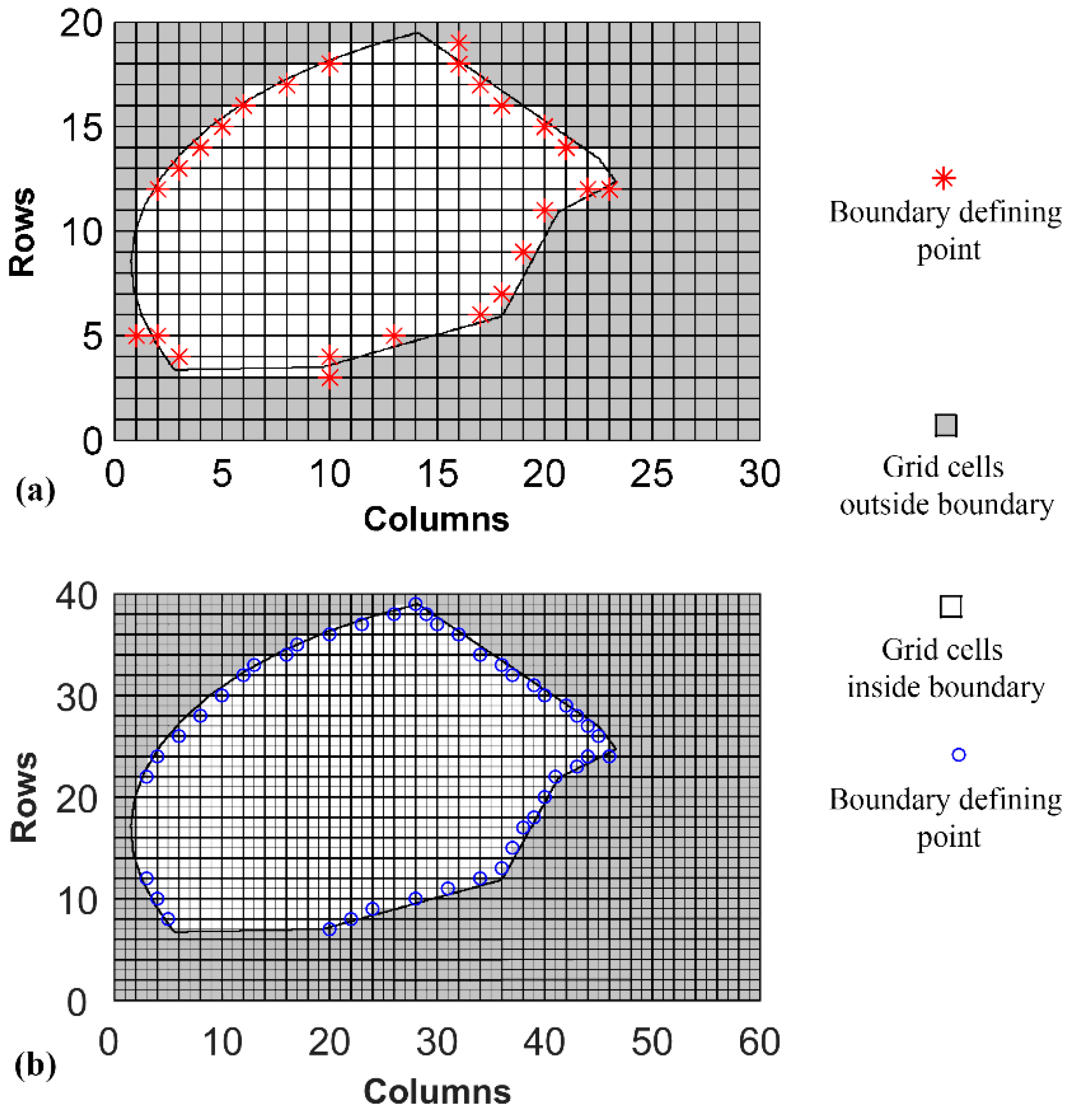
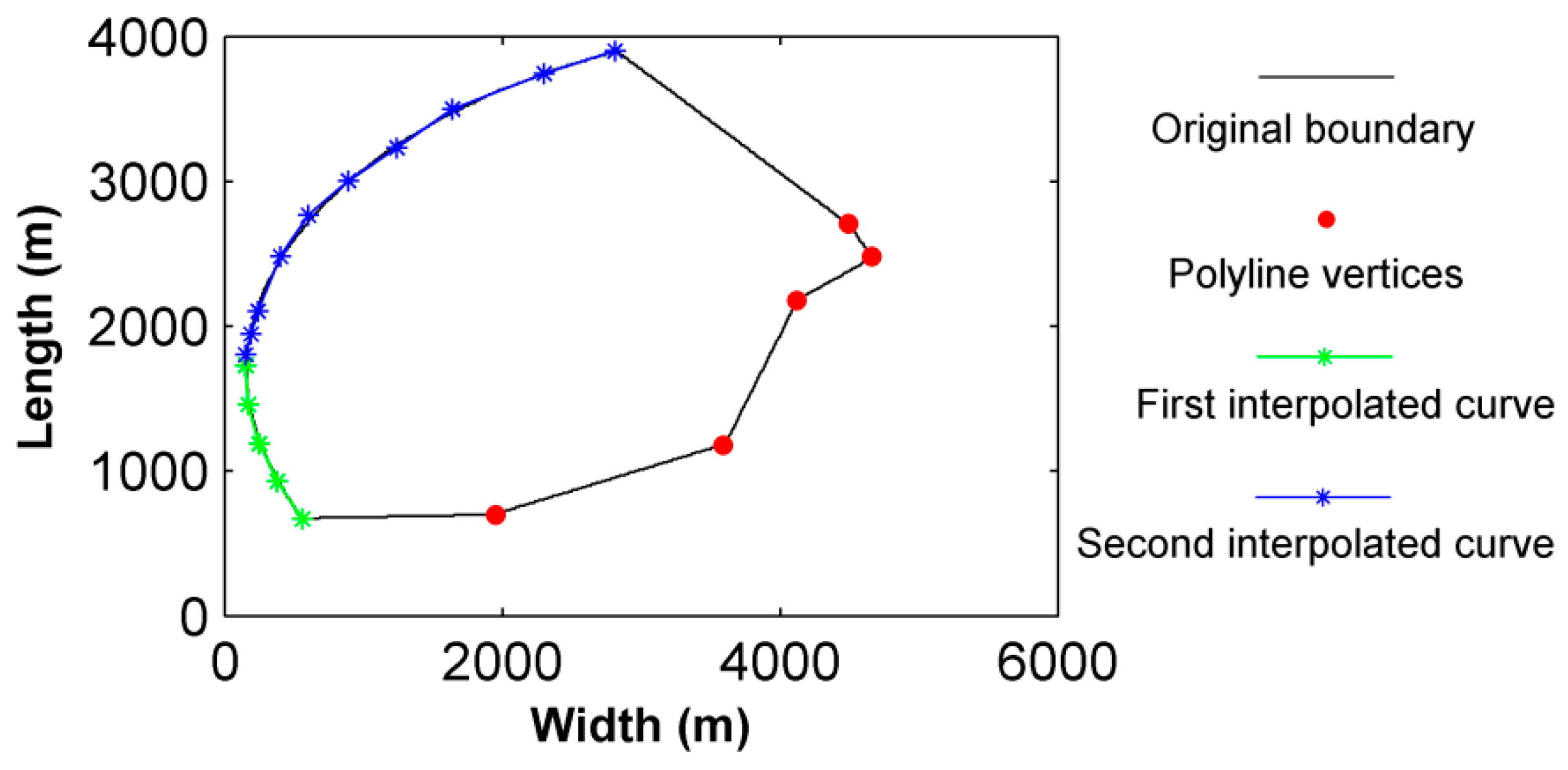
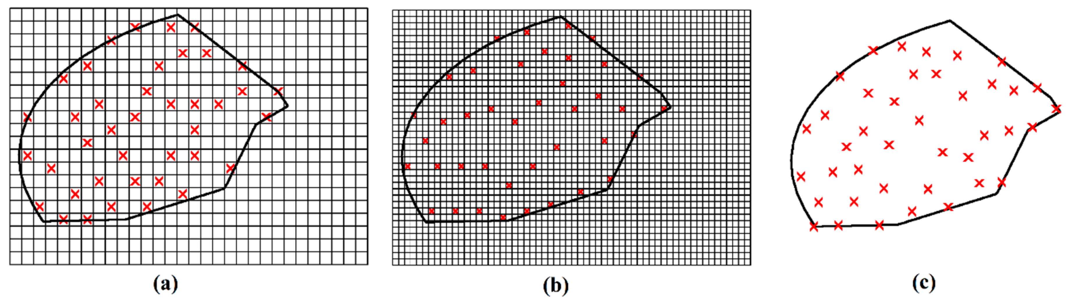
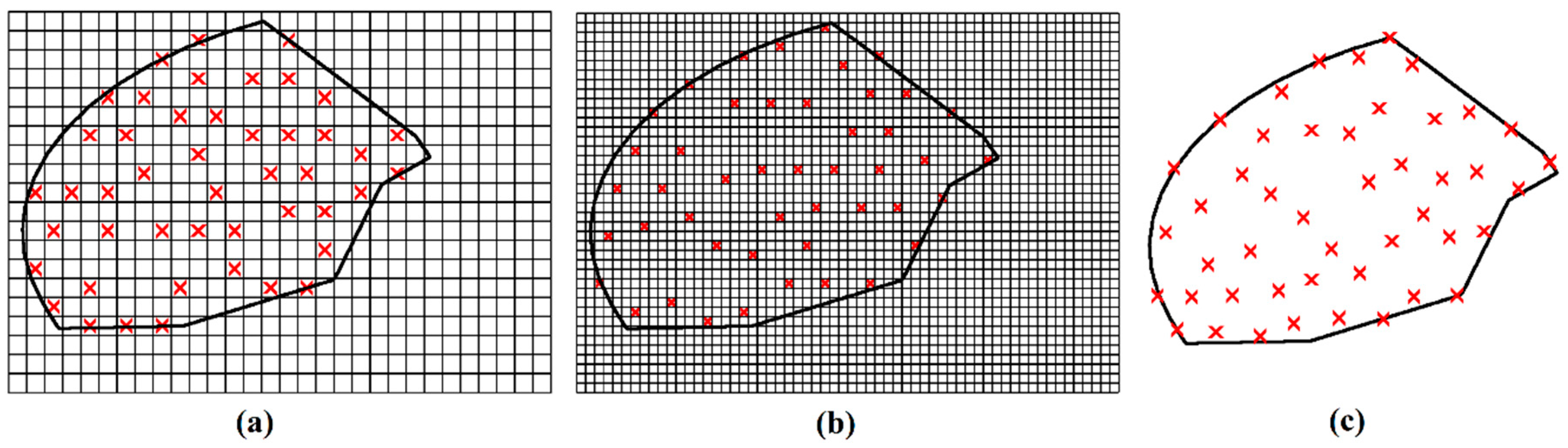
3.1. Boundary Handling Methods

The boundary of studied wind farm is irregular, which is shown in Figure 2, as indicated by the black curved lines. Two different grid densities, i.e., coarse 20 × 30 and refined 40 × 60 grid, are employed, as shown in Figure 2a,b, respectively. The grid cell lengths for the two different divisions are 200 and 100 m, respectively. It is defined that the feasible grid cells are those that are inside the wind farm boundary that can be the potential wind turbine locations, while the infeasible grid cells are those outside the wind farm boundary that cannot be the positions for placing wind turbines. In order to guarantee that the wind turbines are placed within the wind farm boundary for final solutions, the infeasible grid cells are combined into a number of larger rectangles with different sizes. These artificially selected rectangles are made to facilitate the optimization coding, and they are determined by the boundary defining point P_i (red color asterisk points in Figure 2) and one of the four vertices of the whole wind farm boundary as the rectangle diagonal. In this manner, the infeasible grid regions can be determined by the range of row and column indices of these rectangles. Reflected by the number of boundary defining points for the two different grid densities, there are 25 rectangles in total for the 20 × 30 grid, while there are 43 rectangles for the 40 × 60 grid. As can be anticipated, the number of infeasible rectangles increases with more a densified grid. More infeasible rectangles that are inappropriate for locating wind turbines will enable the optimization to be subject to a more complex boundary constraint, which leads to an increasingly high computational burden. Given the significant increase in computational cost, grid cells that are denser than 40 × 60 are not included in the comparative study of this paper.

Unlike the boundary representation using the grid method, Figure 3 shows an alternative way to represent the irregular boundary while using the coordinate method. To facilitate the mathematical coding of the wind farm boundary representation, the left portion of the boundary curve is approximated by interpolated polylines. In order to increase the accuracy of the interpolation polylines, the left portion boundary is divided into two interpolated curves by polynomial approximation: y₁(x) (blue color in Figure 3) and y₂(x) (green color in Figure 3). These two interpolation polylines are connected with the interpolation points (shown as the asterisk points in the figure). As can be seen, the difference between the original boundary and the interpolated polylines is small, which justifies the accuracy of this approximation process. In comparison, the right portion of the boundary is directly the polyline p {(X1, Y1), (X2, Y2), …, (X7, Y7)}, which can be determined by connecting these vertex points (shown as the dot points in Figure 3). For i-th wind turbine with the x coordinate x_i, define a feasible interval of y values that is located inside the wind farm boundary as:

$${\mathcal{C}}_{}\left(x_i\right)=\left\{z|y_{\ell }\left(x_i\right)\le z\le y_u\left(x_i\right)\right\}$$

(11)

where $y_{\ell }\left(x_i\right)$ is the lower bound and $y_u\left(x_i\right)$ is the upper bound at the coordinate $x_i$, and $X=x_1{y}_1{x}_2{y}_2\dots x_N{y}_N$ is comprised of the coordinates of wind turbines (with 2N variables in total). The feasible wind farm layout ensures that all the wind turbine positions are among the feasible intervals. Hence, it satisfies:

$$\sum _{i=0}^N\varphi \left(X,i\right)=0$$

(12)

in which, the further definition is made as:

$$\varphi \left(X,i\right)=\{\begin{array}{cc}1& y\notin {\mathcal{C}}_{}\left(x_i\right)\\ 0& y\in {\mathcal{C}}_{}\left(x_i\right)\end{array}$$

(13)

In comparison to the constraint handling method for the grid method, the formulations of constraint handling for coordinate method are much more straightforward and are hence less computationally intensive. The lower and upper bounds of the y coordinates restrict the wind turbine locations inside the wind farm boundary.

3.2. Comparison of Grid and Coordinate Methods

The selection of wind farm design methods (including selection of grid densities) only affects the means of representation of wind turbine positions. For instance, the wind turbine positions are continuously depicted by Cartesian coordinates in the coordinate method. For the i-th wind turbine in the wind farm, its position is represented by $\left(x_i,y_i\right)$. In comparison, the representation of the wind turbine positions is discrete and determined by the grid divisions/densities for the grid method. For the i-th wind turbine in the wind farm, its row and column indices are $m_i$ and $n_i$, respectively. When choosing the 20 × 30 grid, the row index value is between 1 and 20, while the column index value is between 1 and 30. There are 600 available places for locating wind turbines and the minimal interval of available wind turbine positions is 200 m in both the X and Y directions. When choosing the 40 × 60 grid, the row index value is between 1 and 40, while the column index value is between 1 and 60. In total, there are 2400 available places for locating wind turbines and the minimal interval is 100 m. When the grid cells are further refined, there will be more available places and the less minimal interval. Based on the row and column indices for the grid method, the x and y coordinates of wind turbines are calculated as the product of the indices and the interval.

Though the coordinate method has the prominent advantage in the representation of wind turbine positions from concept, the wind turbine number is fixed in one optimization running, and hence it requires repetitive running to obtain the optimal number of wind turbines. Instead, the grid method can simultaneously optimize the wind turbine positions and the number of wind turbines in one optimization running, and hence it is more advantageous in this regard. Note that, except for the difference of representation of wind turbine positions, the subsequent steps of evaluating the wind farm power output (or objective function) in Section 3.3 are the same for the different wind farm design methods.

3.3. Objective Function Evaluation Method

According to the wind turbine positions (as represented in the form of Cartesian coordinates), the velocity deficits of all wind turbines for different incoming wind directions are calculated based on the introduced analytical wake model.

For the Weibull distribution wind condition, it has been confirmed that only the scaling parameter c is modified by the wake effect, which is given by [32]:

$$c_i\left(\theta \right)=c\left(\theta \right)\times \left(1-Vel\_de{f}_i\right),i=1,2\dots ,N$$

(14)

where c($\theta$) is the scale parameter on the wind direction $\theta$ and Vel_def_i is the velocity deficit on i-th wind direction. The expected individual wind turbine power output P_i under the Weibull distribution wind condition can be represented by:

$$P_i={\displaystyle \underset{0}{\overset{360}{\int }}{{\displaystyle p}}_{\theta }}(\theta ){\displaystyle \underset{0}{\overset{\infty }{\int }}P(v)}\frac{k(\theta )}{c_i(\theta )}{\left(\frac{v}{c_i(\theta )}\right)}^{k(\theta )-1}\exp \left(-{\left(\frac{v}{c_i(\theta )}\right)}^{k(\theta )}\right)\mathrm{d}\theta \mathrm{d}v$$

(15)

where $p_{\theta }\left(\theta \right)$ is the probability of wind blowing on the wind direction $\theta$, $k\left(\theta \right)$ is the shape parameter on the wind direction $\theta$, and $P\left(v\right)$ is the wind turbine power output on wind speed $v$. By the discretization of both wind speeds and wind directions, the individual wind turbine power can be mathematically formulated, which consists of two parts. When the wind speed is beyond the rated speed, the expected power P₁ is given by:

$$P_1=P_{rated}{\displaystyle \sum }_{l=1}^{N_{\theta }}\left\{{\omega }_{l-1}\left(\exp \left(-{\left(\frac{2v_{rated}}{c_i\left(l-1\right)+c_i\left(l\right)}\right)}^k\right)-\exp \left(-{\left(\frac{2v_{cut-out}}{c_i\left(l-1\right)+c_i\left(l\right)}\right)}^k\right)\right)\right\}$$

(16)

where $N_{\theta }$ is the total number of divided wind direction sectors and ${\omega }_{l-1}$ is the probability of a specific wind direction interval of (θ_l−1, θ_l). $c_i\left(l-1\right)$ and $c_i\left(l\right)$ are the wake-affected scale parameter of the corresponding wind directions, respectively. Between the cut-in and the rated wind speeds, the expected power output P₂ is given by:

$$\begin{gathered} P_2={\displaystyle \sum }_{j=1}^{N_v+1}0.2963{\left(\frac{v_{j-1}+v_j}{2}\right)}^3{\displaystyle \sum }_{l=1}^{N_{\theta }}\left\{{\omega }_{l-1}\right(\exp (-{\left(\frac{2v_{j-1}}{c_i\left(l-1\right)+c_i\left(l\right)}\right)}^k) \\ -\exp (-{\left(\frac{2v_j}{c_i\left(l-1\right)+c_i\left(l\right)}\right)}^k)\left)\right\} \end{gathered}$$

(17)

where N_v is the total number of wind speed discretization bins and ω_l−1 is the probability of the wind direction amongst the interval of (θ_l−1, θ_l). The individual wind turbine power is calculated by the aggregation of the two separate power parts by [35]:

$$P_i=P_1+P_2$$

(18)

By substituting the wind farm cost (cost) and the total expected power output (P_tot) into the CoE equation, the substituted CoE function is given by:

$$\mathrm{CoE}=(-0.1539\times P_{\mathrm{r}}-0.001\times N+2\times P_{\mathrm{r}}\times N+0.2504)/{\displaystyle \sum _{i=1}^N{P}_i}$$

(19)

where P_r is the wind turbine nominal power and N is wind turbines number. The optimization function can be mathematically represented as follows and the minimum distance between wind turbines, $d_{min}$, is set to be 7D (D is wind turbine diameter) in this paper.

$$\begin{array}{ll}\mathrm{Minimize}:& \mathrm{CoE}=cost/P_{\mathrm{tot}}\\ \mathrm{Subject}\mathrm{to}:& \begin{array}{}\\ {\displaystyle \sum _{i=0}^N}\varphi \left(X,i\right)=0& (\mathrm{boundary}\mathrm{constraint})\\ \sqrt{{\left(x_j-x_i\right)}^2+{\left(y_j-y_i\right)}^2}\ge d_{\min }(\mathrm{for}\forall i\mathrm{and}j,i\ne j)& (\mathrm{proximity}\mathrm{constraint})\end{array}\end{array}$$

(20)

Besides the objective function (CoE) that is optimized in the paper, it should also be mentioned that the wind farm design methods tested could be incorporated into any objectives of the wind farm layout optimization problem so long as the objective function is mathematically formulated. For instance, the wind farm fatigue load is estimated with a stochastic model in reference [36]. By applying the proposed wind farm design methods (grid or coordinate method) with a different optimization objective, such as the wind farm fatigue load hypothetically, the optimal wind farm layouts can be achieved in the same manner.

In this paper, single objective genetic algorithm (SOGA) is employed as the optimization algorithm for different wind farm design methods studied. SOGA is a metaheuristic algorithm and it is performed while mimicking the natural selection process. It searches problems by relying on bio-inspired operators, including mutation, crossover, and selection [37]. The setting of genetic algorithm (GA) parameters that are used for the optimization using different wind farm design methods in this paper are summarized in

Table 3. Setting of genetic algorithm (GA) parameters of the wind farm layout optimization using different design methods.

	Design Methods	Grid Method (20 × 30 grid)	Grid Method (40 × 60 grid)	Coordinate Method
Parameters
Population type		Binary	Binary	Real
Number of variables		600	2400	2 N
Population size		600	600	600
Generations		1 million	0.5 million	0.5 million

N is number of wind turbines.

. Regardless of the wind farm design methods, the same scattered crossover operator with a rate of 0.8 and the same bit-flip mutation operator with a rate of 0.1 are employed for GA optimization. Attributed to the utilization of C++ compiler platform for the program coding, more GA optimization generations are possible to facilitate the search for the global optimization of wind turbine positions. In this paper, at least half a million generations (for densified grid method) are run for the optimization study and the GA optimization will be terminated once it reaches the predefined maximum generation number.

4. Results and Discussion

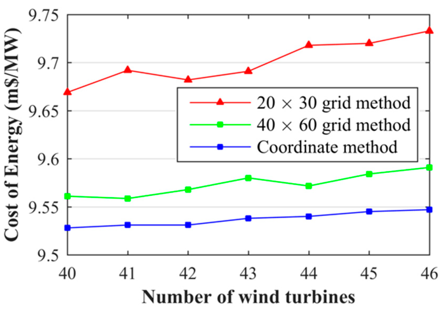
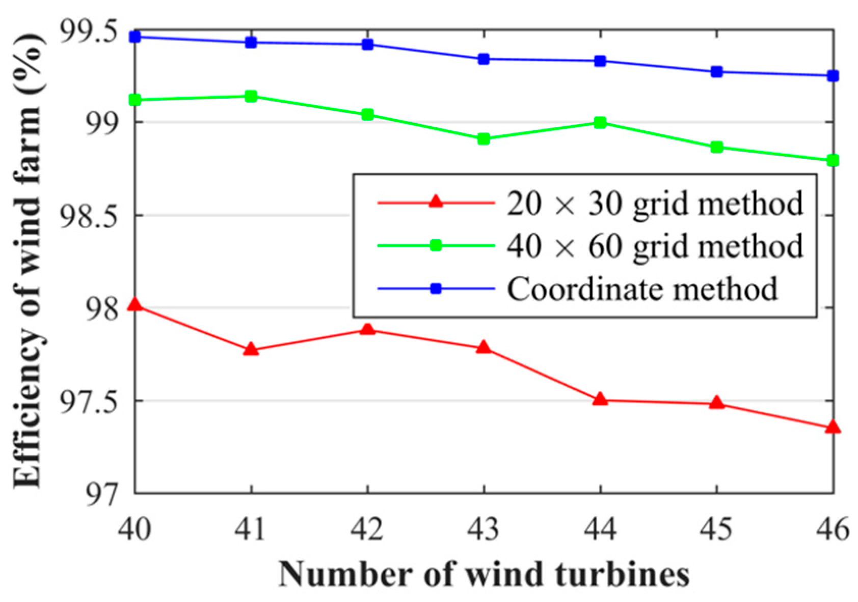
4.1. Comparison of Computational Results

Figure 4 shows the comparative results of cost of energy using the 20 × 30 grid method, 40 × 60 grid method, and coordinate method for the wind farm layout optimization. Various numbers of wind turbines from 40 to 46 are studied in this paper. As can be seen, there is a large improvement in the cost of energy for the 40 × 60 grid method and coordinate method when compared with the 20 × 30 grid method. The discrepancy between the 20 × 30 grid method and coordinate method can be up to 0.19 million dollars per megawatt when there are 46 wind turbines, while the 40 × 60 grid method yields a slightly larger cost of energy than the coordinate method. As the number of wind turbines increases, at a certain number of wind turbines there may be some fluctuations of the cost of energy (especially for the two grid methods), which is possibly because the sub-optimal results are obtained. In general, the cost of energy increases for all of the wind farm design methods as the number of wind turbines increases. According to the cost of energy results, it is concluded that the coarse 20 × 30 grid method is not sufficient for wind farm layout optimization, as it yields significantly inferior results when compared to other methods. In comparison, the results of the refined 40 × 60 grid method and coordinate method are much closer. In addition, the performance of the coordinate method is particularly stable, showing steadily increasing cost of energy with more turbines installed.

The comparative results of wind farm efficiency are presented in Figure 5 using different design methods for the number of wind turbines between 40 and 46. The wind farm efficiency is defined as the real wind farm power output when considering the wake losses divided by the theoretical wind farm power output neglecting the wake losses:

$$\mathrm{Wind}\mathrm{fam}\mathrm{efficiency}=\raisebox{1ex}{$P_{tot}\left(\mathrm{wake}\mathrm{losses}\right)$}\!\left/ \!\raisebox{-1ex}{$P_{tot}\left(\mathrm{wake}\mathrm{losses}\mathrm{neglected}\right)$}\right.$$

(21)

as can be seen from Figure 5, the trend of variation of wind farm efficiency is opposite to the cost of energy. When the number of wind turbines increases, the wind farm efficiency decreases. The decrease of wind farm efficiency for the 20 × 30 grid is the most prominent as compared to the other two methods. The maximum discrepancy of wind farm efficiency between the 20 × 30 grid method and coordinate method is 2% with 46 wind turbines. When applying the coordinate method, the wind farm efficiency is able to maintain above 99% for all different numbers of wind turbines, while the wind farm efficiency for the 40 × 60 grid is slightly smaller and fluctuating from approximately 99.1% to 98.8% as the number of wind turbines increases.

The total wind farm power outputs that were obtained by different wind farm design methods are presented in Figure 6 for different wind turbine numbers. Evidently, 20 × 30 grid method yields the lowest power output, which is approximately 200 kW less than the other two methods. The difference between the produced power predicted by the 40 × 60 grid method and the coordinate method are small. In general, the total power output linearly increases with the wind turbine number.

Table 4. Total wind farm power output increase of different number of wind turbines using refined 40 × 60 grid method and coordinate method with respect to the coarse 20 × 30 grid density.

Number of Turbines	40	41	42	43	44	45	46
Relative power increase using (40 × 60 grid)	1.13%	1.4%	1.19%	1.16%	1.53%	1.42%	1.49%
Relative power increase using coordinate method	1.47%	1.69%	1.58%	1.6%	1.87%	1.84%	1.96%

shows the variation in the wind farm power output predicted by the 40 × 60 grid method and the coordinate method relative to the 20 × 30 grid method. As the wind turbine number increases from 40 to 46, the power increase by using the 40 × 60 grid method varies roughly from 1% to 1.5%, while the power increase by using the coordinate method varies from 1.5% to 2%, depending on the number of installed wind turbines.

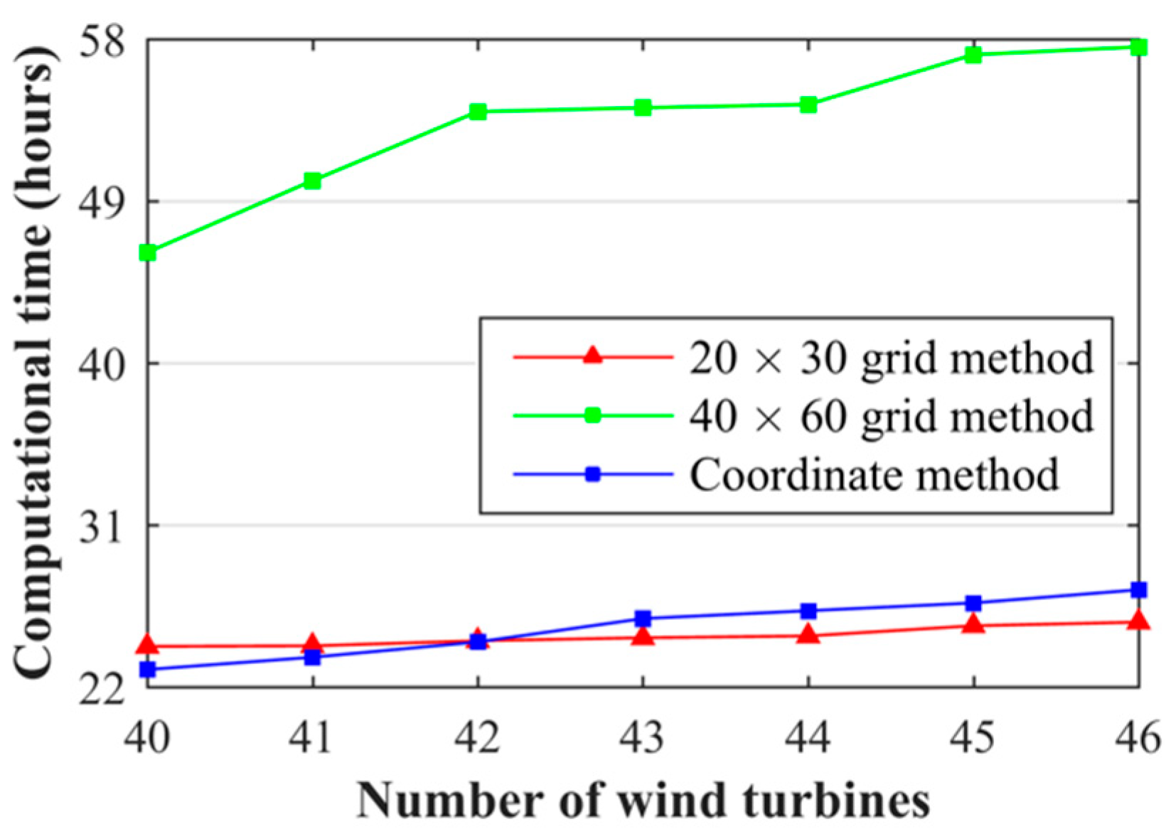
4.2. Comparison of Computational Cost

The computational costs of the optimization are quantified while using the wall time of High Performance Computer (HPC) that was running to more systematically compare the effectiveness of the methods. The computation is conducted using two 64-bit Intel Xeon Cores and 2 Gigabytes memory running on SUSE Linux operating system, and the codes are compiled with the Intel compiler. Figure 7 shows the running time of 20 × 30, 40 × 60, and the coordinate method for a different number of wind turbines. From the results, it is found that the 40 × 60 grid method consumes much more (almost two- or three-fold) computational time than the other two methods. In comparison, the increase of computational time with the coordinate method is faster than that with the 20 × 30 grid method. When there are less wind turbines, the 20 × 30 grid method consumes slightly more time than the coordinate method. When the number of wind turbines further increases, the coordinate method consumes more time.

4.3. Comparison of Optimal Wind Farm Layouts

Figure 8 shows the optimal layouts of 40 wind turbines, in which the wind turbine positions are indicated by the red-color cross symbols. The dominant wind directions are from the bottom to the top. In comparison, the layout for the 20 × 30 grid method is very different from the layouts that were obtained by the other two methods. The layouts for the 40 × 60 grid method and coordinate method are similar, which can be anticipated, since their optimization results are close to each other. In general, as many wind turbines as possible are distributed along the wind farm boundary to fully enlarge the distance between wind turbines. For the grid method, the wind turbine positions must be aligned with horizontal or vertical lines, which have limited feasible locations. For the coordinate method, their positions are more flexible and have no limits on the placement of wind turbines. With 46 wind turbines installed (shown in Figure 9), more wind turbines are located close to the wind farm boundary with the coordinate method, and those wind turbines present the staggered distribution pattern inside the wind farm area.

4.4. Angular Resolution Analysis of Wind Climatology

In order to consider the effect of angular resolution of wind climatology on the power output estimation and to compare the optimization results with a different wind farm design method in a more systematic and convincing way, the obtained optimal wind farm layouts with the setting of $15°$ wind direction division are they further evaluated with a finer $3°$ angular resolution. The comparative results with different wind farm design methods are shown in

Table 5. Comparison of the optimized total wind farm power output (in kW) with different wind farm design methods in a finer $3°$ angular resolution of wind climatology.

	Turbine Number	40	41	42	43	44	45	46
Design Methods
Grid method (20 × 30 grid)		8303	8484.4	8708.2	8899.5	9089.5	9274.2	9482.8
Grid method (40 × 60 grid)		8316.1	8504.9	8719.2	8924.1	9132.9	9302.3	9528.4
Coordinate method		8316.8	8534.5	8745.3	8924.6	9155.5	9345.6	9528.9

. As can be seen, when the finer wind direction division is applied for power output evaluation, the discrepancy of optimized total wind farm power output becomes even smaller and the power output of the densified 40 × 60 grid method and the coordinate method are very close to each other. Nevertheless, the coordinate method still yields slightly more power than the 40 × 60 grid method, followed by the 20 × 30 grid method. Quantitatively, when a finer angular resolution is applied for power output evaluation, the performance of wind farm layout optimization decreases from approximately 1.5% to 0.5%. Furthermore, by comparing the power output results with the original 15° and a finer 3° angular resolutions, it is found that the overall power output decrease is approximately 0.1%~0.3%, depending on the number of wind turbines optimized.

5. Conclusions

For planning/designing a wind farm, the layout optimization is an important step to be implemented in order to increase the profit return of wind farm project by alleviating the wake effect. In this paper, an irregular wind farm layout optimization is carried out with different layout design methods, including the discrete grid method and the continuous coordinate method. For the grid method, two grid densities of 20 × 30 and 40 × 60 are investigated to verify the performance of the method with the cell refinement. Techniques of handling the irregular boundary with different wind farm design methods are proposed to guarantee the feasible results of wind turbine placement. The optimization results show that the performance of a coarse 20 × 30 grid method is the worst, with a large cost of energy and low wind farm efficiency, but the computational cost is lower. By applying the densified grid cells, the grid method achieves a significant increase of total wind farm power output, varying from 1% to 1.5%, with 40 to 46 wind turbines being installed. However, the better optimization results can be achieved at the expense of significantly more computational time (roughly two- to three-fold more time than the coarse girds). In comparison, the coordinate method has the best performance in achieving the largest total wind farm power output. The relative increase of the total wind farm power output with the coordinate method is between 1.5% and 2% for 40 to 46 installed wind turbines with respect to the 20 × 30 grid method. The computational time of the coordinate method and the 20 × 30 grid method is the least and they are very close to each other. In conclusion, the coordinate method is the best option amongst the wind farm design methods, with a good balance of the wind farm optimization results and computational cost. By further evaluating the wind farm power output with the original $15°$ and finer $3°$ angular resolutions, it is found that the overall power output decrease is approximately 0.1%~0.3%, depending on the number of wind turbines optimized.

References

1. Lansdorp, B.; Williams, P. The Laddermill-Innovative Wind Energy from High Altitudes in Holland and Australia. Wind Power 2006, 6, 1–14. [Google Scholar]
2. Alotto, P.; Guarnieri, M.; Moro, F. Redox flow batteries for the storage of renewable energy: A review. Renew. Sustain. Energy Rev. 2014, 29, 325–335. [Google Scholar] [CrossRef]
3. Blaabjerg, F. Future on Power Electronics for Wind Turbine Systems. IEEE J. Emerg. Sel. Top. Power Electron. 2013, 1, 139–152. [Google Scholar] [CrossRef]
4. Van der Laan, M.P.; Hansen, K.S.; Sørensen, N.N.; Réthoré, P.-E. Predicting wind farm wake interaction with RANS: An investigation of the Coriolis force. J. Phys. Conf. Ser. 2015, 625, 012026. [Google Scholar] [CrossRef]
5. Nikolić, V.; Shamshirband, S.; Petković, D.; Mohammadi, K.; Cojbašić, Ž.; Altameem, T.A.; Gani, A. Wind wake influence estimation on energy production of wind farm by adaptive neuro-fuzzy methodology. Energy 2015, 80, 361–372. [Google Scholar] [CrossRef]
6. Shakoor, R.; Hassan, M.Y.; Raheem, A.; Wu, Y.K. Wake effect modeling: A review of wind farm layout optimization using Jensen’s model. Renew. Sustain. Energy Rev. 2016, 58, 1048–1059. [Google Scholar] [CrossRef]
7. Mosetti, G.; Poloni, C.; Diviacco, D. Optimization of wind turbine positioning in large wind farms by means of a Genetic algorithm. J. Wind Eng. Ind. Aerodyn. 1994, 51, 105–116. [Google Scholar] [CrossRef]
8. Beyer, H.G.; Rüger, T.; Schäfer, G.; Waldl, H.-P. Optimization of Wind Farm Configurations with Variable Number of Turbines. In Proceedings of the European Union Wind Energy Conference, Göteborg, Sweden, 20–24 May 1996; pp. 1073–1076. [Google Scholar]
9. Pérez, B.; Mínguez, R.; Guanche, R. Offshore wind farm layout optimization using mathematical programming techniques. Renew. Energy 2013, 53, 389–399. [Google Scholar] [CrossRef]
10. Feng, J.; Shen, W.Z. Solving the wind farm layout optimization problem using random search algorithm. Renew. Energy 2015, 78, 182–192. [Google Scholar] [CrossRef]
11. Chen, Y.; Li, H.; He, B.; Wang, P.; Jin, K. Multi-objective genetic algorithm based innovative wind farm layout optimization method. Energy Convers. Manag. 2015, 105, 1318–1327. [Google Scholar] [CrossRef]
12. Zhang, P.Y.; Romero, D.A.; Beck, J.C.; Amon, C.H. Solving wind farm layout optimization with mixed integer programs and constraint programs. EURO J. Comput. Optim. 2014, 2, 195–219. [Google Scholar] [CrossRef] [Green Version]
13. Wang, L.; Tan, A.C.C.; Gu, Y.; Yuan, J. A new constraint handling method for wind farm layout optimization with lands owned by different owners. Renew. Energy 2015, 83, 151–161. [Google Scholar] [CrossRef]
14. Wang, L.; Tan, A.C.C.; Cholette, M.E.; Gu, Y. Optimization of wind farm layout with complex land divisions. Renew. Energy 2017, 105, 30–40. [Google Scholar] [CrossRef]
15. Kuo, J.Y.J.; Romero, D.A.; Amon, C.H. A mechanistic semi-empirical wake interaction model for wind farm layout optimization. Energy 2015, 93, 2157–2165. [Google Scholar] [CrossRef]
16. Shakoor, R.; Hassan, M.Y.; Raheem, A.; Rasheed, N. Wind farm layout optimization using area dimensions and definite point selection techniques. Renew. Energy 2016, 88, 154–163. [Google Scholar] [CrossRef]
17. Wang, F.; Liu, D.; Zeng, L. Study on computational grids in placement of wind turbines using genetic algorithm. In Proceedings of the WNWEC 2009—2009 World Non-Grid-Connected Wind Power and Energy Conference, Nanjing, China, 24–26 September 2009; Volume 2, pp. 369–372. [Google Scholar]
18. Mittal, A. Optimization of the Layout of Large Wind Farms Using a Genetic Algorithm; Case Western Reserve University: Cleveland, OH, USA, 2010. [Google Scholar]
19. Wang, L.; Tan, A.C.C.; Gu, Y. Comparative study on optimizing the wind farm layout using different design methods and cost models. J. Wind Eng. Ind. Aerodyn. 2015, 146, 1–10. [Google Scholar] [CrossRef] [Green Version]
20. Engineering Model (OffWindEng). Available online: http://offwind.eu/Help/EngWindSim (accessed on 2 September 2017).
21. Jensen, N.O.O. A Note on Wind Generator Interaction; Risø National Laboratory: Roskilde, Denmark, November 1983; ISBN 87-550-0971-9. [Google Scholar]
22. Pookpunt, S.; Ongsakul, W. Optimal placement of wind turbines within wind farm using binary particle swarm optimization with time-varying acceleration coefficients. Renew. Energy 2013, 55, 266–276. [Google Scholar] [CrossRef]
23. Wang, L.; Cholette, M.E.; Tan, A.C.C.; Gu, Y. A computationally-efficient layout optimization method for real wind farms considering altitude variations. Energy 2017, 132, 147–159. [Google Scholar] [CrossRef]
24. Salcedo-Sanz, S.; Gallo-Marazuela, D.; Pastor-Sánchez, A.; Carro-Calvo, L.; Portilla-Figueras, A.; Prieto, L. Evolutionary computation approaches for real offshore wind farm layout: A case study in northern Europe. Expert Syst. Appl. 2013, 40, 6292–6297. [Google Scholar] [CrossRef]
25. Kusiak, A.; Song, Z. Design of wind farm layout for maximum wind energy capture. Renew. Energy 2010, 35, 685–694. [Google Scholar] [CrossRef]
26. Gebraad, P.; Thomas, J.J.; Ning, A.; Fleming, P.; Katherine, D. Maximization of the annual energy production of wind power plants by optimization of layout and yaw-based wake control. Wind Energy 2017, 20, 96–107. [Google Scholar] [CrossRef]
27. DuPont, B.; Cagan, J.; Moriarty, P. An advanced modeling system for optimization of wind farm layout and wind turbine sizing using a multi-level extended pattern search algorithm. Energy 2016, 106, 802–814. [Google Scholar] [CrossRef] [Green Version]
28. Abdulrahman, M.; Wood, D. Investigating the Power-COE trade-off for wind farm layout optimization considering commercial turbine selection and hub height variation. Renew. Energy 2017, 102, 267–278. [Google Scholar] [CrossRef]
29. Chen, Y. Commercial Wind Farm Layout Design and Optimization; Texas A&M University: College Station, TX, USA, 2013. [Google Scholar]
30. Zhang, C.; Hou, G.; Wang, J. A fast algorithm based on the submodular property for optimization of wind turbine positioning. Renew. Energy 2011, 36, 2951–2958. [Google Scholar]
31. Mikkelsen, R. Actuator Disc Methods Applied to Wind Turbines; Technical University of Denmark: Lyngby, Denmark, 2003. [Google Scholar]
32. Seguro, J.V.; Lambert, T.W. Modern estimation of the parameters of the Weibull wind speed distribution for wind energy analysis. J. Wind Eng. Ind. Aerodyn. 2000, 85, 75–84. [Google Scholar] [CrossRef]
33. Feng, J.; Shen, W.Z. Modelling wind for wind farm layout optimization using joint distribution of wind speed and wind direction. Energies 2015, 8, 3075–3092. [Google Scholar] [CrossRef]
34. Kirchner-Bossi, N.; Porté-Agel, F. Realistic Wind Farm Layout Optimization through Genetic Algorithms Using a Gaussian Wake Model. Energies 2018, 11, 3268. [Google Scholar] [CrossRef]
35. Eroglu, Y.; Seckiner, S.U. Design of wind farm layout using ant colony algorithm. Renew. Energy 2012, 44, 53–62. [Google Scholar] [CrossRef]
36. Lind, P.G.; Herráez, I.; Wächter, M.; Peinke, J. Fatigue Load Estimation through a Simple Stochastic Model. Energies 2014, 7, 8279–8293. [Google Scholar] [CrossRef] [Green Version]
37. Abdelsalam, A.M.; El-Shorbagy, M.A. Optimization of wind turbines siting in a wind farm using genetic algorithm based local search. Renew. Energy 2018, 123, 748–755. [Google Scholar] [CrossRef]
Figure 1. PARK wake model.
Applsci 09 00639 g001
Figure 2. Schematic of the boundary handling technique for the optimization study using the grid method with: (a) coarse 20 × 30 grid and (b) refined 40 × 60 grid.
Applsci 09 00639 g002
Figure 3. Schematic of the boundary handling technique for the optimization using the coordinate method.
Applsci 09 00639 g003
Figure 4. Wind farm cost of energy results (in million dollars per megawatt) for different design methods.
Applsci 09 00639 g004
Figure 5. Wind farm efficiency results for different design methods.
Applsci 09 00639 g005
Figure 6. Total wind farm power for different design methods.
Applsci 09 00639 g006
Figure 7. Computational time of different design methods for different wind turbine numbers.
Applsci 09 00639 g007
Figure 8. Comparison of optimal wind farm layouts of 40 turbines by: (a) 20 × 30 grid method, (b) 40 × 60 grid method, and (c) coordinate method.
Applsci 09 00639 g008
Figure 9. Comparison of optimal wind farm layouts of 46 turbines by: (a) 20 × 30 grid method, (b) 40 × 60 grid method, and (c) coordinate method.
Applsci 09 00639 g009