Posture Stabilization of Wheeled Mobile Robot Based on Passivity-Based Robust Switching Control with Model Uncertainty Compensation

Abstract

This study presents apassivity-based robust switching control for the posture stabilization of wheeled mobile robots (WMRs) with model uncertainty. Essentially, this proposed strategy is switching between (1) passivity-based robust control to lead the robot to the neighborhood of local minima with a finite time and (2) another robust control to perturb the w-rotational motion of the WMR before the v-kinetic energy of the WMR become meaningless, thereby, eventually converging to the desired posture. Thus, combining two switching control laws ensures the global convergence of (x,y)-navigation of WMRs from any initial position to desired set. Especially, the inter-switching time is intentionally selected before the WMR completely loses its mobility, which ensures a strict decrease in (x,y)-navigation potential energy and a better global convergence rate. In addition, this control architecture also includes model uncertainty compensation, often neglected in practice, and analytical study of rotational perturbation was also conducted. The Lyapunov technique and energetic passivity were utilized to derive this control law. Simulation results are presented to illustrate the effectiveness of the proposed technique. It was found from the results that the WMR was quickly converged to the desired posture even under the presence of model uncertainty.

1. Introduction

Wheeled mobile robots (WMRs) play a central role in practice such as material handling [1], space exploration [2], and smart wheel chairs [3], as well as, mobile sensor networks [4]. Moreover, the WMR is also known for a theoretically rich dynamical system because of the presence of non-holonomic constraints [5] (i.e., no-slip conditions).

The concept of passivity has emerged as very powerful tool for many control problems in robotics: general motion control and teleportation [6,7], biped walking robots [8], and multi-robot cooperative control [9,10]. Numerous feedback control approaches have been studied for the posture stabilization of WMRs. (e.g., [11,12,13,14,15,16,17,18,19]). Especially, a control law based upon passivity concept has been proposed [20] but the complicated canonical transformation was required with solving the non-trivial partial differential equation. Recently, the passivity-based Lyapunov-based stabilization control of the differential mobile robot with assistance of an extended Kalman filter was investigated [21] and an integral sliding mode control for the trajectory tracking of wheeled mobile robots was proposed [22]. Furthermore, regarding robust control, the Sliding Mode based robust control application to the second order nonlinear robot manipulator system have also been described ([23,24]).

Works based upon the first order kinematic model of WMRs (or unicycles) [14,15,16,20,21,22] are not applicable for a system where the inertia effect of the robot is sufficient to affect the performance of a given task. However, in [19], the novel framework was successfully addressed for this issue without any transformation, directly utilizing the second order dynamics of WMR. Specifically, [19] proposeda passivity-based switching control, which made the WMR move back and forth between two switching manifolds in such a way that a certain posture-specifying potential function was monotonically decreasing. This control law allows us to initiate switching even before reaching each of the (zero-measure) switching manifolds with zero velocity, convergence to which takes, in theory, an infinitely long time. Yet, for doing so, it requires perfect cancellation of Coriolis terms, which may not be effective and feasible in reality. Moreover, constructing the switching manifolds is required. Due to those motivations, a passivity-based robust switching control for the posture stabilization of wheeled mobile robots with model uncertainty (i.e., inertia effect) compensation is presented without the use of any complicated transformations [18] and other accessories (for an instance, switching manifolds [19]) in this study. Therefore, this approach is more practical and convenient to implement than [18] using the complicated canonical transformation and [19] requiring perfect cancellation of Coriolis effect along with switching manifolds. Also, like [19], the control law is designed based upon the second order Lagrangian (v,w)-WMR dynamics which are more intuitive and convincing than the first order kinematics based approaches [14,15,16,20,21,22]). Although the adaptive and robust control-based first order approaches have been thoroughly studied in the literature, the second order Lagrangian (v,w)-WMR dynamics based robust control for model uncertainty has not been fully investigated. In addition, this control scheme allows the WMR to continuously move in the forward/backward direction by reducing the navigation potential energy while at the same time gaining perturbation energy without stopping at a certain (x,y) position compared to [19]. Besides, this work includes the analysis of the perturbation angle for the WMR to proceed further navigation and avoid unwanted local minima.

The strategy of control switches between two control modes: (1) passivity-based robust control to the neighborhood of local minima with a finite time and (2) another robust control to perturb for regaining further navigation potential energy before the forward velocity-based kinetic energy perfectly becomes zero, so that they eventually converge to desired posture with any defined error bound. Thus, this law of combining switching control modes ensures the global convergence of (x,y)-navigation from any initial position to a defined desired set while compensating model uncertainty and ensuring a finite control time for each control between switches. The rest of paper is as follows: The dynamics of WMRs is given and reviewed in Section 2 and the proposed control law is designed and analyzed in Section 3. Simulation results are presented in Section 4. The concluding remarks are stated in Section 5.

2. SecondOrder Dynamics of Wheeled Mobile Robots

Consider the following 3-DOF $(x,y,\theta )$ wheeled mobile robot, as shown in Figure 1, which consists of two independently controlled rear wheels and a front passive caster to avoid rolling over.

Its dynamics is given by Lee at al. [19],

$$M(\theta )\dot{\mathsf{\upsilon }}+C(\theta ,\dot{\theta })\mathsf{\upsilon }=u$$

(1)

where $\mathsf{\upsilon }={\left[\begin{array}{cc}v& w\end{array}\right]}^{{\rm T}}\in {\mathsf{\Re }}^2$ is the forward velocity and angular velocity of the robot, $u={[\begin{array}{cc}{u}_v& u_w\end{array}]}^{{\rm T}}\in {\mathsf{\Re }}^2$ is the control force, $M(\theta )\in {\mathsf{\Re }}^{2\times 2}$ is an inertia symmetric positive definitive matrix, and $C(\theta ,\dot{\theta })\in {\mathsf{\Re }}^{2\times 2}$ is a Coriolis matrix which satisfy $\dot{M}(\theta )-2C(\theta ,\dot{\theta })=-{[\dot{M}(\theta )-2C(\theta ,\dot{\theta })]}^T$. This skew-symmetric property implies that the WMR (wheeled mobile robot) holds energetic passivity property [19].

Specifically, the dynamics is given by

$$\left[\begin{array}{cc}m& 0\\ 0& I_r\end{array}\right]\left[\begin{array}{c}\dot{v}\\ \dot{w}\end{array}\right]+\left[\begin{array}{cc}0& -md\dot{\theta }\\ md\dot{\theta }& 0\end{array}\right]\left[\begin{array}{c}v\\ w\end{array}\right]=\left[\begin{array}{c}{u}_v\\ u_w\end{array}\right]$$

(2)

where $d\ge 0$ is the distance between $(x_c,y_c)$ and $(x_o,y_o)$; $m$ and $I_r=m{d}^2+I_c$ are a mass of WMR and an inertia of the robot with respect to $(x_o,y_o)$ respectively; $I_c$ is the inertia with respect to, $(x_c,y_c)$; $u_v=\frac{1}{r}({\tau }_r+{\tau }_l)$ and $u_w=\frac{c}{r}({\tau }_r-{\tau }_l)$, where ${\tau }_r$,${\tau }_l$ $\in \mathsf{\Re }$ are the right and left torques conveyed by independent actuators; and $r$ and $c$ are the radius of wheel and the half width of the robot.

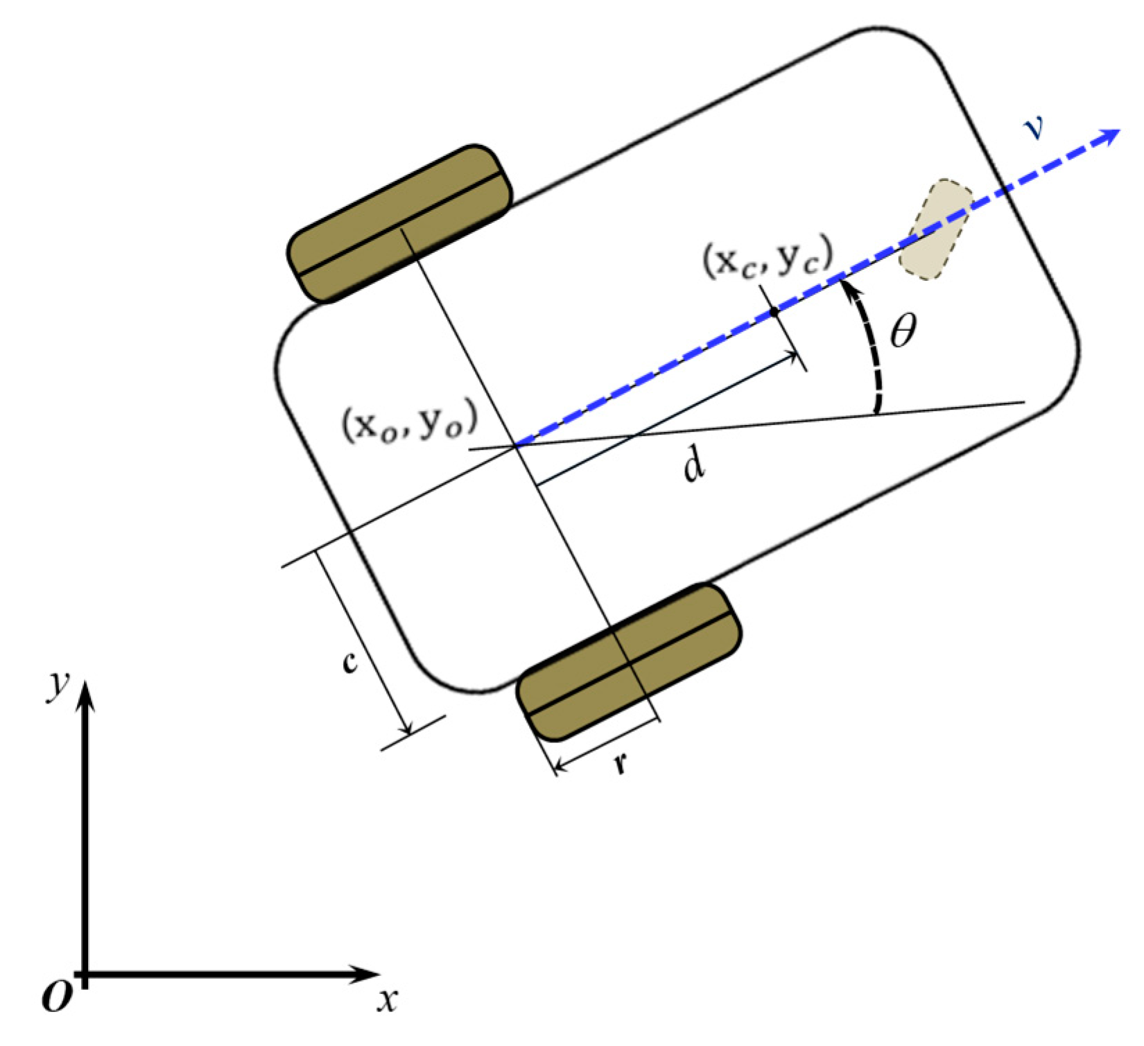
3. Passivity Based Robust Switching Control Design for Posture Stabilization

The primary purpose of control law is to cause the robot to move from any initial position $(x_i,y_i)\in {\mathsf{\Re }}^2$ to the desired set of position such as

$$E_d:=\{x_d,y_d\in \mathsf{\Re }| dist(x(t) y(t), x_d y_d)\le B\}$$

(3)

where B$\in \mathsf{\Re }$ is the positive bounded real number which can be determined by the specific performance error bound. Additionally, the orientation of the robot should reach the desired angle ($\theta$) such that $\theta \to {\theta }_d\in \mathsf{\Re }$. In this paper, without losing generality, we assume the desired position and orientation as $(x_d,y_d,{\theta }_d)=(0,0,0)$.

Next, in order to construct the passivity-based switching control, let’s consider the following total energy of the robot system as the Lyapunov function,

$$L_t(t)=L_v(t)+L_w(t)={\kappa }_v(t)+{\phi }_v(x,y)+{\kappa }_w(t)+{\phi }_w(\theta )$$

(4)

where $L_t(t)$ $\in \mathsf{\Re }$ is the total energy; $L_v(t)={\kappa }_v(t)+{\phi }_v(t)$ and $L_w(t)={\kappa }_w(t)+{\phi }_w(t)$ where ${\kappa }_v(t)$ and ${\kappa }_w(t)$ are forward motion and rotational kinetic energies, and ${\phi }_v(t)$ and ${\phi }_w(t)$ area (x,y)-navigation energy and an orientation potential energy, respectively. In particular, the kinetic energies can be defined as ${\kappa }_v(t)=1/2 mv{(t)}^2$ and ${\kappa }_w(t)=1/2 I_{r}w{(t)}^2$.

Remark 1.

(Properties of potential energy) Functions${\phi }_v(x,y)\ge 0$(${\phi }_v:{\mathsf{\Re }}^2\to \mathsf{\Re }$) and${\phi }_w(\theta )\ge 0$(${\phi }_v:\mathsf{\Re }\to \mathsf{\Re }$) are the (x,y)-navigation potential function and$\theta$-orientation potential function respectively. These functions satisfy the following properties: (1)${\phi }_v(x,y)=0\iff$$(x,y)=0$and (2)$(\frac{\partial {\phi }_v(x,y)}{\partial x},\frac{\partial {\phi }_v(x,y)}{\partial y})=0$$\iff$$(x,y)=0$. Similarly, for the$\theta$-potential function${\phi }_w(\theta )$,${\phi }_w(0)=0$and$\frac{\partial {\phi }_w(\theta )}{\partial \theta }=0$$\iff$$\theta =0$[19,25].

For this study, let’s define the following potential energies such that ${\phi }_v(x,y)=\frac{1}{2}(K_x{x}^2+K_y{y}^2)$ for the target position of WMR as the origin of (x,y)-plane and ${\phi }_v(\theta )=\frac{1}{2}{K}_{\theta }{\theta }^2$ for the desired orientation as 0, satisfying Remark 1, and where $K_x$, $K_y$, and $K_{\theta }$ $\in \mathsf{\Re }$ are the positive coefficients.

Furthermore, taking derivative of Equation (3) with respect to a time yield,

$${\dot{L}}_t(t)={\dot{\kappa }}_v(t)+\frac{\partial {\phi }_v(x,y)}{\partial x}\frac{dx}{dt}+\frac{\partial {\phi }_v(x,y)}{\partial y}\frac{dy}{dt}+{\dot{\kappa }}_w(t)+\frac{\partial {\phi }_w(\theta )}{\partial \theta }\frac{d\theta }{dt}$$

(5)

By the admissible (i.e., not violating the non-holonomic constraints [5,19]) velocity of WMRs, we have $\dot{x}=v\cos \theta$ and $\dot{y}=v\sin \theta$. Thus,

$${\dot{L}}_t(t)={\dot{\kappa }}_v(t)+\frac{\partial {\phi }_v(x,y)}{\partial x}v\cos \theta +\frac{\partial {\phi }_v(x,y)}{\partial y}v\sin \theta +{\dot{\kappa }}_w(t)+\frac{\partial {\phi }_w(\theta )}{\partial \theta }w$$

(6)

Here, the total energy can be decomposed into ${\dot{L}}_v(t)$ and ${\dot{L}}_w(t)$,

$${\dot{L}}_v(t)=v\left[m\dot{v}+\frac{\partial {\phi }_v(x,y)}{\partial x}\cos \theta +\frac{\partial {\phi }_v(x,y)}{\partial y}\sin \theta \right]$$

(7)

$${\dot{L}}_{\dot{\theta }}(t)=w\left[I_r \dot{w}+\frac{\partial {\phi }_w(\theta )}{\partial \theta }\right]$$

(8)

Substituting Equation (2) into Equations (7) and (8) yields

$${\dot{L}}_v(t)=v\left[md{w}^2+u_v+\frac{\partial {\phi }_v(x,y)}{\partial x}\cos \theta +\frac{\partial {\phi }_v(x,y)}{\partial y}\sin \theta \right]$$

(9)

$${\dot{L}}_w(t)=w\left[-mdw v+u_w+\frac{\partial {\phi }_w(\theta )}{\partial \theta }\right]$$

(10)

To ensure the negative semi-definitive of Equations (9) and (10) individually, we can suggest the following control law,

$$\left[\begin{array}{c}{u}_v\\ u_w\end{array}\right]=\left[\begin{array}{c}-md w^2\\ md w v\end{array}\right]-\left[\begin{array}{c}\frac{\partial {\phi }_v(x,y)}{\partial x}\cos \theta +\frac{\partial {\phi }_v(x,y)}{\partial y}\sin \theta +\alpha sat(\frac{v}{\Phi })\\ \frac{\partial {\phi }_{\dot{\theta }}(\theta )}{\partial \theta }+\beta w\end{array}\right]$$

(11)

where $sat (v/\Phi )=sign (v/\Phi )$ if $\left|v\right|>\Phi$ and $sat (v/\Phi )=v/\Phi$ if $\left|v\right|\le \Phi$ is the positive boundary layer thickness to eliminate the chattering on the sliding phase [26] and $\alpha$ and $\beta \in \mathsf{\Re }$ are the positive constant gains. The control law, Equation (11), ensures both ${\dot{L}}_v(t)=-\alpha v sat(v/\Phi )\le 0$ and ${\dot{L}}_w(t)=-\beta w^2\le 0$ and the derivative of the overall Lyapunov function is also ${\dot{L}}_t(t)=-\alpha v sat(v/\Phi )-\beta w^2\le 0$.

Remark 2.

(model uncertainty) The Coriolis terms of the control law Equation (11) contains$md$which is usually difficult to measure its exact value. In this regard, the model uncertainty should be considered to achieve better navigation performance of WMR in reality. In this study, we denote the estimation of$md$ as $\gamma$, and assume to know a bounded constant $\exists \rho \in \mathsf{\Re }$ s.t $\left|md-\gamma \right|\le \rho$.

Based on Equation (11), the control law including the compensation of the model uncertainty is then designed to be

$$\begin{gathered} \left[\begin{array}{c}{u}_v\\ u_w\end{array}\right]=\left[\begin{array}{c}{F}_v\\ F_w\end{array}\right]+\left[\begin{array}{c}-\frac{\partial {\phi }_v(x,y)}{\partial x}\cos \theta -\frac{\partial {\phi }_v(x,y)}{\partial y}\sin \theta -\alpha sat(\frac{v}{\Phi })\\ -\frac{\partial {\phi }_w(\theta )}{\partial \theta }-\beta w\end{array}\right] \\ {F}_v=\langle \begin{array}{cc}-\gamma w^2-\rho w^2 sign(\frac{v}{\Phi })\hspace{1em}& if \left|v\right|>\Phi \\ 0& if \left|v\right|\le \Phi \end{array} \mathrm{and} \\ {F}_w=\langle \begin{array}{cc}\gamma w v-\rho w v sign(\frac{v}{\Phi })\hspace{1em}& if \left|v\right|>\Phi \\ 0& if \left|v\right|\le \Phi \end{array} \end{gathered}$$

(12)

Here, the robot system is governed by two separate control laws according to $\left|v\right|>\Phi$ and $\left|v\right|\le \Phi$.

This control law Equation (12) ensures that ${\dot{L}}_v(t)\le 0$ and ${\dot{L}}_w(t)\le 0$ individually while compensating the model uncertainty of system out of boundary layer, $\Phi$. On the other hand, although we cannot individually ensure ${\dot{L}}_v(t)\le 0$ and ${\dot{L}}_w(t)\le 0$ within the boundary layer, we still have ${\dot{L}}_t(t)\le 0$. This is because if $\left|v\right|>\Phi$, applying (12) into Equations (9) and (10), it is found that,

$$\begin{gathered} {\dot{L}}_v(t)=\left[\left[md-\gamma \right]w^2-\rho w^{2}sign(\frac{v}{\Phi })-\alpha sign(\frac{v}{\Phi })\right]v\le -v\left[\alpha sign(\frac{v}{\Phi })\right]\le 0 \\ {\dot{L}}_w(t)=\left[\left[\gamma -md\right]v w-\rho v w sign(\frac{v}{\Phi })-\beta w\right]w\le -\beta w^2\le 0 \end{gathered}$$

(13)

Also, the closed-loop dynamics of WMR for $\left|v\right|>\Phi$ is given by,

$$\begin{gathered} m\dot{v}+\left[\gamma -md\right]w^2+\rho w^{2}sign(\frac{v}{\Phi })+\alpha sign(\frac{v}{\Phi })+\frac{\partial {\phi }_v(x,y)}{\partial x}\cos \theta +\frac{\partial {\phi }_v(x,y)}{\partial y}\sin \theta =0 \\ I\dot{w}+\left[md-\gamma \right]v w+\rho v w sign(\frac{v}{\Phi })+\beta w+\frac{\partial {\phi }_w(\theta )}{\partial \theta }=0 \end{gathered}$$

(14)

On the other hand, if $\left|v\right|\le \Phi$,

$$\begin{gathered} {\dot{L}}_t(t)={\dot{L}}_v(t)+{\dot{L}}_w(t)\le 0 \mathrm{with} {\dot{L}}_v(t)=\left[-md{w}^2-\alpha \frac{v}{\Phi }\right]v \mathrm{and} \\ {\dot{L}}_w(t)=\left[mdv w-\beta w\right]w \end{gathered}$$

(15)

The corresponding closed-loop dynamics of the WMR is given by,

$$\begin{gathered} m\dot{v}-md{w}^2+\alpha \frac{v}{\Phi }+\frac{\partial {\phi }_v(x,y)}{\partial x}\cos \theta +\frac{\partial {\phi }_v(x,y)}{\partial y}\sin \theta =0 \\ I\dot{w}+mdv w+\beta w+\frac{\partial {\phi }_w(\theta )}{\partial \theta }=0 \end{gathered}$$

(16)

Proposition 1.

(Decrease of (x,y)-navigation potential energy and finite control time) Under Equation (12), if the initial velocity of WMR is $\left|v(t_0)\right|\le \Phi$, the (x,y)-navigation potential energy of WMR is strictly decreased from $t_0$ to $t^{*}$ such that,

$${\phi }_v( t^{*} ) < {\phi }_v(t_0)$$

(17)

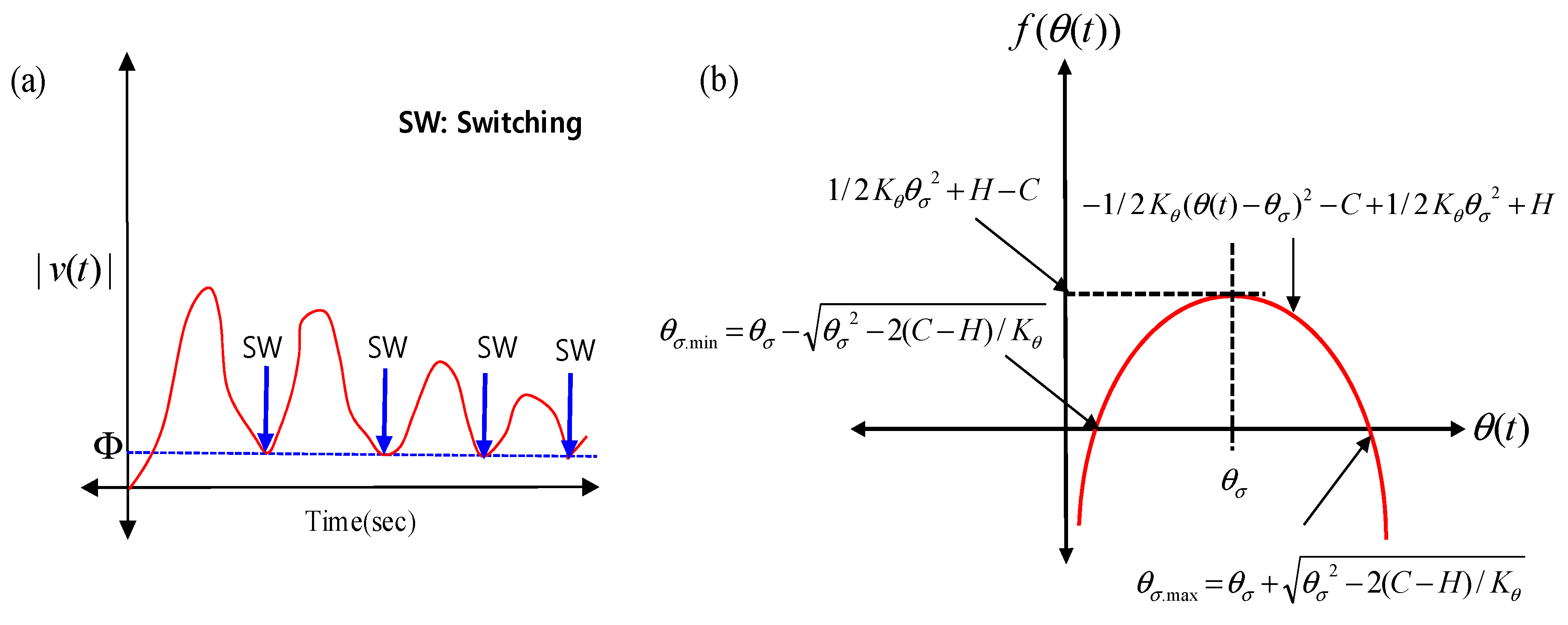
where $t^{*}$ is defined as another particular time when the perturbed v(t) meets this condition $\left|v(t^{*})\right|=\Phi$ for the first time. According to Equation (14), the WMR initiates its navigation by accelerating itself until losing its own kinetic energies thus the transient forward velocity |v(t)| is suddenly increased from $v(t_0)$ and eventually decreased to $\left|v(t^{*})\right|=\Phi$. In other words, we have such a scenario: $\left|v(t_0)\right|\to \left|v(t)\right|\to \left|v(t^{*})\right|=\Phi$ for $\forall t\in ( t_0\hspace{1em}{t}^{*})$ with $\left|v(t_0)\right|\le \left|v(t^{*})\right|<\left|v(t)\right|$ (see Figure 2a).

By investigating Equation (14), it is obvious based on the property of second order Lagrangian dynamics that the potential force and moment $\frac{\partial {\phi }_v(x,y)}{\partial x}\cos \theta +\frac{\partial {\phi }_v(x,y)}{\partial y}\sin \theta$ and $\frac{\partial {\phi }_w(\theta )}{\partial \theta }$ will perturb both v and w of WMR initially and eventually the perturbed v and w will be decreased by damping terms $\alpha sign(v/\Phi )$ and $\beta w$.

In addition, the control duration to enforce WMR to move from the initial position to the particular one with $\left|v\right|=\Phi$ is bounded by,

$$\Delta t<\frac{{\phi }_v(t_0)+0.5m{\Phi }^2}{\alpha \Phi }$$

(18)

where $\Delta t=t^{*}-t_0>0$ is the control duration. □

Proof :

From $t_0$ to $t^{*}$, the strict decrease of the potential energy will occur due to the following reasons: if $\left|v\right|>\Phi$, we know from Equation (13) that,

$${\dot{L}}_v(t)\le -v(t)\left[\alpha sign (\frac{v(t)}{\Phi })\right]=-\alpha \left|v(t)\right|<-\alpha \Phi \mathrm{for} \forall t\in [t_0 t^{*}]$$

(19)

Integrating Equation (19) from $t_0$ to $t^{*}$ yields,

$$L_v(t^{*})-L_v(t_0)<-\alpha \Phi \Delta t$$

(20)

Furthermore, Equation (20) implies that,

$${\phi }_v(t^{*})-{\phi }_v(t_0)<-\alpha \Phi \Delta t+{\kappa }_v(t_0)-{\kappa }_v(t^{*})\le -\alpha \Phi \Delta t<0\Rightarrow {\phi }_v(t^{*})<{\phi }_v(t_0)$$

(21)

Since ${\kappa }_v(t_0)-{\kappa }_v(t^{*})\le 0$ with ${\kappa }_v(t^{*})=0.5m {\Phi }^2$, ${\kappa }_v(t_0)=0.5m v{(t_0)}^2$ and a given condition $\left|v(t_0)\right|\le \Phi$. Therefore, Equation (17) is true.

Furthermore, Equation (20) can be extended into ${\phi }_v(t) < {\phi }_v(t_0)$ for $\forall t\in (t_0\hspace{1em}{t}^{*})$ due to the reason ${\kappa }_v(t_0)\le {\kappa }_v(t)$ for $\forall t\in (t_0\hspace{1em}{t}^{*})$. This is because we have a following transient scenario $\left|v(t_0)\right|\to \left|v(t)\right|\to \left|v(t^{*})\right|=\Phi$ for $\forall t\in ( t_0 t^{*})$ with $\left|v(t_0)\right|\le \left|v(t^{*})\right|<\left|v(t)\right|$ (see Figure 2a).

Also, Equation (18) is also true because,

$$L_v(t^{*})-L_v(t_0)<-\alpha \Phi \Delta t\Rightarrow \Delta t<\frac{L_v(t_0)-L_v(t^{*})}{\alpha \Phi }$$

(22)

Furthermore,

$$\Delta t<\frac{{\phi }_v(t_0)-{\phi }_v(t^{*})+k_v(t_0)-k_v(t^{*})}{\alpha \Phi }<\frac{{\phi }_v(t_0)+k_v(t_0)}{\alpha \Phi }\le \frac{{\phi }_v(t_0)+0.5m{\Phi }^2}{\alpha \Phi }$$

(23)

Consequently, $\Delta t$ is bounded by initial (x,y)-navigation potential energy and v-kinetic energy. Proof completed. □

Proposition 2.

(convergence) Under control law, Equation (12) for the domain $\left|v\right|\le \Phi$, the states $X=$ [x, y, v, w, $\theta$] $\in {\mathsf{\Re }}^5$ of the WMR converge to the following set. □

$$E_c:=\{X\in \mathsf{\Re }| \frac{\partial {\phi }_v(x,y)}{\partial x}\cos \theta +\frac{\partial {\phi }_v(x,y)}{\partial y}\sin \theta =0,(v,w,\theta )=(0,0,0)\}$$

(24)

Proof :

For $\left|v\right|\le \Phi$, we know that ${\dot{L}}_t(t)=-\alpha \frac{v^2}{\Phi }-\beta w^2\le 0$ (i.e., bounded) for $\forall X (t)\in \Omega$, where $\Omega : {\dot{L}}_t(X(t))\le 0$ is a compact set containing $X (t_o)$. Define $M:=\{X\in \Omega | {\dot{L}}_t(t)=0\}$. Let $E_c\in M\in \Omega$ be the largest invariant set in $M$. Since $X (t_0)\in \Omega$, $X (t)\to E_c$. Applying an invariant Theorem [27] with ${\dot{L}}_t(t)\le 0$ to (16) yields $(v,w,\theta )\to 0$ and $\frac{\partial {\phi }_v(x,y)}{\partial x}\cos \theta +\frac{\partial {\phi }_v(x,y)}{\partial y}\sin \theta \to 0$. □

Remark 3. 

There exist multiple solutions of$\frac{\partial {\phi }_v(x,y)}{\partial x}\cos \theta +\frac{\partial {\phi }_v(x,y)}{\partial y}\sin \theta =0$,

(1)

If$(x,y)=0$(This is what we desire to achieve.)

(2)

If$\frac{\partial {\phi }_v(x,y)}{\partial x}=0$,$\sin \theta =0$(i.e.,$\theta =\pm n\pi$for$\forall n\in {\rm Z}$), and$y\ne 0$.

(3)

If$\frac{\partial {\phi }_v(x,y)}{\partial y}=0$,$\cos \theta =0$(i.e.,$\theta =\pm \frac{n\pi }{2}$for$\forall n\in N$), and$x\ne 0$.

(4)

If$\tan \theta =-\frac{{\phi }_{v.x}(x,y)}{{\phi }_{v.y}(x,y)}$, where,${\phi }_{v.x}(x,y)=\frac{\partial {\phi }_v(x,y)}{\partial x}\ne 0$and${\phi }_{v.y}(x,y)=\frac{\partial {\phi }_v(x,y)}{\partial y}\ne 0$.

The first condition of Remark 3 is the desired position of robot. Thus, the given task is completed. Condition 3 implies that there exists a w-motion ($\theta \ne 0$) so that the w-dynamics (rotational motion) induces the v-dynamics ($v\ne 0$). Condition 4 induces both v and w dynamics ($x\ne 0$, $y\ne 0$, $\theta \ne 0$). Thus, both Equations (3) and (4) are not invariant which leads that the WMR is under the motion. For Condition 2, if both v and w are 0 with $\theta =0$ for n = 0, then closed-loop dynamics Equation (16) become $m_r\dot{v}=0$ and $I_r\dot{w}=0$. This implies that the robot will be stuck in the middle of y-axis (i.e., unwanted local minima).

According to Remark 3, we can define a set (unwanted) local minima where the robot should avoid or pass through s.t

$$E_{avoid}:=\{X\in \mathsf{\Re }| v=w=\theta =0,x=0,y\ne 0\}$$

(25)

By inspecting Equations (16) and (25), the WMR will begin to lose its own kinetic energies as it approaches $E_{avoid}$ and finally be trapped at $E_{avoid}$. Therefore, with an intuitive sense, we should not wait until robot is stuck at $E_{avoid}$ (i.e., unwanted local minima) and have to utilize another control at the non-zero forward velocity such as the condition $\left|v\right|=\Phi \ne 0$ for better navigation performance. This way possibly preserves current v-kinetic energies (at least $0.5 m {\Phi }^2$) for next switched control law. In this regard, the following switching law is presented to allow the robot to reach $E_d$.

Theorem 1.

(Robust switching control law) The following control law enables us to accomplish that the robot is able to pass through the forbidden region such as a set $E_{avoid}$ and then reach the final desired position s.t $E_d$. Based on Equation (12), the modified control laws are designed to be,

$$\left[\begin{array}{c}{u}_{v.1}\\ u_{w.1}\end{array}\right]:==\left[\begin{array}{c}{F}_v-\frac{\partial {\phi }_v(x,y)}{\partial x}\cos \theta -\frac{\partial {\phi }_v(x,y)}{\partial y}\sin \theta -\alpha sign(\frac{v}{\Phi })\\ F_w-K_1 w-K_{\theta }\theta \end{array}\right] hold until \left|v\right|\to \Phi$$

(26)

$$\left[\begin{array}{c}{u}_{v.2}\\ u_{w.2}\end{array}\right]:==\left[\begin{array}{c}{F}_v-\frac{\partial {\phi }_v(x,y)}{\partial x}\cos \theta -\frac{\partial {\phi }_v(x,y)}{\partial y}\sin \theta -\alpha sign(\frac{v}{\Phi })\\ F_w-K_{1}w-K_{\theta }(\theta -{\theta }_{\sigma })\end{array}\right] hold until \left|v\right|\to \Phi$$

(27)

where $K_v,K_1\in \mathsf{\Re }$ are the positive constant gains. Let $t_1, t_2,\cdots ,t_n\in [t_0\hspace{1em}{t}_f]$ be each switching time between the first control [$u_{v.1}$ $u_{w.1}$] and the second one [$u_{v.2}$ $u_{w.2}$] or vice versa at the moment $\left|v\right|=\Phi \ne 0$. If we assume that the initial states of the WMR do not belong to $E_{avoid}$, the first control law is initially activated to transport the robot until $\left|v\right|\to \Phi$, where the (x,y)-navigation potential energy is monotonically decreased according to Proposition 1. Simultaneously, $\theta \approx 0$ is possibly achieved via $-K_1 w-K_{\theta }\theta$ in Equation (26). If the WMR enters into $E_d$ via a pure action of [$u_{v.1}$ $u_{w.1}$] and then following control will be performed to ensure $\theta \to 0$.

$$\left[\begin{array}{c}{u}_v\\ u_w\end{array}\right]=\left[\begin{array}{c}-K_{v}v\\ -K_{1}w-K_{\theta }\theta \end{array}\right]\hspace{1em}hold until\hspace{1em}\theta \to 0$$

(28)

However, if the WMR is still outside of $E_d$, it will switch from the first control law to the second one until, again, $\left|v\right|\to \Phi$. The second law induces the rotational motion (i.e., $\theta \to {\theta }_a$) so that the forward velocity of WMR suddenly increases and, due to damping term $-\alpha sign(v/\Phi )$, decreases eventually. This is because the v-dynamics is coupled with the w-dynamics. Due to this perturbation invoking the forward velocity v(t), the (x,y)-navigation potential energy of WMR is also diminished. Therefore, either control in (24) strictly reduces the (x,y)-navigation potential energy so that the WMR finally reaches $E_d$ by conducting the switching back and forth between Equations (26) and (27). □

Proof :

Based on Proposition 1, if $\left|v(t_0)\right|\le \Phi$, the first control in Equation (26) guarantees the strict decrease of (x,y)-navigation potential energy until the time $t_1$ when $\left|v(t_1)\right|=\Phi$. In other words, ${\phi }_v(t) < {\phi }_v(t_0)$ for $\forall t\in [t_0\hspace{1em}{t}_1]$. If the WMR enters into $E_d$ via Equation (26), switch from Equation (26) to Equation (28) for correcting the orientation of the WMR (i.e., $\theta \to 0$). Based on the following Lyapunov function $L_t(t)=1/2m{v}^2+1/2I_r{w}^2+1/2K_{\theta }{\theta }^2$, applying Equation (28) into Equation (2) yields ${\dot{L}}_t(t)=-(K_v{v}^2+K_1 w^2)$. This implies that $\theta \to 0$. Therefore, the final correction of WMR orientation can be achieved via Equation (28).

However, if the WMR is still outside of $E_d$, the second control is initiated to gain a rotational energy for further navigation (i.e., $\theta \to {\theta }_a\ne 0$). Here, the second control still diminishes the navigation potential energy.

This is because Equation (27) yields,

$$\begin{gathered} {\dot{L}}_v(t)=\left[[md-\gamma ]w^2-\rho w^{2}sign(\frac{v}{\Phi })-\alpha sign(\frac{v}{\Phi })\right]v<-\alpha \left|v(t)\right|\le -\alpha \Phi \\ \mathrm{for} \forall t\in [t_1\hspace{1em}{t}_2] \end{gathered}$$

(29)

In other words,

$${\dot{L}}_v(t)<-\alpha \Phi \mathrm{for} \forall t\in [t_1 t_2]$$

(30)

where $t_2$ is a next switching time when the perturbed forward velocity due to the rotational energy of the WMR again becomes $\Phi$ (i.e., $\left|v(t_2)\right|=\Phi$).

Integrating Equation (30) from $t_2$ to $t_1$ results in,

$$L_v(t_2)-L_v(t_1)<-\alpha \Phi (t_2-t_1)$$

(31)

Furthermore, applying $\left|v(t_1)\right|=\Phi$ and $\left|v(t_2)\right|=\Phi$ (i.e., $k_v(t_1)=k_v(t_2)$) to Equation (31) produces,

$${\phi }_v(t_2)-{\phi }_v(t_1)<-\alpha \Phi (t_2-t_1)+k_v(t_1)-k_v(t_2)=-\alpha \Phi (t_2-t_1)<0\Rightarrow {\phi }_v(t_2)<{\phi }_v(t_1)$$

(32)

Thus, as long as the switching is intentionally enforced at times $t_1$ and $t_2$ such as $\left|v(t_1)\right|=\Phi$ and $\left|v(t_2)\right|=\Phi$, the decrease of (x,y)-navigation can be guaranteed (i.e., ${\phi }_v(t_2)<{\phi }_v(t_1)<{\phi }_v(t_0)$). Moreover, it is found that $\theta \approx {\theta }_a\ne 0$ is obtained via Equation (27) and the period $t_2-t_1$ is bounded based on Proposition 1.

Claim 1.

The perturbed v(t) due to action $\theta \to {\theta }_{\sigma }\ne 0$ has the following scenario $\left|v(t_1)\right|\to \left|v(t)\right|\to \left|v(t_2)\right|=\Phi$ with $\left|v(t_1)\right|=\left|v(t_2)\right|<\left|v(t)\right|$ for $\forall t\in (t_1\hspace{1em}{t}_2)$ (see Figure 2a). If this is true and then, the following condition is also valid,

$${\phi }_v(t)<{\phi }_v(t_1) \mathrm{for} \forall t\in (t_1 t_2)$$

(33)

For proof of this, see Proof of Claim 1.

Next, if the WMR is still outside of $E_d$, switch back to Equation (26) from Equation (27). We know that ${\phi }_v(t_3)<{\phi }_v(t_2)$, where $t_3$ is a next switching time from the first control law to the second control law when $\left|v(t_3)\right|=\Phi$ again. This means ${\phi }_v(t_3)<{\phi }_v(t_2)<{\phi }_v(t_1)<{\phi }_v(t_0)$. Similarly, this inequality is valid for $[t_i , t_{i+1}]\cup [t_{i+1} , t_{i+2}]\cup [t_{i+2} , t_{i+3}]$. By induction, ${\phi }_v(t_{i+1})<{\phi }_v(t_i)$ is true for $\forall i\in N\cup \left\{0\right\}$ as long as $\left|v(t_{i+1})\right|=\left|v(t_i)\right|$ except $v(t_0)$. Consequently, by repeating the switching of control law back and forth, the WMR will be able to reach the final destination (i.e., $\underset{t\to \infty }{\lim }(x(t),y(t))\to E_d$) because of ${\phi }_v(t_i)\ge 0$ and ${\phi }_v(t_{i+1})<{\phi }_v(t_i)$. After $(x(t),y(t))\to E_d$, if the final correction of the robot orientation is still required, Equation (28) will be turned on to complete its last task (i.e., $E_d$ and $\theta \to 0$). Proof completed. □

Proof of Claim 1.

This is because applying Equation (27) into Equations (9) and (10) yields,

$${\dot{L}}_v(t)=\left[\left[md-\gamma \right] w^2-\rho w^{2}sign(\frac{v}{\Phi })-\alpha sign(\frac{v}{\Phi })\right]v$$

(34)

$${\dot{L}}_w(t)=\left[\left[\gamma -md\right] v w-\rho v w sign(\frac{v}{\Phi })-\beta w+K_{\theta }{\theta }_{\sigma }\right]w$$

(35)

Based on Equations (34) and (35), the derivative of total energy $L_t(t)$ with respect to a time is given by,

$${\dot{L}}_t(t)=-2\rho v w^2 sign(\frac{v}{\Phi })-\beta w^2-\alpha v sign(\frac{v}{\Phi })+K_{\theta }{\theta }_{\sigma }w$$

(36)

Integrating Equation (36) from $t_1$ to $t>t_1$,

$$L_t(t)-L_t(t_1)=-{\displaystyle {\int }_{t_1}^t(\rho \left|v\right| w^2 +\beta w^2+\alpha \left|v\right| )} d\tau +K_{\theta }{\theta }_{\sigma }{\displaystyle {\int }_{t_1}^{t}w}d\tau$$

(37)

Specifically, Equation (37) becomes,

$$\begin{array}{l}{\kappa }_v(t)-{\kappa }_v(t_1)=\cdots \\ \cdots ={\phi }_v(t_1)-{\phi }_v(t)+{\phi }_w(t_1)-{\phi }_w(t)+{\kappa }_w(t_1)-{\kappa }_w(t)-{\displaystyle {\int }_{t_1}^t(\rho \left|v\right| w^2 +\beta w^2+\alpha \left|v\right| )} d\tau +K_{\theta }{\theta }_{\sigma }{\displaystyle {\int }_{t_1}^{t}w}d\tau \end{array}$$

(38)

Since both v(t) and w(t) are bounded such that $\left|v(t)\right|\le v_{\max }$ and $\left|w(t)\right|\le w_{\max }$ along with the fact that ${\phi }_v(t)\le {\phi }_{v.\max }$ is also bounded (Since the control, Equations (26) and (27), guarantees that the responses of system is bounded), the right side of Equation (38) has following inequalities,

$$\begin{array}{l}{\phi }_v(t_1)-{\phi }_v(t)+{\phi }_w(t_1)-{\phi }_w(t)+{\kappa }_w(t_1)-{\kappa }_w(t)-{\displaystyle {\int }_{t_1}^t(\rho \left|v\right| w^2 +\beta w^2+\alpha \left|v\right| )} d\tau +K_{\theta }{\theta }_{\sigma }{\displaystyle {\int }_{t_1}^{t}w}d\tau \\ >H-{\phi }_{v.\max }-{\phi }_w(t)-{\kappa }_w(t)-{\displaystyle {\int }_{t_1}^t(\rho |v_{\max }|w_{\max }{}^2 +\beta w_{\max }{}^2+\alpha \left|v_{\max }\right|)}d\tau +K_{\theta }{\theta }_{\sigma }(\theta (t)-\theta (t_1))\\ >H-{\phi }_{v.\max }-{\phi }_w(t)-{\kappa }_w(t)-\mathsf{\Psi }(t_2-t_1)+K_{\theta }{\theta }_{\sigma }(\theta (t)-\theta (t_1))\\ >H-{\phi }_{v.\max }-1/2 K_{\theta }{[\theta (t)]}^2-1/2 I_r w_{\max }{}^2-\mathsf{\Psi }(t_2-t_1)+K_{\theta }{\theta }_{\sigma }(\theta (t)-\theta (t_1))\\ =-1/2 K_{\theta }{(\theta (t)-{\theta }_{\sigma })}^2+H-C+1/2 K_{\theta }{\theta }_{\sigma }{}^2\end{array}$$

(39)

where, $\mathsf{\Psi }=\rho \left|v_{\max }\right| w_{\max }{}^2 +\beta w_{\max }{}^2+\alpha \left|v_{\max }\right|$ and $C=[ 1/2 I_r w_{\max }{}^2+\mathsf{\Psi }(t_2-t_1)+{\phi }_{v.\max }+K_{\theta }{\theta }_{\sigma }\theta (t_1) ]$ as well as $H={\kappa }_w(t_1)+{\phi }_w(t_1)$.

If we choose ${\theta }_{\sigma }>0$ such that,

$$\begin{gathered} 1/2 K_{\theta }{\theta }_{\sigma }{}^2+H-C>0 \\ {\theta }_{\sigma }>\sqrt{2(C-H)/K_{\theta }}\hspace{1em}\mathrm{and}\hspace{1em}{\theta }_{\sigma }<-\sqrt{2(C-H)/K_{\theta }} \end{gathered}$$

(40)

Based on Equation (40), the last outcome in Equation (39) becomes,

$$-1/2 K_{\theta }{(\theta (t)-{\theta }_{\sigma })}^2-C+1/2 K_{\theta }{{\theta }_{\sigma }}^2+H>0 \mathrm{for} {\theta }_{\sigma .\min }<\theta (t)<{\theta }_{\sigma .\max }$$

(41)

where, ${\theta }_{\sigma .\min }={\theta }_{\sigma }-\sqrt{{{\theta }_{\sigma }}^2-2(C-H)/K_{\theta }}$ and ${\theta }_{\sigma .\max }={\theta }_{\sigma }+\sqrt{{{\theta }_{\sigma }}^2-2(C-H)/K_{\theta }}$. To have a clear understanding of Equations (35) and (36), the corresponding graphical representation is provided in Figure 2a.

Consequently, we know from Equations (39) to (41) that,

$$\begin{gathered} {\kappa }_v(t)-{\kappa }_v(t_1)>-1/2 K_{\theta }{(\theta (t)-{\theta }_{\sigma })}^2-C+1/2 K_{\theta }{\theta }_{\sigma }{}^2>0 \mathrm{for} \\ {\theta }_{\sigma .\min }<\theta (t)<{\theta }_{\sigma .\max } \end{gathered}$$

(42)

Equation (42) implies ${\kappa }_v(t)>{\kappa }_v(t_1)$ for ${\theta }_{\sigma .\min }<\theta (t)<{\theta }_{\sigma .\max }$.

Furthermore, Equation (42) can be extended to ${\kappa }_v(t)>{\kappa }_v(t_1)$ for $\forall t\in (t_1 t_2)$ (i.e., $\left|v(t_1)\right|\to \left|v(t)\right|\to \left|v(t_2)\right|=\Phi$ with $\left|v(t_1)\right|=\left|v(t_2)\right|<\left|v(t)\right|$ for $\forall t\in (t_1\hspace{1em}{t}_2)$), if we design proper perturbation angle ${\theta }_{\sigma }$ and gain $K_{\theta }$. Since the size of window $\left|{\theta }_{\sigma .\min }-{\theta }_{\sigma .\max }\right|$ relies on the parameters ${\theta }_{\sigma }$ and gain $K_{\theta }$, we can intentionally construct that $\forall \theta (t)$ during $\theta \to {\theta }_{\sigma }\ne 0$ can be fallen into the window $\left|{\theta }_{\sigma .\min }-{\theta }_{\sigma .\max }\right|$ by manipulating ${\theta }_{\sigma }$ and gain $K_{\theta }$. For instance, if ${\theta }_{\sigma }=\pi /2$, ${\theta }_{\sigma .\min }\approx 0$ and ${\theta }_{\sigma .\max }\approx \pi$ are possible according to Equation (41). Therefore, $\forall \theta (t)$ during $\theta \to \pi /2$ can be possibly within the domain $(0, \pi )$. In actual simulation or implementation of ${\theta }_{\sigma }$, the condition ${\theta }_{\sigma .\min }<\theta (t)<{\theta }_{\sigma .\max }$ is anticipated to be more flexible because Equation (39) used the extreme measure for the inequalities.

On the other hands, from Equation (30),

$${\dot{L}}_v(t)<-\alpha \Phi \mathrm{for} \forall t\in [t_1\hspace{1em}t]$$

(43)

Integrating Equation (43) from $t_1$ to $t>t_1$ results in,

$$L_v(t)-L_v(t_1)<-\alpha \Phi (t-t_1)$$

(44)

Equation (44) becomes based on Equation (42),

$${\phi }_v(t)-{\phi }_v(t_1)<-\alpha \Phi (t-t_1)+k_v(t_1)-k_v(t)<-\alpha \Phi (t-t_1)<0\Rightarrow {\phi }_v(t)<{\phi }_v(t_1)$$

(45)

Therefore, we can guarantee that ${\phi }_v(t)<{\phi }_v(t_1)$ for $\forall t\in (t_1\hspace{1em}{t}_2)$. Proof is completed. □

In summary of Theorem1, the first control guides the WMR into the neighborhood of $E_{avoid}$ because we decide the switching time when $\left|v\right|=\Phi$. This means that the WMR is still under motion. However, the WMR is losing its navigation potential energy due to the fact that the WMR is very close to $E_{avoid}$. Based on this issue, the second control is required because the WMR needs to regain further navigation energy via a rotational motion which induces that the forward velocity is re-perturbed.

In addition, the period of each control between switching is a finite. Based on Proposition 1, the total time ($\Delta T$) of control for n-times switching in Theorem 1 is bounded by,

$$\Delta T<{\displaystyle \sum _{i=0}^{n-1}\frac{{\phi }_v(t_i)+0.5m{\Phi }^2}{\alpha \Phi }}$$

(46)

Remarks 4.

(Convergence rate in the vicinity of$E_d$) the convergence rate became slower as the robot approached the desired set, which is a common issue for the posture stabilization. Existing studies present the method that the perturbation angle needs to be increased to obtain the certain level of forward velocity which enforces the strict decrease of the navigation potential energy at every stage. However, with the proposed technique, the WMR does not wait until the forward velocity becomes insignificant and it intentionally switches the control law before losing its own navigation potential energy completely (i.e., switching at$\left|v\right|=\Phi$). Consequently, this may enable us to achieve that the perturbation angle of second law do not need to become larger and larger as the WMR approaches$E_d$. This point of view will be explored through simulation results.

4. Simulation Results

The simulation was conducted to illustrate the performance of the robust switching control strategy proposed here. The numerical simulation program was constructed in Matlab/Simulink based on the fourth order Runge–Kutta integration algorithm with a fixed time step interval of 0.001.

We assumed m = 1.5 (kg) $d=0.1 (m)$, $I_c=0.55 (\mathrm{k}\mathrm{g}{\mathrm{m}}^2)$, $r=0.035 (\mathrm{m})$, $c=0.05 (\mathrm{m})$, and $\Phi =0.01$ for this simulation, unless specified otherwise. For $E_d:=\{x_d,y_d\in \mathsf{\Re }| dist(x(t) y(t), x_d y_d)\le B\}$, we set $B=0.005 (\mathrm{m})$. The perturbation angle ${\theta }_{\sigma }$ was selected as 1.6 (rad) based on Equations (35) and (36). Figure 3 shows the (x,y)-trajectory of the WMR, the rotational angle $\theta (t)$ and the (x,y)-navigation potential energy ${\phi }_v(t)$, as well as the forward velocity $\left|v(t)\right|$. The initial condition was assumed as $(x_i,y_i,{\theta }_i)=(2, 1, {45}^{°})$. According to results in Figure 3, we observed that the WMR quickly reached the desired set (x,y) = (0,0) by performing four times of switching (specified by black arrows). In particular, it can be seen from Figure 3c that the WMR took approximately 2 s to consume the majority of ${\phi }_v(t)$ in a monotonically decreasing manner. Figure 4 also investigates the performance of the WMR based on the initial condition $(x_i,y_i,{\theta }_i)=(-1, 0, {-45}^{°})$. The results show that the WMR experienced eight times of switching to reach the desired set with strict decrease of ${\phi }_v(t)$ and it took about 12 s to complete its given task. In addition, it is commonly found from Figure 3 and Figure 4 that the WMR reached near forbidden set (i.e., $E_{avoid}$) and the first switching had occurred, which clearly shows the intent of the switching control law in Theorem 1. From Figure 3b and Figure 4b, it can be seen that the navigation energy of the WMR was sufficiently stored although the perturbation angle of the second law had been maintained almost identically. This was because the proposed technique chooses that the WMR do not wait until the forward velocity had become completely insignificant. Therefore, Remark 4 is addressed along with those simulation outcomes. However, we cannot deny that the perturbed transient forward velocity between switching gradually decreased as the WMR came closer to $E_d$ (see both Figure 3d and Figure 4d).

Moreover, we can see from Figure 3b and Figure 4b that the range of $\theta (t)$ was approximately 0.03 to 1.7 after the control was switched from the first control to the second one until the moment from the second control to the first one, which implies ${\theta }_{\sigma .\min }\approx 0.03$ according to Equation (36).

From Figure 3d and Figure 4d, we can see the following transient scenario of forward velocity $\left|v(t_i)\right|=\Phi \to \left|v(t)\right|\to \left|v(t_{i+1})\right|=\Phi \mathrm{for} i=0,1,2,\cdots$ with $\left|v(t)\right|>\Phi$ $\mathrm{for} t\in (t_i\hspace{1em}{t}_{i+1})$ between each switching. This response is exactly synchronized with the scenario described in Figure 2a.

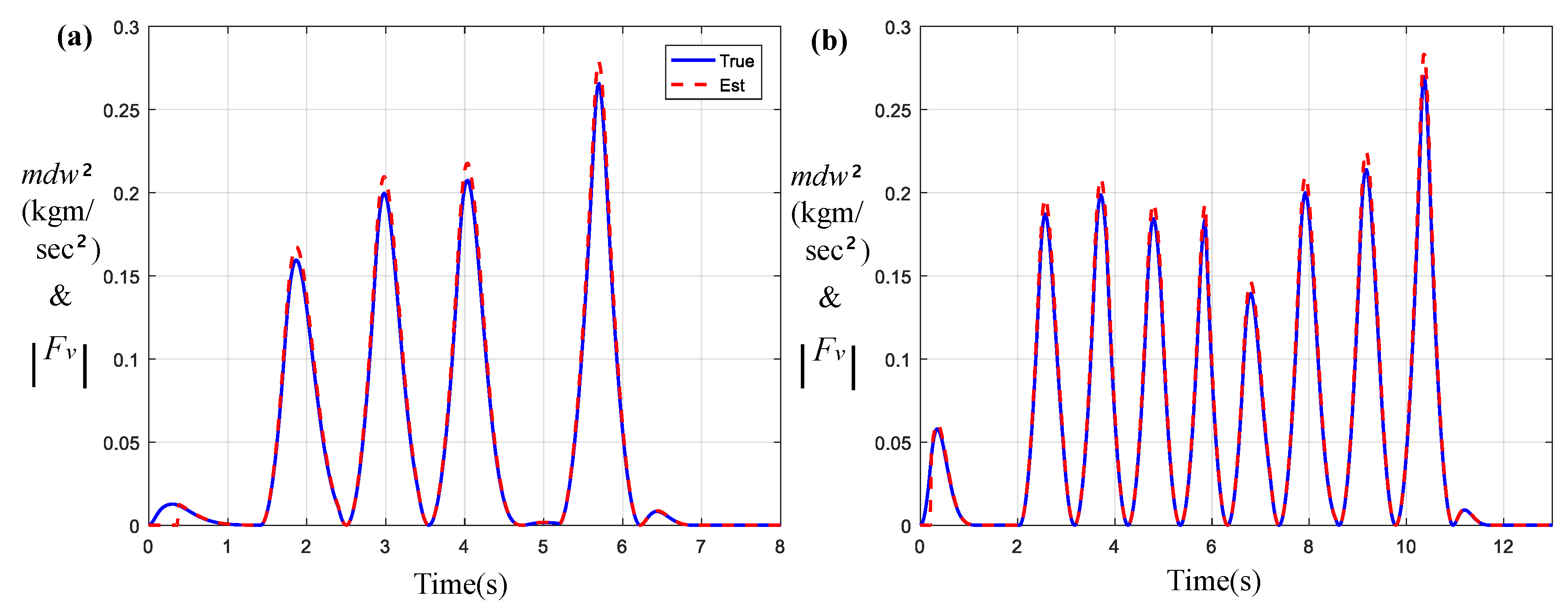
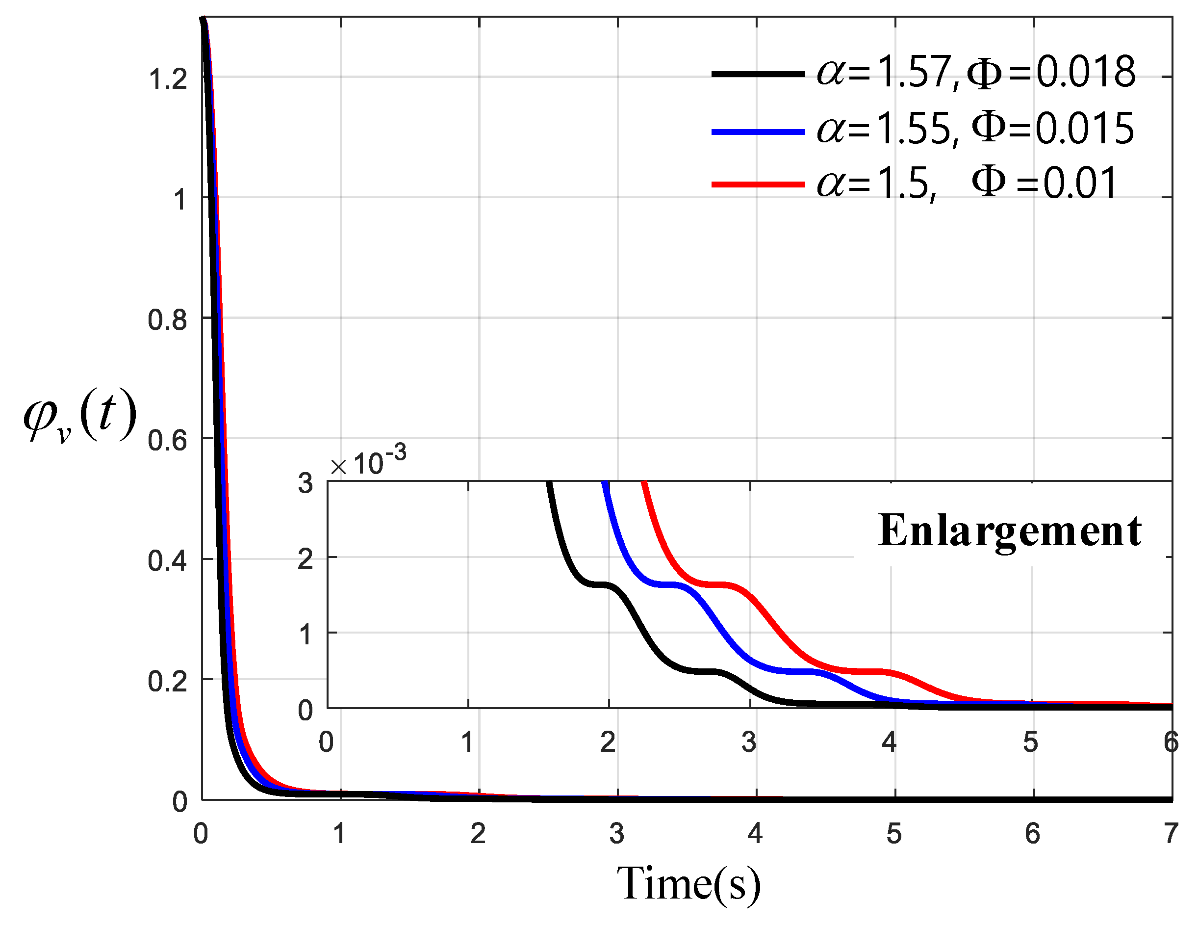
Figure 5 presents the estimation results of model uncertainty for Figure 3 and Figure 4. Here, $\gamma$ and $\rho$ are selected as 0.13 and 0.01 for d = 0.1. Due to the action of model uncertainty compensation term,$F_v$ it was found that the estimates |$F_v$| were well synchronized with the true values, resulting in cancelling the Coriolis effect of the WMR. In Figure 6, the (x,y)-navigation potential energies for three different tuning parameters have been presented. As the main parameters F and a of robust control increase, the convergence rate of potential energy became superior. For α = 1.57 and Φ = 0.018, the WMR touched down the zero level of potential energy within almost 3.7 s. This implies that those tuning parameters are very effective at manipulating the convergence rate resulting in possibly shortening the entire navigation time of the WMR. 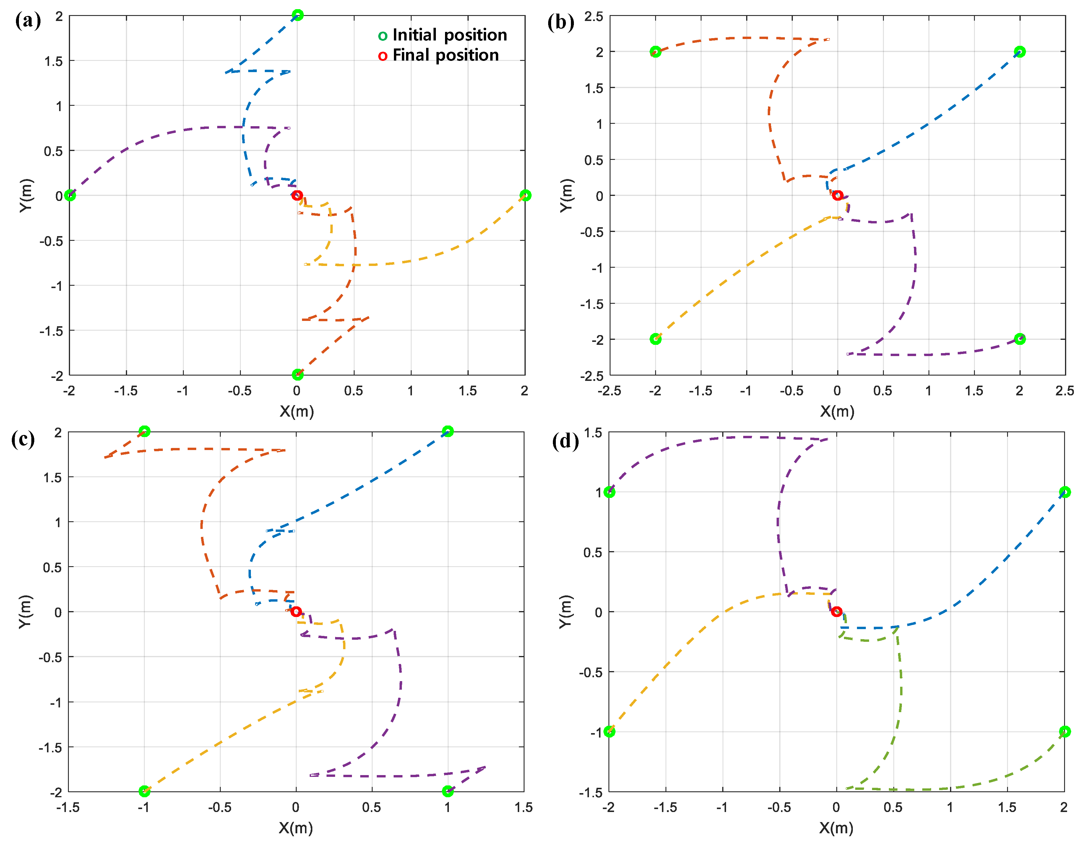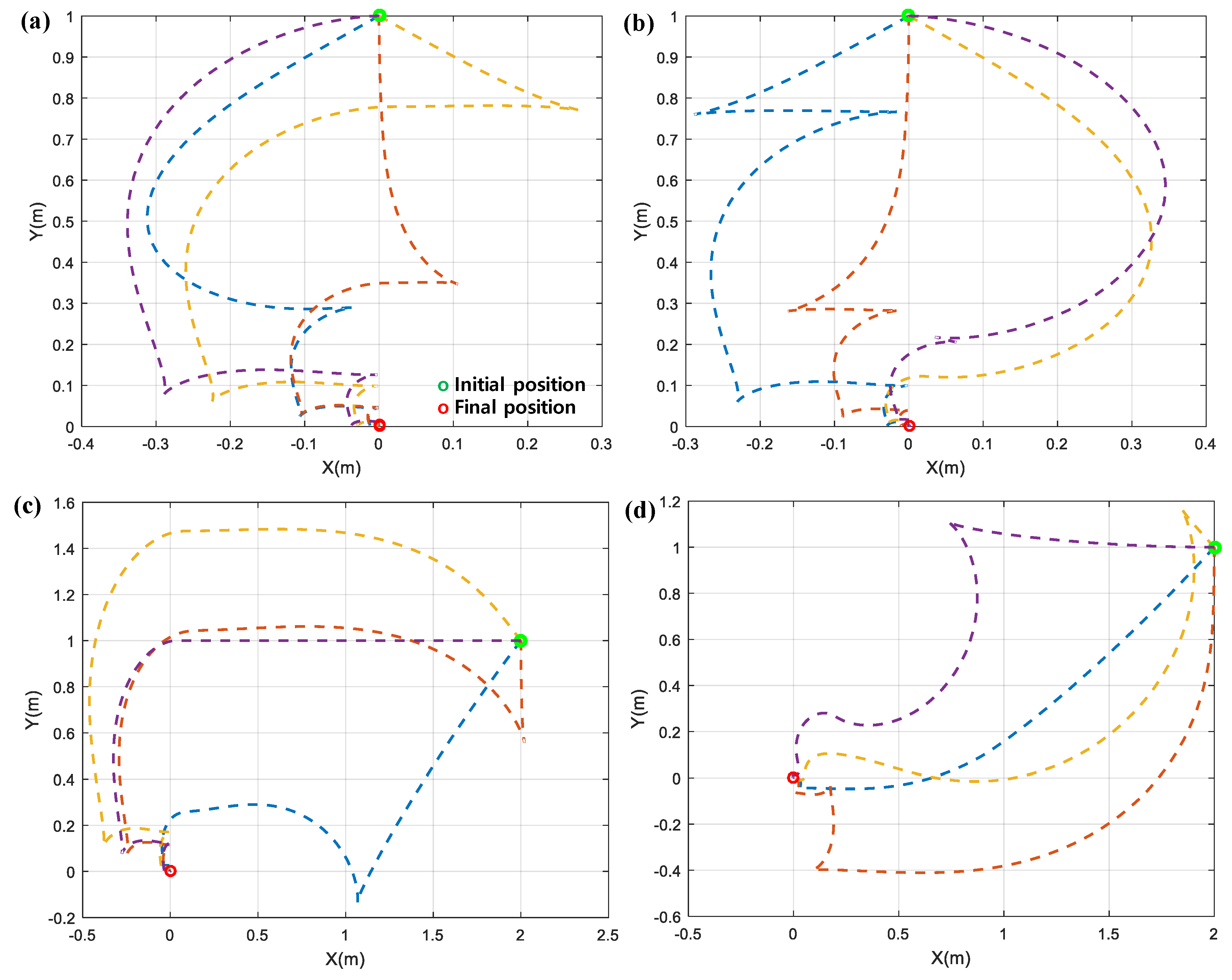As shown in Figure 7 and Figure 8, to explore the effectiveness of proposed control law in depth, various initial conditions were provided to the WMR. Specifically, Figure 7 includes the performance of WMR navigation for 16 different initial positions along with 45° orientation angle while Figure 8 includes the performance of the global convergences based on two different initial positions and eight different initial orientations. It is clearly seen from all simulation results that the WMR successfully passed through the forbidden sets (i.e., local minima) and pushed itself to the desired set of posture.

5. Conclusions

This paper presents a passivity-based switching control for the posture stabilization of a wheeled mobile robot with model uncertainty. The proposed technique ensures a finite control time between switches and guarantees the robustness for the model uncertainty which, in practice, cannot be negligible. The proposed control lawis totally designed based on the second order Largrangian dynamics (vs. first order kinematics based approach) without any complicated transformation and other accessories; thus it is compact and convenient to be implemented.

This paper also presents the fundamental Lyapunov-based robust control design and the study of the forbidden set (unwanted local minima) with a certain potential energy so that we could develop the idea of a switching law to avoid the set and accelerate the rate of global convergence. However, the convergence rate became slower as the robot approached the desired set, which is a common issue for the posture stabilization. Thus, the proposed technique intentionally chose the way that the WMR did not need to hesitate until the forward velocity became meaningless and it switched to another control law before losing its own navigation potential energy completely (i.e., switching at $\left|v\right|=\Phi \ne 0$). With this approach, it was unnecessary to set a greater perturbation angle of the second control law (as shown in Figure 3b and Figure 4b) as the WMR approached $E_d$. In other words, compared to the existing studies where the perturbation angle is required to be increased to obtain a certain level of forward velocity which enforces the strict decrease of the navigation potential energy, with the proposed technique the perturbation energy storing process is not as time-consuming. This possibly leads to a reducing in the total time for the navigation of WMR. It is hoped that this study could be another possible solution for the posture stabilization of second order wheel based non-holonomic dynamic systems with model unceratinity.

References

1. Peshkin, M.; Colgate, J.E. Cobots. Ind. Robot 1999, 26, 341. [Google Scholar] [CrossRef]
2. Weisbin, C.R.; Lavery, D. Nasa rover and telerobotics technology program. IEEE Robot. Autom. Mag. 1994, 1, 14–21. [Google Scholar] [CrossRef]
3. Levine, S.P.; Bell, D.A.; Jaros, L.A.; Simpson, R.C.; Koren, Y.; Borenstein, J. The navchair assistive wheelchair navigation system. IEEE Trans. Rehabil. Eng. 1999, 7, 443–451. [Google Scholar] [CrossRef] [PubMed]
4. Cortes, J.; Martinez, S.; Karatas, T.; Bullo, F. Coverage control for mobile sensing networks. IEEE Trans. Robot. Autom. 2004, 20, 243–255. [Google Scholar] [CrossRef]
5. Murray, R.M.; Li, Z.; Sastry, S.S. A Mathematical Introduction to Robotic Manipulation; CRC: Boca Ranton, FL, USA, 1993. [Google Scholar]
6. Colgate, J.E.; Schenkel, G. Passivity of a class of sampled-data systems: Application to haptic interfaces. J. Robot. Syst. 1997, 14, 37–47. [Google Scholar] [CrossRef]
7. Lee, D.J.; Spong, M.W. Passive bilateral teleoperation with constant time delay. IEEE Trans. Robot. 2006, 22, 269–281. [Google Scholar] [CrossRef]
8. Spong, M.W.; Holm, J.K.; Lee, D.J. Passivity-Based Control of Bipedal Locomotion. IEEE Robot. Autom. Mag. 2007, 14, 30–40. [Google Scholar] [CrossRef]
9. Arcak, M. Passivity as a design tool for group coordination. In Proceedings of the American Control Conference, Piscataway Township, NJ, USA, 13 August 2007. [Google Scholar]
10. Lee, D.J.; Li, P.Y. Passive decomposition approach to formation and maneuver control of multiple rigid bodies. ASME J. Dyn. Syst. Meas. Control 2007, 129, 662–677. [Google Scholar] [CrossRef]
11. De Wit, C.C.; SØrdalen, O.J. Exponential stabilization of mobile robots with nonholonomic constraints. IEEE Trans. Autom. Control 1992, 13, 1791–1797. [Google Scholar] [CrossRef]
12. Samson, C. Time-varying feedback stabilization of car-like wheeled mobile robots. Int. J. Robot. Res. 1993, 12, 55–64. [Google Scholar] [CrossRef]
13. Fierro, R.; Lewis, F.L. Control of a nonholonomic mobile robot: Back stepping kinematics into dynamics. J. Robot. Syst. 1997, 14, 149–163. [Google Scholar] [CrossRef]
14. Kolmanovsky, I.; Reyhanoglu, M.; McClamroch, N.H. Switched mode feedback control laws for nonholonomic systemsin extended power form. Syst. Control Lett. 1996, 27, 29–36. [Google Scholar] [CrossRef]
15. Hespanha, J.P.; Morse, A.S. Stabilization of nonholonomic integrators via logic-based switching. Automatica 1999, 35, 385–393. [Google Scholar] [CrossRef]
16. Hespanha, J.P.; Liberzon, D.; Morse, A.S. Logic-based switching control of a nonholonomic system with parametricmodeling uncertainty. Syst. Control Lett. 1999, 38, 167–177. [Google Scholar] [CrossRef]
17. Astolfi, A. Exponential stabilization of a wheeled mobile robots via discontinuous control. ASME J. Dynamic Syst. Meas. Control 1999, 121, 121–126. [Google Scholar] [CrossRef]
18. Bandyopadhyay, M.T.B.; Vachhani, L. Posture Stabilization of Unicycle Mobile Robot using Finite Time Control Techniques. IFAC-PapersOnLine 2016, 49, 379–384. [Google Scholar]
19. Lee, D.J. Passivity-based switching control for stabilization of wheeled mobile robots. In Proceedings of the Conference: Robotics: Science and Systems III, Georgia Institute of Technology, Atlanta, GA, USA, 27–30 June 2007. [Google Scholar]
20. Fujimoto, K.; Sugie, T. Stabilization of hamiltonian systems with nonholonomic constraints based on time-varying generalized canonical transformation. Syst. Control Lett. 2001, 44, 309–319. [Google Scholar] [CrossRef]
21. Hoang, T.T.; Duong, P.M.; Van, N.T.T.; Vinh, T.Q. Stabilization control of the differential mobile robot using Lyapunov function and extended Kalman filter. J. Sci. Technol. 2012, 50, 441–452. [Google Scholar]
22. Bessas, A.; Benalia, A.; Boudjema, F. Integral sliding mode control for trajectory tracking of wheeled mobile robot in presence of uncertainties. J. Control Sci. Eng. 2016, 2016, 7915375. [Google Scholar] [CrossRef]
23. Zaare, S.; Soltanpour, M.R.; Moattari, M. Voltage based sliding mode control of flexible joint robot manipulators in presence of uncertainties. Robot. Auton. Syst. 2019, 118, 204–219. [Google Scholar] [CrossRef]
24. Ibeas, A.; de la Sen, M. Robust sliding control of robotic manipulators based on a heuristic modification of the sliding gain. J. Intell. Robot. Syst. 2007, 48, 485–511. [Google Scholar] [CrossRef]
25. Rimon, E.; Koditschek, D.E. Exact robot navigation using artificial potential functions. IEEE Trans. Robot. Autom. 1992, 8, 501–518. [Google Scholar] [CrossRef]
26. Slotine, E.; Li, W. Applied Nonlinear Control; Prentice-Hall: Englewood Cliffs, NJ, USA, 1991. [Google Scholar]
27. KHALIL, H.K. Nonlinear Systems, 2nd ed.; Prentice-Hall: Upper Saddle River, NJ, USA, 1995. [Google Scholar]
Figure 1. A robot with the center of the mass at ( x c , y c ) and the geometric center at ( x o , y o ) with respect to the reference frame (o,x,y).
Applsci 09 05233 g001
Figure 2. (a) Transient scenario of forward velocity v(t) and (b) perturbation angle θ σ > 0 and θ ( t ) .
Applsci 09 05233 g002
Figure 3. Performance of robust switching control for initial condition (2,1) with 45°. (a) Trajectory of WMR on (x,y)-plane; (b) orientation of WMR θ(t); (c) (x,y) navigation potential energy; and (d) forward velocity of WMR v(t) (1st SW (Switching) in (a) indicates the position where the first switching occurs).
Applsci 09 05233 g003
Figure 4. Performance of robust switching control for initial condition (−1,0) with 45°. (a) Trajectory of WMR on (x,y)-plane; (b) orientation of WMR θ(t); (c) (x,y) navigation potential energy; and (d) forward velocity of WMR v(t) (first SW in (a) indicates the position where the first switching occurs).
Applsci 09 05233 g004
Figure 5. Model uncertainty estimation. (a) Case for Figure 3 and (b) case for Figure 4.
Applsci 09 05233 g005
Figure 6. Performance of switching control based on the tuning parameters (initial condition (2,1) with 45°).
Applsci 09 05233 g006
Figure 7. Trajectories of WMR for different initial positions. (a) Initial positions (2,0), (0,2), (−2,0), and (0,−2); (b) initial positions (2,2),(−2,2),(−2,−2), and (2,−2); (c) initial positions (1,2),(−1,2),(−1,−2); and (1,−2), and (d) initial positions (2,1),(−2,1),(−2,−1), and (2,−1).
Applsci 09 05233 g007
Figure 8. Trajectories of WMR for different initial orientations. (a) and (c) Initial orientations −135, −90, −45, and 0°; (b) and (d) initial orientations 45, 90, 135, and 180°.
Applsci 09 05233 g008