Article

Correlation Analysis between UBD and LST in Hefei, China, Using Luojia1-01 Night-Time Light Imagery

1
School of Geographic Sciences, Nantong University, Nantong 226007, China
2
School of Economics and Management, Nantong University, Nantong 226019, China
3
Department of Land Surveying and Geo-Informatics, The Hong Kong Polytechnic University, Hong Kong, China
4
Key Laboratory of Virtual Geographical Environment, MOE, Nanjing Normal University, Nanjing 210046, China
*
Author to whom correspondence should be addressed.
Appl. Sci. 2019, 9(23), 5224; https://doi.org/10.3390/app9235224
Submission received: 6 November 2019 / Revised: 27 November 2019 / Accepted: 28 November 2019 / Published: 1 December 2019
(This article belongs to the Section Earth Sciences)

Abstract

:
The urban heat island (UHI) is one of the essential phenomena of the modern urban climate. In recent years, urbanization in China has gradually accelerated, and the heat island effect has also intensified as the urban impervious surface area and the number of buildings is increasing. Urban building density (UBD) is one of the main factors affecting UHI, but there is little discussion on the relationship between the two. This paper takes Hefei as the research area, combines UBD data estimated by Luojia1-01 night-time light (NTL) imagery as the research object with land surface temperature (LST) data obtained from Landsat8 images, and carries out spatial correlation analysis on 0.5 × 0.5 km to 2 × 2 km resolution for them, so as to explore the relationship between UBD and UHI. The results show the following: (1) Luojia1-01 data have a good ability to estimate UBD and have fewer errors when compared with the actual UBD data; (2) At the four spatial scales, UBD and LST present a significant positive correlation that increases with the enlargement of the spatial scale; and (3) Moreover, the fitting effect of the Geographically Weighted Regression (GWR) model is better than that of the ordinary least squares (OLS) regression model.

Graphical Abstract

1. Introduction

With rapid development and the intensification of urbanization, the scale of cities has expanded rapidly and urban buildings tend to be denser, which brings more pressure on the population, transportation, and industrial production, and causes severe damage to the ecological environment of the entire city. Urban Heat Islands (UHIs) are attracting more and more attention, especially in summer, as scorching hot temperatures have severely affected people’s lives and work [1,2,3]. To date, researchers all over the world have carried out much research on UHIs. Among this research, quantitative analysis of the relationship between urban Land Surface Temperature (LST) and the underlying surface has become a research hotspot [4,5,6,7]. Scholars believe that urbanization changes the atmospheric dynamics and heat transfer characteristics of the underlying surface as a large number of natural landscapes are gradually replaced by urban impervious surfaces such as buildings and pavements. This makes the urban landscape fragmented and complicated, which changes the urban ground energy balance [8]. Under the same environmental conditions, impervious surfaces absorb and capture solar radiation faster than green space or other natural underlying surfaces. At the same time, the artificial structure absorbing heat faster and the specific heat capacity being smaller gives rise to limited heat release. In this way, the average LST in the area gradually increases with the spatial distribution of the UHI area to become more continuous and concentrated, forming a high-temperature area centered on artificial buildings in the city [1,9,10]. However, our comprehensive literature research found that past studies focused on the analysis of seasonal, daily, and annual variations of the UHI, which revealed the temporal and spatial variation of the UHI, the distribution characteristics of the horizontal and vertical directions, etc., while there has been less quantitative analysis of the single factors of UHIs, especially discussion of the ubiquitous relationship between impervious surfaces and UHI in the city.
As an integral part of the urban impervious surface percentage, the urban building density (UBD) (percentage of built area) can directly reflect the degree of intensification and land-use efficiency in cities to some extent [11]. It is also an essential comprehensive social indicator that can function as an urban planning layout measure [12,13], resource utilization efficiency measure [14,15], and assessment of the urban ecological environment and livability [16,17,18,19]. Some researchers have pointed out that UBD is a crucial indicator to reduce the UHI effect [20] and proved a positive correlation between UBD and LST or UHI [21,22,23]. Additionally, researchers have tried to use a variety of urban design factors to study the relationships of UHIs, including UBD information. For example, Yang studied the summer heat island intensity of three high-rise residential districts in Shanghai, based on the three indices of building layout, density, and greening [1]. Hu used nine urban design factors to construct the Sky View Factor (SVF), studied high-density urban areas with high UHI and low SVF as the research object, and tested the possibility of UHI by optimizing the urban-form SVF [24].
Remote sensing technology, as an accurate and timely means to obtain macroscopic information on the Earth’s surface, has been widely used in many fields [25]. Thermal infrared remote sensing technology is a common means of monitoring LST [26,27]. Using remote sensing images to extract UBD information is also a fast and effective method to make up for the shortcomings of traditional manual mapping methods. Existing studies on UBD tend to use high-resolution remote sensing satellites for research because they are more accurate [11,28,29], but their shortcomings are also obvious, such as complex building analysis, the cumbersome automated extraction process, and a large number of computations.
NTL remote sensing is widely used in macroeconomic and social parameter estimation [30,31,32], urban monitoring [33,34,35,36], great event change [37,38], energy consumption [39,40], ecological environment assessment [41,42], and other fields. Due to the low spatial resolution of NTL images, previous studies focused on macroscopic dimensions, such as national or urban scales. However, urban buildings with small-scale features are the basic unit of human activities. More sophisticated data and advanced means are needed in terms of reasonable arrangements and scientific planning for the limited land in a city, reduction of UHIs, and better ecological effects. Therefore, medium- and high-resolution NTL sensors have become an urgent requirement for urban research. On 2 June 2018, the Luojia1-01 scientific test satellite successfully launched; it carries a large-field-of-view, high-sensitivity NTL remote sensing camera with 130 m resolution and 260 km width NTL imaging capability. Compared with commonly used NTL data such as that from the Defense Meteorological Satellite Program’s Operational Linescan System (DMSP-OLS) and Suomi National Polar-Orbiting Partnership’s Visible Infrared Imaging Radiometer Suite (NPP-VIIRS), Luojia1-01 NTL imagery is a remarkable improvement in terms of spatial resolution, image saturation, and blooming effects [43]. Conducted to provide frontier data, the current research based on Luojia1-01 NTL imagery is expanding. Luojia1-01 NTL imagery has been applied to the drawing of urban range [44], extraction of impervious surfaces [45], and urban economic estimation [46,47]. However, it is not clear whether it is feasible to estimate UBD information using Luoji1-01 NTL imagery, and there is little quantitative analysis of the single factors giving rise to UHI, especially discussion of the spatial relationship between UBD and LST. As we seek to address these problems, the purpose of this paper is to (1) test the feasibility of Luojia1-01 NTL imagery for UBD estimation; (2) combine the UBD estimation with LST data obtained from the Landsat8 data inversion; and (3) use the Geographically Weighted Regression (GWR) model and the spatial analysis method of the ordinary least squares (OLS) regression model to study the spatial relationship between UBD and LST in order to provide a scientific basis for the planning of urban construction layout and urban thermal environmental management.

2. Study Area and Data

2.1. Study Area

Hefei, the capital of Anhui Province, is situated in the center of Anhui Province, eastern China (31.51 N, 117.17 E). It is also included as a key city in the national strategy for the development of central China. Hefei covers a total area of 11,445 square kilometers and has municipal districts (Yaohai, Luyang, Shushan, and Baohe), one county-level city (Chaohu city), and four counties (Changfeng, Feidong, Feixi, and Lujiang). As of 2018, the city’s permanent population was 8.087 million, and the main urban population was 3.938 million. Figure 1 is the area change data of each land type in Hefei in 15 years obtained from the Geographical Information Monitoring Cloud Platform (http://www.dsac.cn/DataProduct/Detail/20091601998301300). During the past 15 years, the vegetation coverage of Hefei City has been decreasing year by year, and the urban area has been expanding. Urbanization has brought many environmental problems in the city, and the UHI effect is one of them. This prompts us to ask how to maintain a balance between urban development and livability. Based on this background, this paper takes Hefei city as an example to analyze the four municipal districts, Yaohai, Xiangyang, Lushan, and Baohe, as shown in Figure 2.

2.2. Experimental Data

2.2.1. Luojia1-01

Luojia1-01, successfully launched at JSLC (Jaquan Satellite Launch Centre) on 2 June 2018, is a scientific experimental microsatellite jointly developed by Wuhan University and CGSTL (Chang Guang Satellite Technology Co., Ltd., Changchun, China). It is not only the first professional night-time light remote sensing satellite in the world but also the first low-orbit satellite with Earth observation and satellite navigation enhancement functions. It is capable of forming images with 130 m resolution and 250 km wide fields. Moreover, the Luojia1-01 satellite is ideally able to take global night-light images and provide data within 15 days, which provides a basis for measuring the global gross domestic product (GDP), the carbon emission index, and the urban housing vacancy index [48]. All of these data can be downloaded free from the Hubei Data and Application Network of the High-Resolution Earth Observation System (http://59.175.109.173:8888/app/login.html).
For this paper, we selected Luojia1-01 NTL imagery from 15 July 2018, with better image quality, i.e., cloudless data. Then, we converted the digital number value (DN) to the spectral radiance by radiation correction [46]. The following radiance conversion formula was as follows:
L = D N 3 2 10 10
where L is the radiance value after absolute radiation correction, for which the unit is W / ( m 2 · μ m · sr ) . The D N value is the gray value of the image.

2.2.2. Landsat8

Landsat8 thermal infrared sensor (TIRS) data were utilized to analyze the LST. They were issued by the United States Geological Survey (USGS) Global Visualization Viewer (GloVis, https://glovis.usgs.gov). To be consistent with the time of the Luojia1-01 data, we analyzed all images (with less than 10% cloud cover) available for a three-months time period from 1 June to 30 August 2018. After this analysis, we chose the cloud-free image from 30 July, with path 121 and row 038. As we were looking to reduce the influence of terrain, illumination, and atmosphere on the spectral information, we performed radiation calibration and atmospheric correction on the image. The Radiation Correctiong module sub-tool, Radiometric Calibration in ENVI software, is used to perform the radiometric calibration on the TM image in the study area, and the FLAASH module is used for atmospheric correction.

2.2.3. Other Auxiliary Data

ZY3-02 sensor-corrected products were acquired on 18 July 2018, provided by the China Centre for Resources Satellite Data and Application (CRESDA, http://www.cresda.com/CN/), since the planimetric and vertical accuracies of the ZY3-02 sensor-corrected products are better than 2.5 m and 2 m, respectively [49]. We used the forward/backward stereo images to assist with Luojia 1-01 image geometric correction and extract the building digitization.
In addition, the Hefei city Regional Map of the study area can be obtained from the Tianditu net (http://map.tianditu.gov.cn). In order to maintain consistency between different data sources, all remote sensing data were first converted into a WGS_1984_Albers projected coordinate system. The study area, as captured by the different data sources, is shown in Figure 3.

3. Methodology

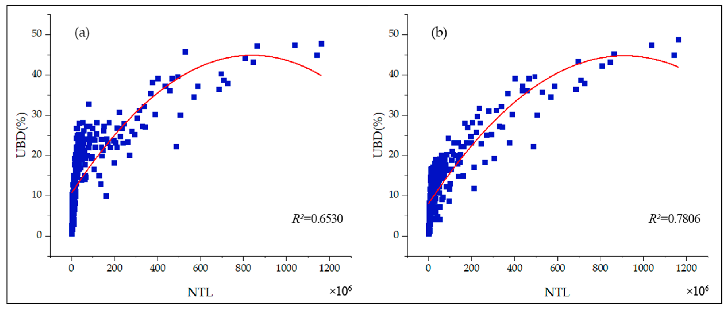
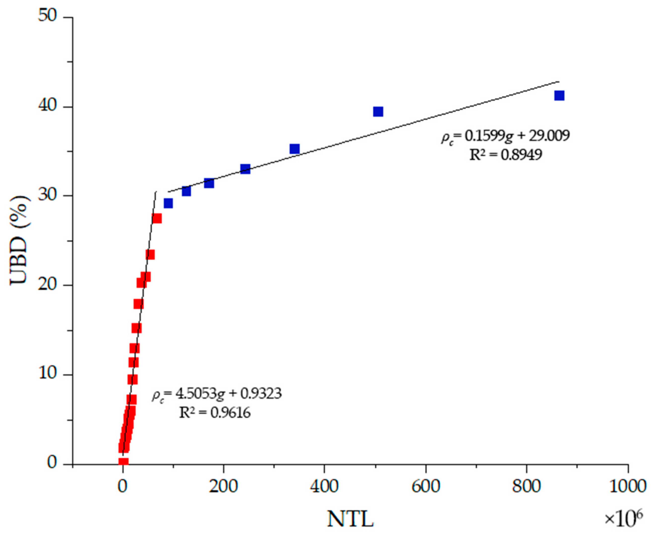
3.1. UBD Estimation Model and Verification

To achieve a small scale for research purposes and reduce the error in the research results, the estimation of the UBD is generally calculated in units of fixed-size grid cells. Considering the spatial resolution of the Luojia1-01, each sample area was divided into 0.5 × 0.5 km by testing the side length of the cell. Then, the radiance value of the study area was divided into 32 classes of NTL intensity by the natural breakpoint grading method, and 10 sample areas were set for each class of NTL intensity. According to the principle of equilibrium distribution, in this article we tried to avoid the boundary of the study area when selecting samples; finally, we set up 320 samples areas for modeling and randomly selected another 20 areas as test samples, as shown in Figure 4a.
The area of a building’s roof can usually be used instead of the area of the building for UBD calculations. Combined with the ZY3-02 orthophoto with a high resolution of 2.5 m, the building area can be obtained by digitizing all the buildings in each sampling area in turn. Figure 4b,c shows an example of building digitization. Through calculating the UBD of the 320 sample areas, we obtained a calculation result which can be regarded as the actual UBD of the sample area. The calculation formula is shown as follows:
ρ a i = S a i / S
where ρ a i ˙ is the UBD of the the i ˙ -th sample area; S a i is the building area of the i -th sample area; and S is the area of the sample area, which is 0.5 × 0.5 km.
Among the various land use types, high-brightness lighting is widely used in the transportation field, while residential areas have low illumination; this can explain why the lighting along the roads is one factor in UBD estimation [43]. In recent years, researchers have used many methods to extract road information from high-resolution remote sensing images. In this paper, referring to the method in references [50,51,52], the road area information of the 320 modeling samples was extracted from ZY3-02 high-resolution images and overlapped with the Luojia1-01 NTL imagery to reduce the interference of road light sources in the UBD estimation model. Figure 5 is a schematic diagram of the entire process.
Step 1: Perform grayscale processing on the original image from ZY3-02. The Mean-Shift algorithm was used to achieve the initial segmentation of the road. The setting of the dual-threshold can better distinguish the features of different gray levels and eliminate the interference of small-area shadows such as vegetation and vehicles. Finally, the binarized image containing road information is segmented.
After binarization, dual-threshold segmentation can well overcome the differences caused by the different gray levels of various road materials since the spectral differences between shadows, green spaces, and roads are then apparent. In the process of Mean-Shift algorithm segmentation, combined with small-area segmentation and the dual-threshold segmentation method, most interfering factors can be eliminated.
Step 2: For the binarized image, there is mainly interference from other artificial objects such as buildings, and the buildings are usually a combination of regular rectangular shapes, but the roads are strip-shaped. The shape feature processing should be conducted to the image because roads have a certain width. By calculating the area of the segmented region and setting a certain threshold, it is possible to effectively remove small patches that may exist after the binarization process. Rectangularity is a measure of the target rectangle, which is defined as the ratio of the area of the target graph to the smallest rectangle area surrounding the graph. The formula of rectangularity is as follows:
S = S o / S m ,
where S o is the area of the target graph; S m is the area of the smallest rectangle surrounding the graph. S can indicate how close the target object is to the rectangle. The range of rectangularity is (0, 1).
The aspect ratio can reflect the slenderness of the object, and it can be used to extract areas with significant length features. Aspect ratio is expressed as:
R = L m / W ,
where L m the length of the minimum circumscribed rectangle; W is the width of the smallest circumscribed rectangle.
In this paper, the area, the aspect ratio, and the rectangularity were respectively set to 20, 2.5, and 0.36. Extensive use of these features can effectively remove non-road targets that are isolated from the road. Furthermore, through further processing by morphological filtering, the road edge is refined and smoothed to obtain the final road information [53].
Step 3: As the brightness value around the road is higher than the actual values in the Luojia1-01 images, the extracted road information was used to cover the Luojia1-01 NTL imagery, and K-means clustering was used for Luojia1-01. The principle is to cluster the brightness values around the road in order to take the average value and fill the brightness value of the road.
From the comparison shown in Figure 6, we can see that eliminating the interference of road light sources improved the accuracy: the correlation between the sample area NTL and the actual UBD was raised from 0.6530 to 0.7806.
After stripping the road area of the sample area, the UBD values of samples of the 32 types of NTL intensity were averaged, and the calculation formula was as follows:
ρ c * = i = 1 N ( S a i S b i ) ( S × N ) = i = 1 N ( ρ a i ρ b i ) N
where ρ c * is the average UBD of the   c -type NTL intensity sample area;   N   is the number of samples; ρ a i   is the UBD of the   i th sample in the   c -type NTL intensity sample area; ρ b i   is the density of the road in the i th sample area of the c -type NTL intensity sample area; S is the area of the sample area; S a i is the construction area of the   i th sample area of the   c -type NTL intensity sample area; and S b i   is the road area of the   i th sample area of the   c -type NTL intensity sample area.
A segmented linear regression was used to fit the relationship between the average building density and the light intensity in the 32 sample areas, and the average UBD estimation model under different NTL intensities was obtained by:
ρ c = { 4.5053 g + 0.9323 , 0 < g 14.319 0.1599 g + 29.009 , g > 14.319
where   g   is the brightness of Luojia1-01 NTL and   ρ c   is the average UBD of the NTL intensity classification sample area.
Figure 7 is a schematic diagram of the segmented linear regression with a coefficient R 2   of 0.9616 and 0.8949. The segmented linear regression model was used to calculate the statistics of the fitting results of the average building density of the 32 types of NTL intensity samples, as shown in Figure 8.
The spatial analysis tool in ArcGIS10.3 software was used to spatially interpolate the UBD values of the 320 sampling points to obtain the overall distribution map of UBD in the main urban area of Hefei City (Figure 9); Table 1 gives the detailed UBD distribution data. The formula for the inverse distance weighted (IDW) method is as follows:
ρ c = i = i N ρ c i / d c i 2 i = i N 1 / d c i 2
where   ρ c   is the value of the UBD estimate for the   c -type NTL intensity sample area;   N   is the number of samples;   ρ c i   is the average value of the UBD at the center point of the   i th sample in the   c -type NTL intensity sample area; and   d c i   is the distance between the center point of the   i th sample and the   c -point.
The actual UBD values of 20 test samples were obtained from ZY3-02 high-resolution images, and the final estimation results were tested. As shown in Table 2, the absolute UBD error of 11 in 20 test plots was less than 5%, and there are only 2 plots with an absolute error higher than 10%. From the average result, the absolute difference between the UBD of the sample area and the estimated UBD was 3.58%, which proves that the estimation result is highly reliable. For a single data, the estimated UBD for the high-density region is generally higher than the actual UBD because the high-density region has more interfering light sources and the blooming effect results in a larger estimated building area than the actual one. From the absolute error, the absolute error for the low-value region of the average luminance value is smaller than that for the high-value region. The reason for this is that the NTL intensity of the low-value zone is smaller, and a more realistic light index can be monitored at night.

3.2. LST Retrieval from Landsat8

Conventional methods based on Landsat8 TIRS surface temperature inversion include the radiative transfer equation (RTE) method, single-channel method, and split-window algorithm. Some scholars have carried out quantitative comparison analysis on the inversion precision of the different algorithms. The results showed that the radiation transfer equation method has the highest precision [27]. The basic principle of the radiation transfer equation method can be illustrated as follows: firstly, the influence of the atmosphere on the surface heat radiation is estimated, then these effects are subtracted from the total heat radiation amount observed by the satellite sensor, and the surface heat radiation intensity is finally obtained and converted into the LST.
The Landsat8 TIRS has two thermal infrared bands (bands 10, 11), but the calibration parameters for the TIRS band 11 are not stable; thus, we selected the Landsat8 TIRS band 10 on which to use the RTE method to invert the surface temperature. The calculation formula is as follows.
The thermal infrared radiation brightness value L λ   received by TIRS consists of three parts: the atmospheric transmissivity ( τ ), the atmospheric upward radiation ( L ), and the atmospheric downward radiation ( L ). We use the atmospheric correction parameter calculator website provided by NASA (https://atmcorr.gsfc.nasa.gov/) to get these values, where τ is 0.47, L is 4.93 W / ( m 2 · μ m · sr ) , and L is 7.18 W / ( m 2 · μ m · sr ) .
The RTE of the thermal infrared radiance L received by the TIRS is as follows:
L λ = L + [ ε B ( T s ) + ( 1 ε ) L ] τ
where   ε   is the land surface emissivity; T   is the real temperature of the surface; B ( T s )   is the radiance of the blackbody at temperature T   in the thermal infrared band; and τ   is the atmospheric transmittance in the thermal infrared band.
Remote sensing estimation of Vegetation Fractional Cover (VFC) refers to the vertical projected area of vegetation as a percentage of the total area of the study area. It reflects the degree of vegetation and the size of the photosynthesis area of the plant. At present, the more mature VFC estimation method is dimidiate pixel mode, which is estimated by the Normalized Difference Vegetation Index (NDVI). NDVI can be expressed as:
N D V I = N I R R N I R + R
V F C = ( N D V I N D V I S ) / ( N D V I V N D V I S )
where N I R is for near-infrared reflectivity; R is red band reflectivity; N D V I S is the N D V I value of bare land; and N D V I V is the N D V I value of vegetation.
On the scale of pixels, surface features are mainly divided into three types: natural surface, water body, and urban building. The natural surface is the main body in the composition of the ground, so the natural surface is the main body of temperature inversion. The formula for calculating the surface emissivity is as follows:
ε s = 0.9625 + 0.0614 V F C 0.0461 V F C 2
ε b = 0.9589 + 0.086 V F C 0.0671 V F C 2
where ε s is the surface emissivity of the natural surface; ε b is the surface emissivity of the built-up area.
B ( T s )   can be expressed as:
B ( T s ) = [ L λ L τ ( 1 ε ) L ] / τ ε
According to Plank’s law, T s   can be expressed as:
T s = K 2 ln ( K 1 B ( T s ) + 1 )
In TIRS Band 10, K 1   and K 2   are constant: K 1 = 774.89   W / ( m 2 · μ m · sr )   and   K 2 = 1321.08 K .
It is necessary to verify the accuracy of the inversion for the reason that all kinds of LST inversion methods errors exist. The MOD11A1 LST data of the same day is used as the reference value of Hefei LST. The fishnet is used for grid processing, figuring out the mean value of temperature in each grid and carrying on the correlation analysis. As shown in Table 3, the surface temperature obtained by the RTE method differs very little from the maximum and average values of the MOD11A1 data. At the same time, the correlation coefficient between the two is 0.94, which is very significant at a confidence level of 0.001. The results show that the LST retrieved by the RTE method meets the research needs.
Finally, we converted the LST raster data into vector data, and the accordance means—standard deviation method was employed to transform the LST into a thematic map of five thermal categories: low, sub-low, middle, sub-high, and high, as shown in Figure 10. The basis of this grading and the temperature ranges corresponding to the different temperature levels are shown in Table 4.

3.3. Geographically Weighted Regression

Geography objects, such as a change in the pattern, the distribution of time and space, and the mutual coupling relationship, are scale-dependent, which means that a specific relationship within the geographical aspect may only be expressed on a certain scale [54]. The study area was divided into four spatial scales of 0.5 × 0.5 km, 1 × 1 km, 1.5 × 1.5 km, and 2 × 2 km, and the average UBD and average LST in each grid were determined. The UBD data were logarithmically transformed to make the data population normally distributed. Then, the Pearson correlation coefficient between the UBD and LST was calculated, and a linear regression analysis using the bivariate regression model was used to explore the correlation between LST and UBD.
As shown in Figure 11, UBD and LST showed a significant positive correlation at each of the four grid scales, the degree of correlation increased in pace with the spatial scale, and the correlation coefficient reached a maximum at the scale of 2 km. This shows that the distribution of the UBD has a warming effect on the LST at the fine-scale of the city, and the contribution UBD makes to the LST at the grid-scale of 2 km was greater than that at the other three scales. Due to the small scale of analysis and more complex factors affecting the LST, more variables need to be considered, such as local airflow and the regional surface three-dimensional structure. Therefore, the impact of LST decreases with increasing spatial scale, and the correlation between UBD and LST is stronger. The bivariate regression model ( R 2 = km 22) established on the 2 km grid-scale, although having certain interpretation and prediction capabilities, is not enough to express the spatial relationship between UBD and LST.
We applied GWR and ordinary least squares (OLS) regression to further analyze the relationship between the UBD and LST. The traditional regression model is based on the use of OLS to estimate the parameters and is usually compared as a benchmark model with an improved model [55,56,57]. OLS can be expressed as:
Y k = β 0 + i = 1 k β i X i + ε k
where Y k denotes the global dependent variable; X i   is the   i th index of the independent variable;   β 0   represents the intercept value; i   is the number of indicators; β i is the slope coefficient; and ε denotes the random error term.
GWR is characterized by incorporating the spatial characteristics of data into the model to create conditions for analyzing the spatial characteristics of the regression relationship [10,47]. The GWR model is expressed as:
Y k = β 0 ( u i , v i ) + i = 1 k β i ( u i , v i ) X i + ε k
where ( u i , v i ) denotes the spatial coordinates of point   i ;   X i   is the   i th index of the independent variable; β 0 ( u i , v i ) is the intercept value; β i ( u i , v i ) represents the i th slope coefficient at point i ; and ε denotes the random error term.
The weight is usually calculated by using a Gaussian function when correcting GWR. The Gaussian function is expressed by the following formula:
W i j = e x p 1 2 ( d i j b ) 2
where d i j   denotes the Euclidean distance between location i and j ; and b   is the fixed bandwidth for location i .
Before establishing regression models and analyzing, it should be judged as to whether there is a spatial correlation in the variables. The index commonly used is Moran’s I. A scale of 2 km is suitable for studying the UBD—LST relationship in the main urban area of Hefei. The difference between the LST in different places depends mainly on the construction within 2 km of these places. Then, 2 km will also be a reasonable measure for calculating Moran’s I. As shown in Figure 12, with a 2 km scale, the Moran’s I value of the LST was 0.3948, the p -value was 0.0008, and the z score was 3.3532. This indicates that the LST in the study area is agglomerated and distributed, the spatial difference is vast, and there is spatial autocorrelation in the study area.

4. Results and Analysis

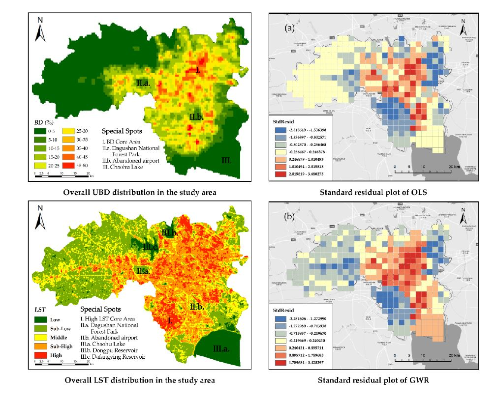
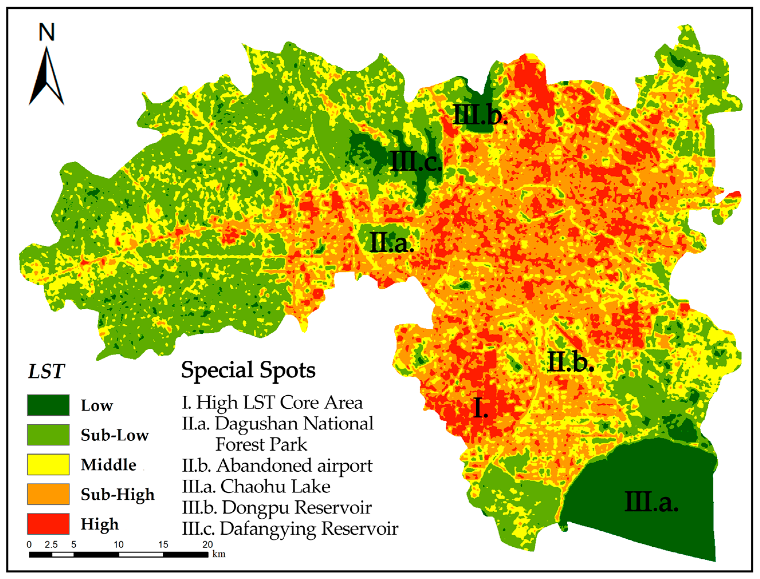
4.1. Spatial Distribution of UBD and LST

Taking the main urban area of Hefei City as the research area (including the urban waterbody), the UBD obtained from Luojia1-01 NTL imagery is consistent with the spatial pattern characteristics of the LST obtained from Landsat8 TIRS.
From the overall distribution results of the study area UBD (Table 1), we can state the following: The proportion of the low-density area is the largest, reaching 47.06%; and the low-density areas are mainly distributed in the outer suburbs with high vegetation coverage, few buildings, and small human development space. Besides this, the area ratio of the middle-density area is 24.60%, and the high-density area and sub-high-density area take up less than 10%. The UBD value of Binhu New Town is the highest, reaching 48.25%. This area is an emerging urban circle developed in Hefei City in recent years, and it has had a new agglomeration effect on the UBD.
Table 3 shows that the LST range of the study area is between 19.21 °C and 46.14 °C, with an average LST of 27.44 °C and a standard deviation of 4.72 °C. The spatial distribution of the LST is shown in Figure 10. The area of the sub-low temperature zone in the study area is the largest, accounting for 33.87%, and the sub-high temperature zone is also large (25.77%); the high-temperature zone and the low-temperature zone is the smallest. The area with LST larger than 26.97 °C is basically concentrated in the urban area, while the LST in the suburbs is mostly between 23.06 °C and 26.97 °C. The LST is quite different between the urban and suburban areas, and the UHI effect is significant.
The partial views of Figure 9 and Figure 10 show that there are three typical areas in the entire study area: the high-concentration areas for the LST and UBD are different in terms of geographic location. Figure 9 (I.) shows that the most concentrated areas of the high-density area are located at the intersection of four jurisdictions in Hefei City, with an average UBD greater than 25%. The area is an old town with numerous high-rise buildings, a dense population, low greening rate and fragmentation, and dense road networks. In Figure 10 (I.), the densest and most continuous location in the high-temperature zone is in the southern part of the study area. By comparing remote sensing images, it was found that in addition to industrial production and anthropogenic heat emissions, there are a large number of low-rise industrial buildings and hard pavements which absorb a large amount of heat and lead to an increase in temperature.
As shown in Figure 10 (II.a. and III.a.,b.,c.), the low-temperature area is mainly concentrated in urban water bodies and forest parks. The water body and vegetation effectively cut off the high-temperature area and increase the fragmentation degree of the urban LST, while playing an essential role in relieving the UHI effect and the local thermal environment. Besides this, the values of LST and UBD at II.b. are significantly lower than those in the surrounding area. The remote sensing image showed that the area is an abandoned airport in Hefei which has high vegetation coverage and low UBD.
The obtained UBD layer and the inversion LST layer were superimposed and analyzed. The results showed that the average temperature of the high-density area in the study area is 30.50 °C, and the average temperature of the sub-high-density zone is 27.35 °C. The average temperature of the middle-density zone is 26.31 °C, the average temperature of the sub-low-density zone is 23.32 °C, and the average temperature of the low-density zone is only 21.05 °C. Therefore, UBD has a warming effect on the thermal environment inside the city. Moreover, the LST increases with the UBD; especially at a specific scale, this warming effect is more obvious.
In general, (a) the overall trend of the UBD and LST is a decline from the core area of the city to the periphery; (b) the density of buildings and the spatial distribution of the LST are affected to some extent by the terrain; and (c) the two data distribution characteristics are the same, but there are differences in local areas.

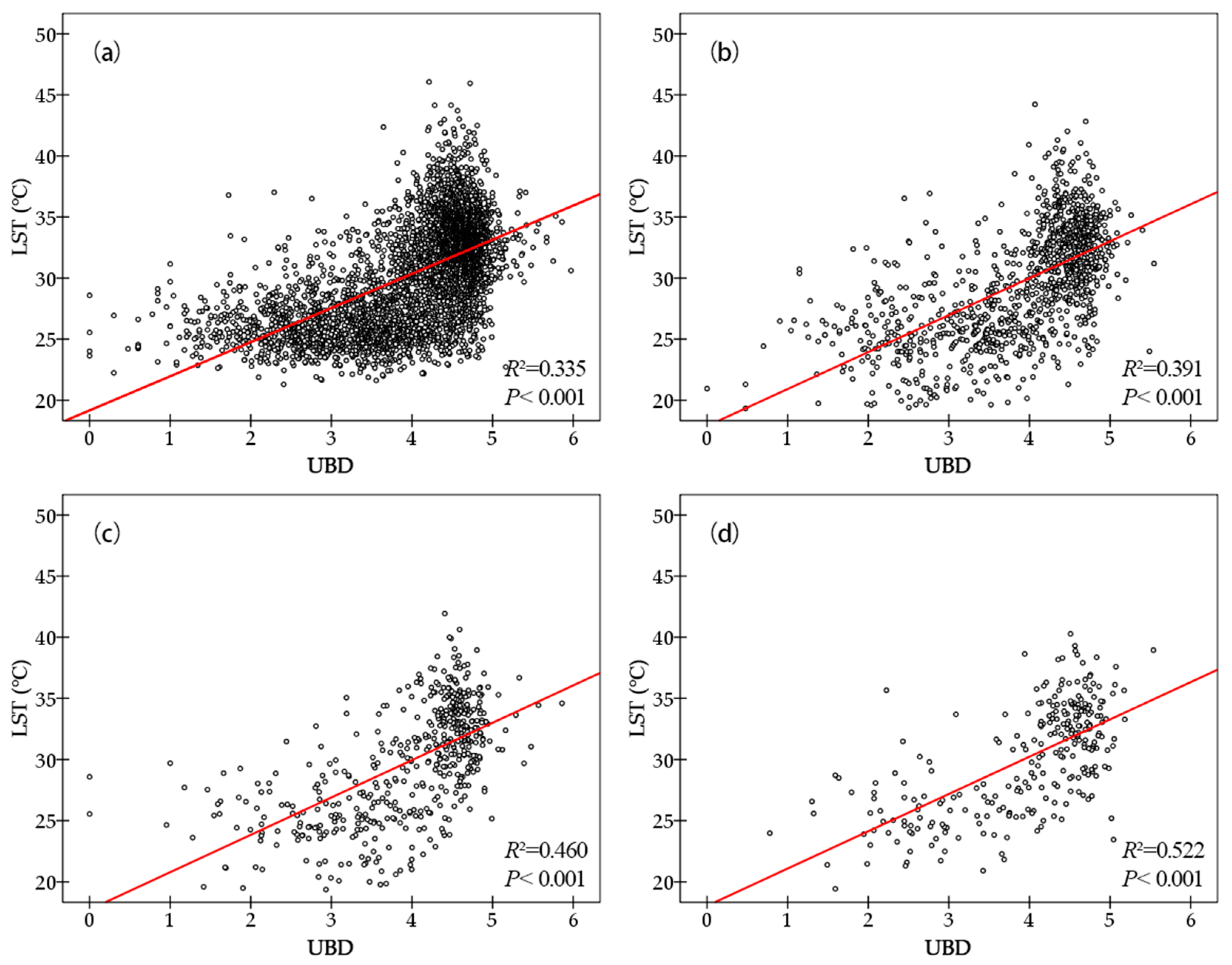
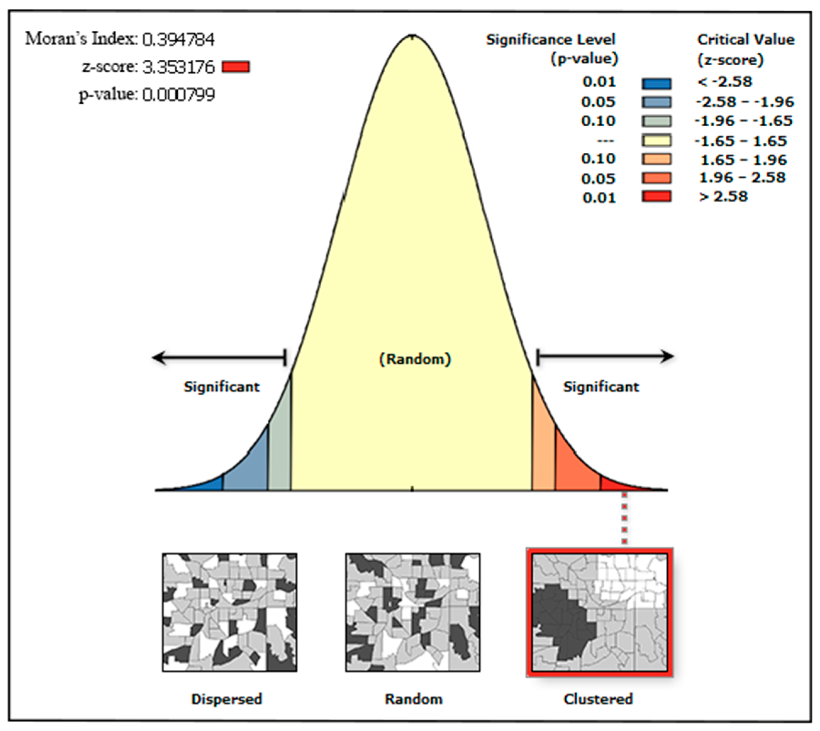
4.2. Spatial Quantitative Analysis of UBD and LST

The results of the comparison between OLS and GWR were obtained by using the GWR module of Arcgis10.3 software. The results are shown in Table 5.
The GWR model had a larger R2 and smaller Akaike information criterion ( A I C c ) and sigma, indicating that the LST and UBD fitting effects based on the GWR model were better than those based on the OLS model. First, according to the GWR regression results, the overall effect of this model is significant, and UBD can explain 54.2% of the LST total variation. In the OLS model, UBD can only explain up to 33.8% of the LST variance. Figure 13a,b shows the residual spatial distributions of OLS and GWR; compared with the results of OLS, the residuals dropped from 43.13 to 27.96. It is not suitable for the global model to be established based on the OLS method because there is a strong spatial correlation. Although spatial autocorrelation still exists in the GWR model residual, it is lower than that in the OLS method and presents a more random spatial distribution.
At the same time, the Akaike information criterion ( A I C c ) of GWR dropped significantly from −717.2 to −1464.9. The A I C c is a measure of the fitting degree to a statistical model. According to the evaluation criteria proposed by Fotheringham, a difference between the two of greater than 3 is the optimal bandwidth, and the lower the value, the better the fitting effect. Even considering the complexity of the GWR, the GWR model is better than the OLS model, and the difference between the two models far exceeds this value.
The spatial distribution of the local fitting result of the GWR model (Local R2) is shown in Figure 14. Where the subsurface of the suburbs is dominated by grassland and cultivated land, the LST is mainly affected by vegetation and the GWR model has a high fitting degree. However, in the central urban area where buildings are concentrated, the LST is affected by the buildings and the fitting degree of the GWR is relatively low.

5. Discussion

In this study, we first estimated the UBD and LST using Luojia1-01 NTL imagery and then used the GWR model in the central city zone of Hefei as an example to study the correlation between the two. The following conclusions were obtained:
(1)
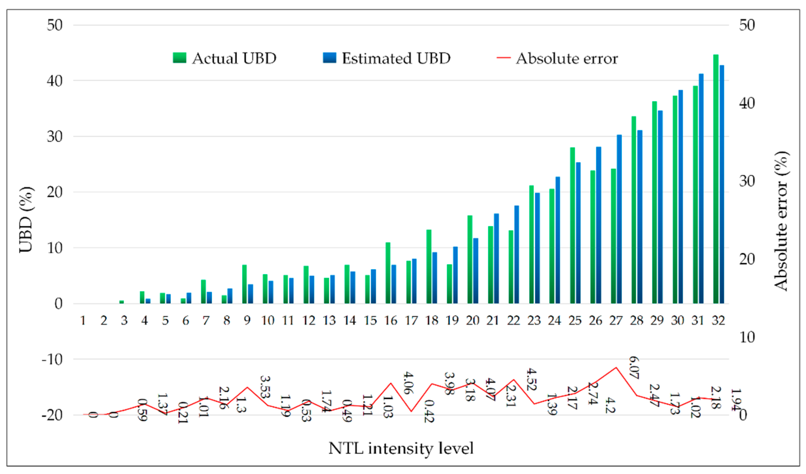
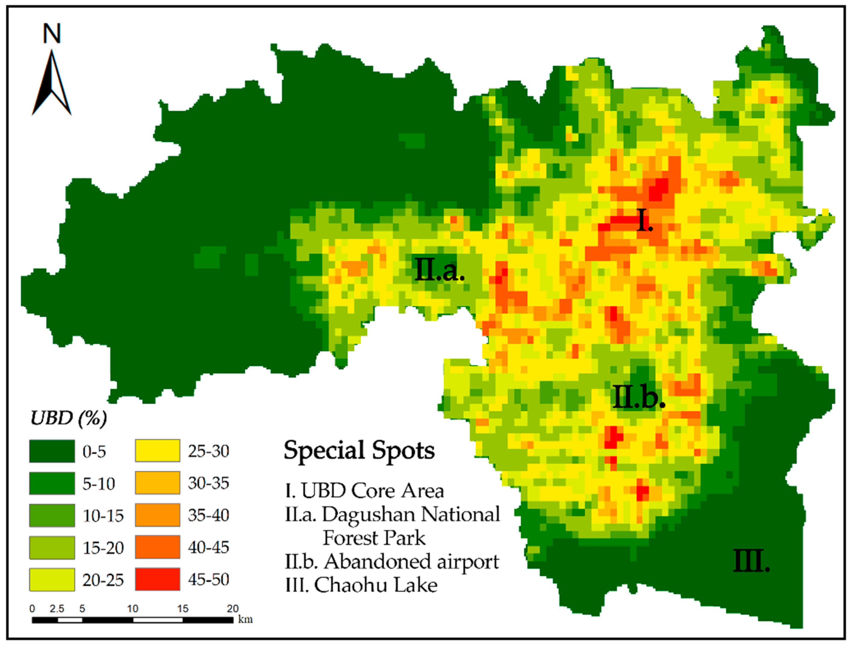
According to the accuracy verification, the absolute error between the estimated and actual values of UBD was only 3.58%, which proves that Luojia1-01 NTL imagery has strong potential for UBD estimation. The UBD can better reflect the aggregation degree in the built-up area of Hefei and is a full expression of urbanization. Its main feature is that UBD decreases from the interior to the periphery. The areas with high UBD are concentrated in the interior. Where the buildings are dense, the UBD index is large and concentrated, while the lower UBD areas are mostly scattered in the outer suburbs with more vegetation.
(2)
UBD and LST were found to be positively spatially correlated at all four scales examined, and the larger the spatial scale, the greater the correlation found.
(3)
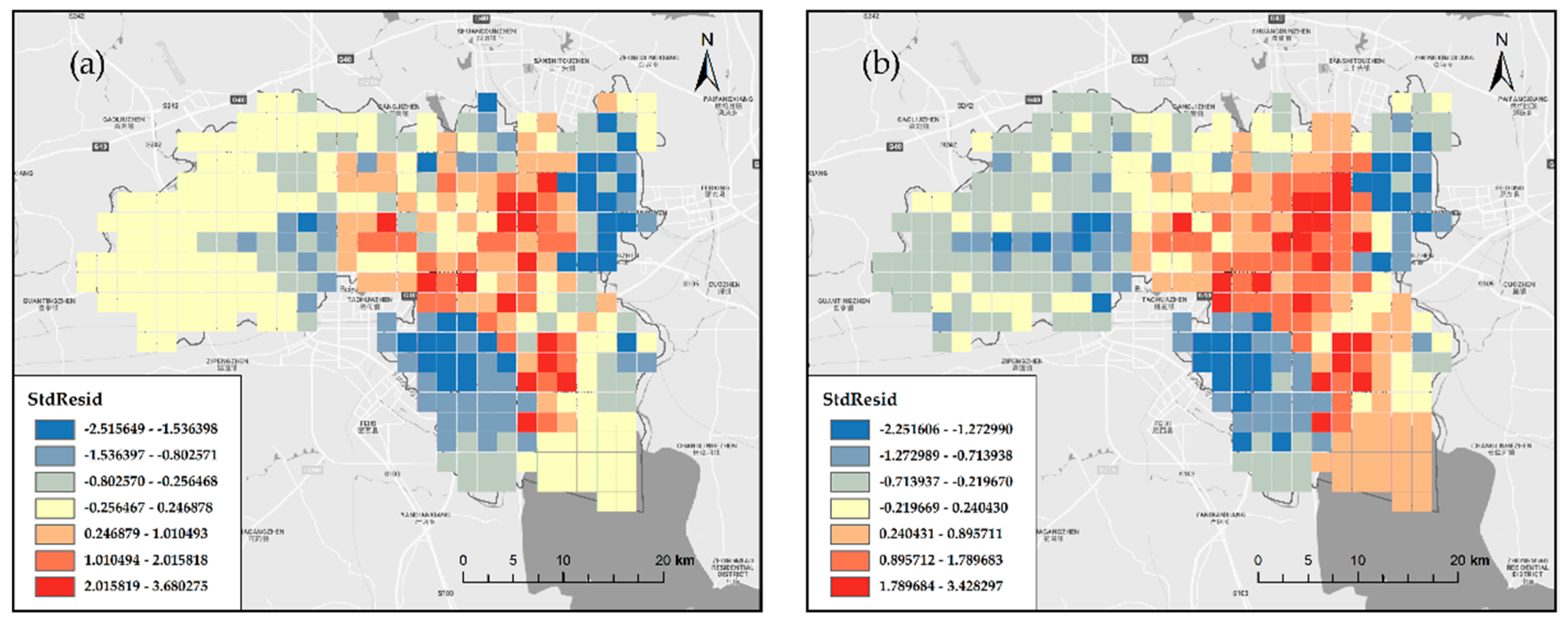
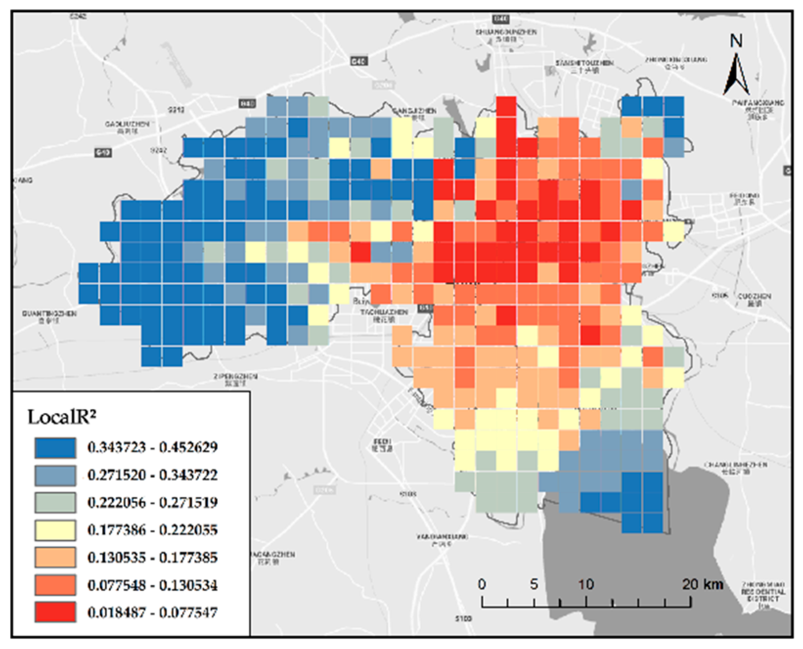
The simulation effect of GWR was significantly better than that of OLS. GWR had the smallest A I C c and Sigma, and the largest R 2, while the regression residual of OLS was higher than that of GWR. OLS overestimated or underestimated the heating or cooling capacity of different UBDs. GWR can well reflect the influence of UBD on the LST in different spatial locations, and the results showed excellent visualization effects. Therefore, when studying the relationship between UBD and LST in the city, GWR is more intuitive and accurate.
The results show that there is a significant correlation between UBD and LST as a whole. The LST was higher in regions with higher UBD, and vice versa. In addition, the GWR’s simulated effect and regression coefficient in the central city were lower than those in the suburbs because the underlying surface of the central city is dominated by buildings, while in the suburbs, vegetation is abundant. This indicates that the LST is more affected by vegetation than by buildings.

6. Conclusions

This paper took the main urban area of Hefei as the research area, used Luojia1-01 NTL imagery to estimate the UBD, and combined this with the Landsat8 data inversion LST to carry out small-scale correlation analysis and modeling.
The emergence of Luojia1-01 NTL imagery opens a new door for microscale research, and it is essential to explore its potential. In this paper, we applied remote sensing image data sourced from Luojia1-01 NTL imagery to the internal research of a city, which proved that it can be used effectively for the extraction of urban information. However, the research still has the following shortcomings: (1) The team at Wuhan University only released the Luojia1-01 NTL data for 2018, so it is hard to perform a multi-time series analysis and we lack a comprehensive evaluation method. (2) Many other factors, such as rainfall, vegetation, and wind speed, also affect LST changes. Future research could integrate more factors into the GWR model for a more detailed analysis. We will strive to improve the reliability and comparability of the Luojia1-01 NTL data estimation results so as to facilitate a more detailed analysis of the heat island distribution pattern and its evolution, which is our future research direction.

Author Contributions

Conceptualization, X.W., and T.Z.; data curation, F.Z.; funding acquisition, T.Z., and F.T.; methodology, X.W., T.Z., and F.T.; project administration, T.Z., and F.T.; software, X.W.; validation, X.W., T.Z., and F.T.; visualization, X.W.; writing—original draft, X.W., T.Z., and F.Z.; writing—review & editing, T.Z., F.T., and F.Z.

Funding

This research was funded by the National Natural Science Foundation of China under Grant 41301514 and Grant 41401456, in part by the Nantong Key Laboratory Project under Grant CP12016005.

Acknowledgments

The authors would like to thank the editor and the anonymous reviewers who provided insightful comments on improving this article and The Hong Kong Polytechnic University for providing the opportunity of academic exchange. The authors also thank the research team at Wuhan University for freely providing the Luojia1-01 night-time light imagery.

Conflicts of Interest

The authors declare no conflicts of interest.

References

  1. Yang, F.; Lau, S.S.Y.; Qian, F. Summertime heat island intensities in three high-rise housing quarters in inner-city Shanghai China: Building layout, density and greenery. Build. Environ. 2010, 45, 115–134. [Google Scholar] [CrossRef]
  2. Coseo, P.; Larsen, L. Accurate characterization of land cover in urban environments: Determining the importance of including obscured impervious surfaces in urban heat island models. Atmosphere 2019, 10, 347. [Google Scholar] [CrossRef]
  3. Manoli, G.; Fatichi, S.; Schläpfer, M.; Yu, K.; Crowther, T.W.; Meili, N.; Burlando, P.; Katul, G.G.; Bou-Zeid, E. Magnitude of urban heat islands largely explained by climate and population. Nature 2019, 573, 55–60. [Google Scholar] [CrossRef]
  4. Liu, Y.; Peng, J.; Wang, Y. Efficiency of landscape metrics characterizing urban land surface temperature. Landsc. Urban Plan. 2018, 180, 36–53. [Google Scholar] [CrossRef]
  5. Wang, R.; Cai, M.; Ren, C.; Bechtel, B.; Xu, Y.; Ng, E. Detecting multi-temporal land cover change and land surface temperature in Pearl River Delta by adopting local climate zone. Urban Clim. 2019, 28, 100455. [Google Scholar] [CrossRef]
  6. Wang, C.; Li, Y.; Myint, S.W.; Zhao, Q.; Wentz, E.A. Impacts of spatial clustering of urban land cover on land surface temperature across Köppen climate zones in the contiguous United States. Landsc. Urban Plan. 2019, 192, 103668. [Google Scholar] [CrossRef]
  7. Zhang, Y.; Sun, L. Spatial-temporal impacts of urban land use land cover on land surface temperature: Case studies of two Canadian urban areas. Int. J. Appl. Earth Obs. Geoinf. 2019, 75, 171–181. [Google Scholar] [CrossRef]
  8. Ghellere, M.; Bellazzi, A.; Belussi, L.; Meroni, I. Urban monitoring from infrared satellite images. Appl. Opt. 2016, 55, 106–114. [Google Scholar] [CrossRef]
  9. He, B.-J. Towards the next generation of green building for urban heat island mitigation: Zero UHI impact building. Sustain. Cities Soc. 2019, 50, 101647. [Google Scholar] [CrossRef]
  10. Liu, H.; Zhan, Q.; Gao, S.; Yang, C. Seasonal variation of the spatially non-stationary association between land surface temperature and urban landscape. Remote Sens. 2019, 11, 1016. [Google Scholar] [CrossRef]
  11. Zhou, Y.; Lin, C.; Wang, S.; Liu, W.; Tian, Y. Estimation of building density with the integrated use of GF-1 PMS and Radarsat-2 data. Remote Sens. 2016, 8, 969. [Google Scholar] [CrossRef]
  12. Guo, F.; Zhu, P.; Wang, S.; Duan, D.; Jin, Y. Improving natural ventilation performance in a high-density urban district: A building morphology method. Procedia Eng. 2017, 205, 952–958. [Google Scholar] [CrossRef]
  13. Yang, X.; Li, Y. The impact of building density and building height heterogeneity on average urban albedo and street surface temperature. Build. Environ. 2015, 90, 146–156. [Google Scholar] [CrossRef]
  14. Zhang, J.; Xu, L.; Shabunko, V.; Tay, S.E.R.; Sun, H.; Lau, S.S.Y.; Reindl, T. Impact of urban block typology on building solar potential and energy use efficiency in tropical high-density city. Appl. Energy 2019, 240, 513–533. [Google Scholar] [CrossRef]
  15. Resch, E.; Bohne, R.A.; Kvamsdal, T.; Lohne, J. Impact of urban density and building height on energy use in cities. Energy Procedia 2016, 96, 800–814. [Google Scholar] [CrossRef]
  16. Amaya-Espinel, J.D.; Hostetler, M.; Henríquez, C.; Bonacic, C. The influence of building density on Neotropical bird communities found in small urban parks. Landsc. Urban Plan. 2019, 190, 103578. [Google Scholar] [CrossRef]
  17. Chan, I.Y.S.; Liu, A.M.M. Effects of neighborhood building density, height, greenspace, and cleanliness on indoor environment and health of building occupants. Build. Environ. 2018, 145, 213–222. [Google Scholar] [CrossRef]
  18. Stewart, I.D.; Oke, T.R.; Krayenhoff, E.S. Evaluation of the “local climate zone” scheme using temperature observations and model simulations. Int. J. Climatol. 2014, 34, 1062–1080. [Google Scholar] [CrossRef]
  19. Perini, K.; Magliocco, A. Effects of vegetation, urban density, building height, and atmospheric conditions on local temperatures and thermal comfort. Urban For. Urban Green. 2014, 13, 495–506. [Google Scholar] [CrossRef]
  20. Yin, C.; Yuan, M.; Lu, Y.; Huang, Y.; Liu, Y. Effects of urban form on the urban heat island effect based on spatial regression model. Sci. Total Environ. 2018, 634, 696–704. [Google Scholar] [CrossRef]
  21. Bonafoni, S.; Keeratikasikorn, C. Land Surface Temperature and Urban Density: Multiyear Modeling and Relationship Analysis Using MODIS and Landsat Data. Remote Sens. 2018, 10, 1471. [Google Scholar] [CrossRef]
  22. Luxmoore, D.A.; Jayasinghe, M.T.R.; Mahendran, M. Mitigating temperature increases in high lot density sub-tropical residential developments. Energy Build. 2005, 37, 1212–1224. [Google Scholar] [CrossRef]
  23. Giridharan, R.; Lau, S.S.Y.; Ganesan, S.; Givoni, B. Urban design factors influencing heat island intensity in high-rise high-density environments of Hong Kong. Build. Environ. 2007, 42, 3669–3684. [Google Scholar] [CrossRef]
  24. Hu, Y.; White, M.; Ding, W. An urban form experiment on urban heat island effect in high density area. Procedia Eng. 2016, 169, 166–174. [Google Scholar] [CrossRef]
  25. Benza, M.; Weeks, J.R.; Stow, D.A.; López-Carr, D.; Clarke, K.C. A pattern-based definition of urban context using remote sensing and GIS. Remote Sens. Environ. 2016, 183, 250–264. [Google Scholar] [CrossRef]
  26. Yao, R.; Wang, L.; Huang, X.; Niu, Y.; Chen, Y.; Niu, Z. The influence of different data and method on estimating the surface urban heat island intensity. Ecol. Indic. 2018, 89, 45–55. [Google Scholar] [CrossRef]
  27. Yu, X.; Guo, X.; Wu, Z. Land surface temperature retrieval from Landsat 8 TIRS—Comparison between radiative transfer equation-based method, split window algorithm and single channel method. Remote Sens. 2014, 6, 9829–9852. [Google Scholar] [CrossRef]
  28. Pan, X.-Z.; Zhao, Q.-G.; Chen, J.; Liang, Y.; Sun, B. Analyzing the variation of building density using high spatial resolution satellite images: The example of Shanghai City. Sensors 2008, 8, 2541–2550. [Google Scholar] [CrossRef]
  29. Huang, X.; Lu, Q.; Zhang, L. A multi-index learning approach for classification of high-resolution remotely sensed images over urban areas. ISPRS J. Photogramm. Remote Sens. 2014, 90, 36–48. [Google Scholar] [CrossRef]
  30. Qi, K.; Hu, Y.n.; Cheng, C.; Chen, B. Transferability of economy estimation based on DMSP/OLS night-time light. Remote Sens. 2017, 9, 786. [Google Scholar] [CrossRef]
  31. Wu, J.; Wang, Z.; Li, W.; Peng, J. Exploring factors affecting the relationship between light consumption and GDP based on DMSP/OLS nighttime satellite imagery. Remote Sens. Environ. 2013, 134, 111–119. [Google Scholar] [CrossRef]
  32. Keola, S.; Andersson, M.; Hall, O. Monitoring economic development from space: Using nighttime light and land cover data to measure economic growth. World Dev. 2015, 66, 322–334. [Google Scholar] [CrossRef]
  33. Ma, T.; Zhou, Y.; Zhou, C.; Haynie, S.; Pei, T.; Xu, T. Night-time light derived estimation of spatio-temporal characteristics of urbanization dynamics using DMSP/OLS satellite data. Remote Sens. Environ. 2015, 158, 453–464. [Google Scholar] [CrossRef]
  34. Xie, Y.; Weng, Q. Spatiotemporally enhancing time-series DMSP/OLS nighttime light imagery for assessing large-scale urban dynamics. ISPRS J. Photogramm. Remote Sens. 2017, 128, 1–15. [Google Scholar] [CrossRef]
  35. Xie, Y.; Weng, Q. Updating urban extents with nighttime light imagery by using an object-based thresholding method. Remote Sens. Environ. 2016, 187, 1–13. [Google Scholar] [CrossRef]
  36. Zhou, T.; Shi, W.; Liu, X.; Tao, F.; Qian, Z.; Zhang, R. A Novel Approach for Online Car-Hailing Monitoring Using Spatiotemporal Big Data. IEEE Access 2019, 7, 128936–128947. [Google Scholar] [CrossRef]
  37. Li, X.; Li, D.; Xu, H.; Wu, C. Intercalibration between DMSP/OLS and VIIRS night-time light images to evaluate city light dynamics of Syria’s major human settlement during Syrian Civil War. Int. J. Remote Sens. 2017, 38, 5934–5951. [Google Scholar] [CrossRef]
  38. Li, X.; Liu, S.; Jendryke, M.; Li, D.; Wu, C. Night-time light dynamics during the Iraqi Civil War. Remote Sens. 2018, 10, 858. [Google Scholar] [CrossRef] [Green Version]
  39. Falchetta, G.; Noussan, M. Interannual variation in night-time light radiance predicts changes in national electricity consumption conditional on income-level and region. Energies 2019, 12, 456. [Google Scholar] [CrossRef] [Green Version]
  40. Xie, Y.; Weng, Q. Detecting urban-scale dynamics of electricity consumption at Chinese cities using time-series DMSP-OLS (Defense Meteorological Satellite Program-Operational Linescan System) nighttime light imageries. Energy 2016, 100, 177–189. [Google Scholar] [CrossRef]
  41. Chen, T.-H.K.; Prishchepov, A.; Fensholt, R.; Sabel, C. Detecting and monitoring long-term landslides in urbanized areas with nighttime light data and multi-seasonal Landsat imagery across Taiwan from 1998 to 2017. Remote Sens. Environ. 2019, 225, 317–327. [Google Scholar] [CrossRef]
  42. Mohamadi, B.; Chen, S.; Liu, J. Evacuation priority method in tsunami hazard based on DMSP/OLS population mapping in the Pearl River Estuary, China. ISPRS Int. J. Geoinf. 2019, 8, 137. [Google Scholar] [CrossRef] [Green Version]
  43. Jiang, W.; He, G.; Long, T.; Guo, H.; Yin, R.; Leng, W.; Liu, H.; Wang, G. Potentiality of using Luojia 1-01 nighttime light imagery to investigate artificial light pollution. Sensors 2018, 18, 2900. [Google Scholar] [CrossRef] [PubMed] [Green Version]
  44. Li, X.; Zhao, L.; Li, D.; Xu, H. Mapping urban extent using Luojia 1-01 nighttime light imagery. Sensors 2018, 18, 3665. [Google Scholar] [CrossRef] [PubMed] [Green Version]
  45. Ou, J.; Liu, X.; Liu, P.; Liu, X. Evaluation of Luojia 1-01 nighttime light imagery for impervious surface detection: A comparison with NPP-VIIRS nighttime light data. Int. J. Appl. Earth Obs. Geoinf. 2019, 81, 1–12. [Google Scholar] [CrossRef]
  46. Zhang, G.; Guo, X.; Li, D.; Jiang, B. Evaluating the potential of LJ1-01 nighttime light data for modeling socio-economic parameters. Sensors 2019, 19, 1465. [Google Scholar] [CrossRef] [Green Version]
  47. Li, C.; Zou, L.; Wu, Y.; Xu, H. Potentiality of using Luojia1-01 night-time light imagery to estimate urban community housing price—A case study in Wuhan, China. Sensors 2019, 19, 3167. [Google Scholar] [CrossRef] [Green Version]
  48. Zhong, X.; Su, Z.; Zhang, G.; Chen, Z.; Meng, Y.; Li, D.; Liu, Y. Analysis and reduction of solar stray light in the nighttime imaging camera of Luojia-1 satellite. Sensors 2019, 19, 1130. [Google Scholar] [CrossRef] [Green Version]
  49. Liu, M.; Cao, C.; Chen, W.; Wang, X. Mapping canopy heights of poplar plantations in plain areas using ZY3-02 stereo and multispectral data. ISPRS Int. J. Geoinf. 2019, 8, 106. [Google Scholar] [CrossRef] [Green Version]
  50. Hormese, J.; Saravanan, C. Automated road extraction from high resolution satellite images. Procedia Technol. 2016, 24, 1460–1467. [Google Scholar] [CrossRef] [Green Version]
  51. Fu, Z.; Sun, Y.; Fan, L.; Han, Y. Multiscale and Multifeature Segmentation of High-Spatial Resolution Remote Sensing Images Using Superpixels with Mutual Optimal Strategy. Remote Sens. 2018, 10, 1289. [Google Scholar] [CrossRef] [Green Version]
  52. Bakhtiari, H.R.R.; ABDollahi, A.; Rezaeian, H. Semi automatic road extraction from digital images. Egypt. J. Remote Sens. Space Sci. 2017, 20, 117–123. [Google Scholar] [CrossRef]
  53. Mena, J.B. State of the art on automatic road extraction for GIS update: A novel classification. Pattern Recognit. Lett. 2003, 24, 3037–3058. [Google Scholar] [CrossRef]
  54. Ma, X.; Longley, I.; Gao, J.; Kachhara, A.; Salmond, J. A site-optimised multi-scale GIS based land use regression model for simulating local scale patterns in air pollution. Sci. Total Environ. 2019, 685, 134–149. [Google Scholar] [CrossRef]
  55. Zhang, L.; Gove, J.H.; Heath, L.S. Spatial residual analysis of six modeling techniques. Ecol. Model. 2005, 186, 154–177. [Google Scholar] [CrossRef]
  56. Lou, M.; Zhang, H.; Lei, X.; Li, C.; Zang, H. Spatial autoregressive models for stand top and stand mean height relationship in mixed quercus mongolica broadleaved natural stands of northeast China. Forests 2016, 7, 43. [Google Scholar] [CrossRef] [Green Version]
  57. Sun, Y.; Gao, C.; Li, J.; Wang, R.; Liu, J. Quantifying the effects of urban form on land surface temperature in subtropical high-density urban areas using machine learning. Remote Sens. 2019, 11, 959. [Google Scholar] [CrossRef] [Green Version]
Figure 1. The changes in area of each land type of Hefei during the past 15 years.
Applsci 09 05224 g001
Figure 2. The study area.
Applsci 09 05224 g002
Figure 3. Remote sensing image data of the study area: (a) Night light image from Luojia1-01; (b) Standard false-color composite images (made up of information from Bands 3–5) from Landsat8, where the vegetation is red, the waterbody is blue, and the white is roads and buildings; and (c) ZY3-02 Multi-spectral image from ZY3-02, where the vegetation is green, the waterbody is white, and the gray is buildings and roads.
Applsci 09 05224 g003
Figure 4. Schematic diagram of plots and example of building digitalization: (a) Urban building density (UBD) sample area distribution; (b) Example of a sample area; and (c) Example of building digitization in a sample area.
Applsci 09 05224 g004
Figure 5. Flowchart of the procedure for eliminating the interference of road lighting in the Luojia1-01 images.
Applsci 09 05224 g005
Figure 6. Scatter diagrams of the polynomial fitting results of the actual UBD and night-time light (NTL) of the 320 sample areas: (a) Before stripping the road area; and (b) After stripping the road area.
Applsci 09 05224 g006
Figure 7. Relation of UBD and the Luojia1-01 NTL value.
Applsci 09 05224 g007
Figure 8. Statistical chart of the average UBD fitting results of samples of various classes of NTL intensity.
Applsci 09 05224 g008
Figure 9. A sketch map of the overall UBD distribution in the study area.
Applsci 09 05224 g009
Figure 10. A sketch map of the overall LST distribution in the study area.
Applsci 09 05224 g010
Figure 11. Correlation between LST and UBD at four spatial scales: (a) UBD—LST at 0.5 km; (b) UBD—LST at 1 km; (c) UBD—LST at 1.5 km; and (d) UBD—LST at 2 km.
Applsci 09 05224 g011
Figure 12. Schematic diagram of Moran’s I analysis of the LST in the study area.
Applsci 09 05224 g012
Figure 13. Schematic diagram of standard residuals for UBD and LST: (a) Standard residual plot of OLS; and (b) Standard residual plot of GWR.
Applsci 09 05224 g013
Figure 14. Schematic diagram of the local fitting results of the GWR model for UBD and LST.
Applsci 09 05224 g014
Table 1. The UBD levels in the study area.
Density ClassDensity Range/%Area Percent/%
low0–538.77
5–108.29
sub-low10–154.34
15–2010.66
middle20–2513.01
25–3011.59
sub-high30–355.86
35–403.11
high40–452.58
45–501.79
Table 2. UBD sampling results in the study area.
Test SampleAverage NTLActual UBD (%)Estimated UBD (%)Absolute Error (%)
10.03494030.2436.635.29
20.0010090.520.570.05
316.68363916.9719.22.23
40.0084499.0813.574.49
50.03729927.2438.1710.93
60.0036762.320.022.3
70.000039000
80.0057667.034.482.55
90.02040617.2423.15.86
100.0025322.831.361.47
110.04367530.5239.258.73
120.0111928.0914.025.93
130.0098379.4313.584.15
140.00859410.3517.377.02
150.000065000
160.0049964.572.322.25
170.02742420.1331.8711.74
180.0030962.951.621.33
190.0077937.5213.936.41
200.02262722.0229.467.44
average11.4515.033.58
Table 3. Inversion accuracy verification of LST.
Data SourcesMaximum (°C)Minimum (°C)Average (°C)Standard Deviation (°C)
RTE inversion value36.9312.0627.444.72
MOD11A1 data34.0715.6226.31
Table 4. Temperature grading basis and temperature intervals.
Temperature ClassGrading BasisTemperature Range/°CArea Percent/%
low μ S D > T T < 23.069.04%
sub-low μ 0.5 S D > T μ S D 23.06 ≤ T < 26.9733.87%
middle μ + 0.5 S D > T μ 0.5 S D 26.97 ≤ T ≤ 30.8821.11%
sub-high μ + S D > T μ + 0.5 S D 30.88 < T ≤ 34.9325.77%
high T μ + S D T > 34.9310.21%
Table 5. Simulation effect by Geographically Weighted Regression (GWR) and a comparison with ordinary least squares (OLS).
AIC c R adj 2 SigmaResidual
OLS−717.20.3382.23743.13
GWR−1464.90.5421.75327.96

