Article

A Shearlets-Based Method for Rain Removal from Single Images

1
School of Mathematical Sciences, University of Electronic Science and Technology of China, Chengdu 610054, China
2
Engineering School, DEIM, University of Tuscia, 01100 Viterbo, Italy
*
Authors to whom correspondence should be addressed.
Appl. Sci. 2019, 9(23), 5137; https://doi.org/10.3390/app9235137
Submission received: 21 October 2019 / Revised: 14 November 2019 / Accepted: 21 November 2019 / Published: 27 November 2019

Abstract

:

Featured Application

The Shearletes-based rain removal method proposed in this paper can be applied to the destriping of remote sensing images and removing other directional noises.

Abstract

This work focuses on the problem of rain removal from a single image. The directional multilevel system, Shearlets, is used to describe the intrinsic directional and structure sparse priors of rain streaks and the background layer. In this paper, a Shearlets-based convex rain removal model is proposed, which involves three sparse regularizers: including the sparse regularizer of rain streaks and two sparse regularizers of the Shearlets transform of background layer in the rain drops’ direction and the Shearlets transform of rain streaks in the perpendicular direction. The split Bregman algorithm is utilized to solve the proposed convex optimization model, which ensures the global optimal solution. Comparison tests with three state-of-the-art methods are implemented on synthetic and real rainy images, which suggests that the proposed method is efficient both in rain removal and details preservation of the background layer.

1. Introduction

Rain removal from a single image is an important issue in processing outdoor vision problems. In fact, the outdoor images are often degraded by the rain streak and other bad weather conditions, and these bad weather conditions can lead to the change of local or global intensities and color contrast in real images, thus causing unclear visible scenes. Such degradation severely affects the performance of algorithms in computer vision systems. Therefore, the removal of rain streaks is essential.
In recent years, the rain removal problem has caused more and more attention. There are many approaches for rain removal using different modelings. They can be classified into two kinds, including the video-based methods and the single image-based methods. In fact, there are many literatures for the video-based methods [1,2,3,4,5,6,7,8,9,10], the main idea is taking advantage of the rich detail of multiple relative images and the similarity of the image sequences to detect rain streaks and recover the background layer. For instance, Garg and Nayar [1] proposed a correlation model to capture the dynamics of rain in video, then removed rain streaks by a physics-based motion blur model. That is, once rain streaks are detected, the corresponding pixel value of rain is obtained by averaging the rain-free temporal neighbors. In [4], Garg and Nayar found that the video rain visibility relies heavily on the exposure time and the depth of field, based on this fact, they introduced a self-adaption parameter model to remove rain streaks efficiently. In addition, Zhang in [2] gives a new rain removal model, which is based on two priors, one is rain streaks that are almost the same in RGB channels and the other is rain streaks that do not appear everywhere in video. Recently, Jiang et al. proposed a novel tensor-based video rain streaks removal approach via utilizing discriminatively intrinsic priors in [10], by fully considering the discriminatively intrinsic characteristics of rain streaks and clean videos, which needs neither rain detection nor time-consuming dictionary learning stage. This method is based on the following priors, including that rain streaks are sparse and smooth in the rain-drop direction and the clean video is smooth along the rain-perpendicular direction, which are both global and local correlation in time direction.
For the single images-based methods, it is more difficult than video-based method due to the limited single image information, thus there are fewer works for single image rain removal. The most successful methods are given in literatures [11,12,13,14,15,16,17,18,19,20,21]. For instance, in [11], based on the assumption that a rainy image can be represented by the rain layer and the background layer, the author proposed a dictionary learning method-based nonlinear screen blend model for rain removal from single images. The key for this method is that by sparse coding of two layers using the sparse dictionary, by learning sparse dictionary, the accurate layer decompositions are obtained. Moreover, in [14], Kang et al. decomposed the rainy image into low frequency and high frequency parts, and applied an MCA-based dictionary learning model to split the rain streaks layer in the high frequency domain. Following this idea, the author in [16] introduced the structure information into consideration, but the estimated background layer tends to be blurry. Then Li et al. gives another additional model in [13], which is a linear super-imposition of the desired background layer and the rain streak layer, which is an energy minimization model, and the Gaussian mixture model is utilized to learn the corresponding patch-based priors for two layers. The advantage of this model is that it can detect different orientations and scales of the rain streak, which leads to state-of-the-art rain removal results. In fact, these methods described above do remove the rain streaks from rainy images, but the recovery of background seems to be over-smoothed, that is, some details of the background layer are lost. The main reason for details missing in general methods is that the directional property of two layers is out of consideration, which is critical in edges detection. Based on this fact, the author in [21] proposed a directional global sparse model for single image rain removal, in this work, undirectional total removal (UTV) [22] is introduced to describe the basic directional property of single rainy images. The proposed optimization model is based on two directional sparse priors of rain streaks and background layer respectively and a generally sparse prior on rain streaks, that is, rain streaks are sparse in the vertical direction, while the rain-free image (background layer) is sparse in the horizontal direction; furthermore, the rain streak is approximately considered as sparse when the rain is not heavy. The directional characters are captured by rotating rainy images appropriately, which ensures that rain streaks are mainly concentrated in the vertical direction.
In addition, the deep learning-based method gives another way for single image and video rain removal [23,24,25,26], which is totally different from the traditional image processing. The key for this approach is the training network. By learning from lots of rainy images, the learning model can split rain streaks from rainy images after thousands of training images, which is time-consuming, but once the training model gets good generalization, it can deal with lots of rainy images simultaneously, with an accuracy of at least 80 percent. With the development of deep learning, the accuracy for splitting rain streaks can be improved further, and this approach will be widely used for other image processing and computer vision tasks.
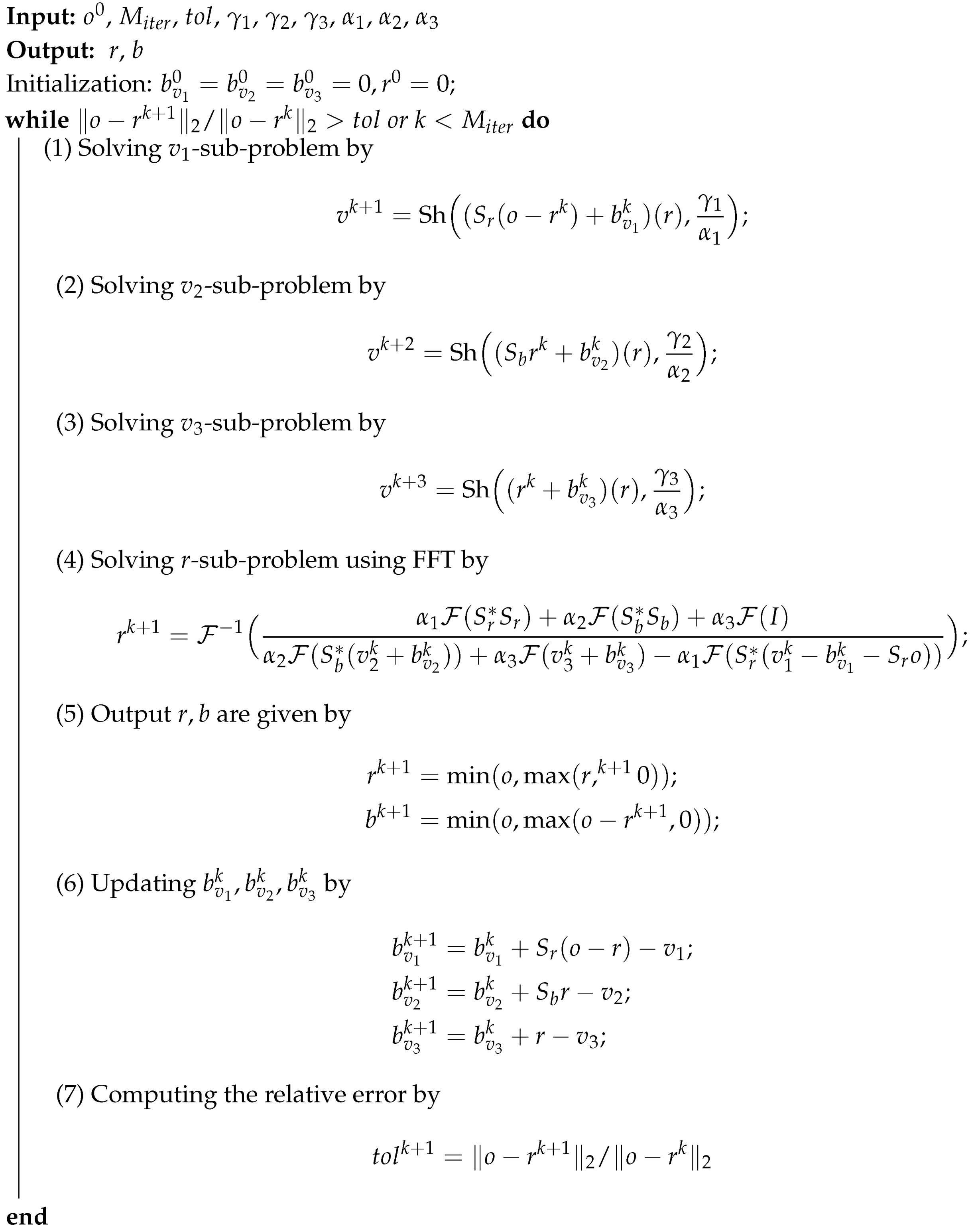
In this work, we consider removing rain streaks from single rainy images. This is different from the method in [21], which removes directional rain streaks by rotating the rainy image to the direction that rain streaks are approximately distributed in the vertical direction, then UTV is utilized to capture the ‘vertical’ characteristics of rain streaks. This is a two-step method when the rain drops are in a non-vertical direction. In fact, directional multilevel transform, e.g., Shearlets transform, can be used to substitute the two-step transform above due to its multi-direction property, also the multilevel system is suitable for detecting rain streaks as the shape of rain streaks is not necessarily rectangular. In addition, we found that the Shearlets decomposition coefficients of rainy images in specific scale and directional frequency bands are sparse. Some statistical analysis (see Figure 1) suggests that the Shearlets coefficients of rainy images in the rain drops’ direction has sparse structure, also the Shearlets coefficients of rain-free (background) layer in the rain streaks direction is sparse. Moreover, another sparse prior is the rain streaks itself, which can be approximately considered as sparse when the rain is not heavy (partly sparse when the rain is heavy). Combining these three sparse priors above, we propose a convex optimization model and the split Bregman algorithm [27] is utilized to solve the proposed model. Numerical experiments on synthetic and real rainy images demonstrate that our Shearlets-based method outperforms the recently widely used rain removal methods in [11,13,21].
The outline of this paper is given as follows: Section 2 gives a brief introduction of the motivation. Section 3 reviews the Shearltes transform. In Section 4, a Shearlets-based rain streaks removal model, and the corresponding algorithm, are proposed. Section 5 compares our model with three state-of-art methods, some discussions of rain removal results are given in Section 6. In the end, the conclusion is given in Section 7.

2. Motivations of the Proposed Method

In general, the rain streak removal model can be represented as follows:
o = r + b ;
where o R M × N is the rainy image, r R M × N represents rain streaks layer, and b R M × N is the background layer (rain-free layer).
Motivated by the work in [14], which decomposed rainy images into high- and low-frequency, then the high-frequency parts can be represented by the addition of rain streaks layer and rain-free layer by performing dictionary learning and sparse coding. This method does remove rain streaks from the rainy image, but the rain-free layer estimated tends to be blurry, which implies that the high-frequency decomposition leads to the loss of details in high frequency not only from rain streaks, but also from the details of the background layer. This makes us consider splitting rain streaks in specific frequency bands, so that more details can be preserved. Therefore, the directional multilevel transform, such as Shearlets transform, is a good choice as it can be used to separate the frequency bands of rain streaks only.
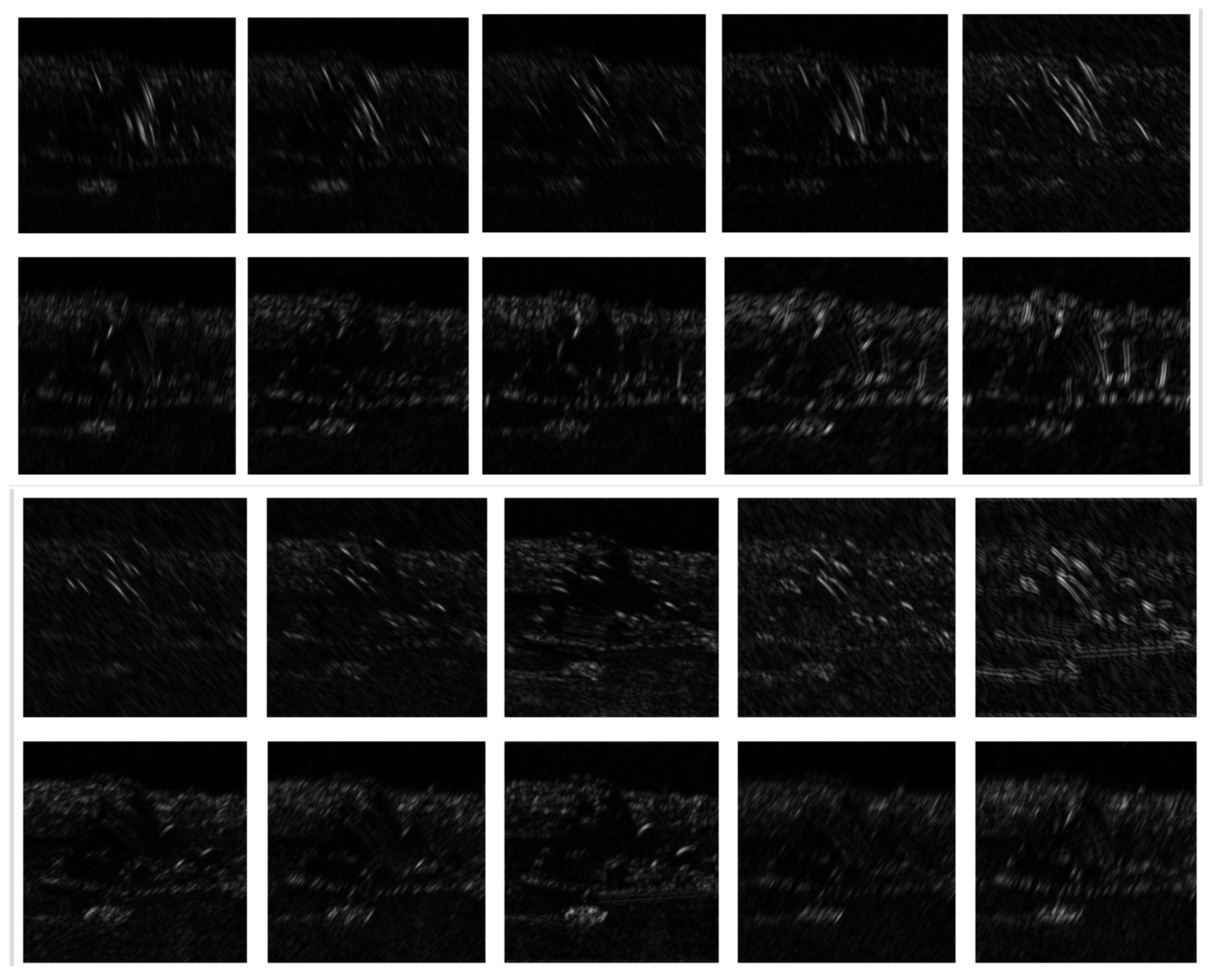
In fact, the Shearlets transform is a powerful tool in detecting directional singularities in frequency band [28,29,30]. Different from UTV, which is used to enforce the sparse prior of the gradient along vertical and horizontal directions, the Shearlets can be utilized to describe the variation along different directions in various scales (see Figure 2). Since the rain streaks can be viewed as a particular directional singularity in different scales, which makes it possible to remove from the rainy image without additional details missing. However, loss of the details from the rain-free layer in corresponding frequency bands cannot be avoided. In order to minimize this kind of details loss, the multi-direction Shearlets is used to preserve most original image details.
Compared with the recent state-of-the-art directional UTV rotation-based rain removal model in [21], the proposed model has the following advantages:
-
The directional multilevel transform, Shearlets transform, is utilized to describe the sparse structure of rain streaks and the background layer. Different from the rotation UTV method, the Shearlets-based method can obtain the gradient variation in different directions and different scales efficiently, thus the recovery keeps more directional singularities details.
-
For different directions of rain streaks, the Shearlets transform can capture the rain streak layer details due to its multi-direction property. Moreover, the fast algorithm for solving the proposed model can be obtained as the discrete Shearlets transform and inverse are available.
-
The split Bregman algorithm is utilized to solve the proposed convex optimization model, which guarantees that the solver is global optimal. The computation of algorithm includes three soft-thresholding processes and two Shearlets transforms, and the total computing complexity is O ( N log N ) + O ( N ) , where N is the total number of pixels.

3. Shearlets

Shearlets system is first given in [31] by Kutyniok et al, which not only inherits the multiscale structure of wavelets, but also possesses the directional windows in the frequency domain by introducing the shear operator, thus making it possible for the Shearlets transform to capture the directional singularities in images and high dimensional signals. This section gives a retrospection of the basic definition and construction of Shearlets, for more details refer to [28,32].
For the basic wavelet function ϕ L 2 ( R 2 ) , it is supposed to satisfy
C ϕ = R 2 | ϕ ^ ( ω ) | 2 | ω | d ω < ,
where ϕ ^ represents the Fourier transform of ϕ , and it has the following separated form:
ϕ ^ ( ω 1 , ω 2 ) = ϕ ^ 1 ( ω 1 ) ϕ ^ 2 ( ω 2 ω 1 ) ,
with ϕ 1 L 2 ( R ) , ϕ 2 L 2 ( R 2 ) . Then the Shearlets multilevel system S is generated by
S ( ϕ ) = { ϕ j , s , t = T t D 2 j S s ϕ : j Z , s R , t R 2 } ,
where T t is the translation operator, T t ϕ = ϕ ( · t ) . D s is the scaling operator and S s is the shear operator, their definitions are given as
D 2 j = 2 j 0 0 2 j / 2 , S s = 1 s 0 1 .
where j Z is the scaling parameter, which decides the decomposition layer. s R is the shearing parameter, which decides the multi-direction property. t is the translation parameter, which decides the number of sub-bands in each scale. For the signal f L 2 ( R 2 ) , its continuous Shearlets transform
f S ( ϕ ) f ( j , s , t ) = < f , ϕ j , s , t > , j Z , s R , t R 2 ,
where S maps f into the Shearlets coefficients S ( ϕ ) f ( j , s , t ) with different scale j, shearing s, and translation t. Then the discrete Shearlets system can be given as
Definition 1
([28]). Let ψ , ϕ L 2 ( R 2 ) , c = ( c 1 , c 2 ) R 2 , the definition of the discrete Shearlets system S ( ψ , ϕ ; c ) is
S ( ψ , ϕ ; c ) = Ψ ( ψ ; c ) Φ ( ϕ ; c ) Φ ˜ ( ϕ ˜ ; c ) ,
where
Ψ ( ψ ; c ) = { ψ j , m = T t D 2 j ψ = 2 3 / 4 ψ ( D 2 j · c m ) : m Z 2 } , Φ ( ϕ ; c ) = { ϕ j , k , m = 2 3 / 4 ϕ ( S k D 2 j · c m ) : j 0 , | k | 2 j / 2 , m Z 2 } , Φ ˜ ( ϕ ˜ ; c ) = { ϕ ˜ j , k , m = 2 3 / 4 ϕ ˜ ( S k D 2 j · c m ) : j 0 , | k | 2 j / 2 , m Z 2 } .
with ψ ^ = ϕ ^ 1 ( ω 1 ) ϕ ^ 2 ( ω 2 ) , and ϕ ˜ ( ξ 1 , ξ 2 ) = ϕ ( ξ 2 , ξ 1 ) .
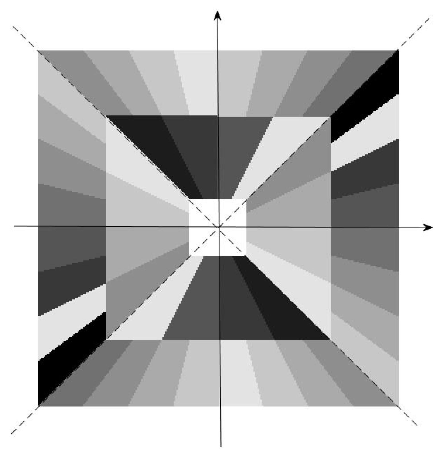
The multilevel system Ψ ( ψ ; c ) corresponds to the low frequency area in the frequency domain, while the system Φ ( ϕ ; c ) and Φ ˜ ( ϕ ˜ ; c ) corresponds to the high frequency region in vertical and horizontal direction respectively. The sub-band of S ( ψ , ϕ ; c ) in the frequency domain is shown in Figure 3.

4. The Proposed Method

4.1. The Proposed Optimization Model

This subsection describes the proposed convex model with three sparse prior regularizers and some non-negative constraints as follows:
  • The sparse constraint of the Shearets coefficients of the background layer in the rain drops’ direction. In fact, the Shearlets decomposition coefficients of the background layer in high frequency can be approximately considered (in the rain drops’ direction) as sparse (see Figure 1) due to the intensity distribution for multilevel coefficients. In order to describe this sparse regularizer, the 1 norm of multilevel coefficients in different scales, along the direction of the rain-free layer is used, which also reflects the discontinuity of rain streaks, specifically
    R e g 1 ( b ) = S r b 1 = S r ( o r ) 1 ;
    where S r b is the Shearlets transform of the rain-free layer in the rain drops’ direction.
  • The sparse constraint of the Shearlets coefficients of the rain streaks across the rain drops’ direction. In the real scenes of rainfall, the shape of rain streaks is a stretched ellipse in a specific direction reflected in pixels, therefore the directional multilevel transform is more sensitive than UTV in detecting the directional singularities in images. From Figure 2, it shows that the Shearlets coefficient in scale 2 across the rain drops’ direction of the rain streak has sparse structure. Similarly,
    R e g 2 ( r ) = S b r 1 .
    where S b r is the Shearlets transform of the rain streak across the rain drops’ direction.
  • The sparse constraint of rain streaks (see Figure 1). In general, the rain streak is sparse when the rain is not heavy, therefore its sparsity can be described by 0 norm, which represents the number of nonzero elements. Here, the 1 is utilized to replace the 0 norm due to its non-convexity, thus we have the following sparse regularizer of rain streaks
    R e g 3 ( r ) = r 1 .
  • Some non-negative constraints of r and b. For the rain streaks removal problem, the pixel of the rain streaks layer r and the background layer b are non-negative, therefore the following constraints hold
    C o n 1 ( r , b ) : r 0 ; b 0 .
By analyzing the property of multi-direction Shearlets transform of rain streaks and background layers, the corresponding sparse regularizers are obtained. With constraints of r and b, the optimization model for solving single image rain removal problem can be given as follows:
min s γ 1 S r ( o r ) 1 + γ 2 S b r 1 + γ 3 r 1 , s . t . r 0 ; b 0 ;
where γ i , i = 1 , 2 , 3 are positive regularization parameters. The convexity of (13) guarantees its solver to be global optimal.

4.2. Solving the Proposed Model

To solve the proposed model, the split Bregman algorithm is utilized [27], and the split step is implemented by introducing new variables:
v 1 v 2 v 3 = S r ( o r ) S b r r
as the 1 -norm is not differentiable, thus (13) has the following equivalent form
min γ 1 v 1 1 + γ 2 v 2 1 + γ 3 v 3 1 s . t . v 1 = S r ( o r ) , v 2 = S b r , v 3 = r ; r 0 ; b 0 ;
for non-negative constrains of r and b, they can be implemented by a projection operator. The corresponding Bregman iterations can be given as
( v 1 k + 1 , v 2 k + 1 , v 3 k + 1 , r k + 1 ) = arg min v 1 , v 2 , v 3 , r γ 1 v 1 1 + γ 2 v 2 1 + γ 3 v 3 1 + α 1 2 S r ( o r ) v 1 b v 1 k 2 2 + α 2 2 S b r v 2 b v 2 k 2 2 + α 3 2 r v 3 b v 3 k 2 2 ; b v 1 k + 1 = b v 1 k + S r ( o r ) v 1 ; b v 2 k + 1 = b v 2 k + S b r v 2 ; b v 3 k + 1 = b v 3 k + r v 3 ;
Then the v i -sub-problem i = 1 , 2 , 3 can be given as
v 1 k + 1 = arg min v 1 γ 1 v 1 1 + α 1 2 S r ( o r ) v 1 b v 1 k 2 2 ; v 2 k + 1 = arg min v 2 γ 2 v 2 1 + α 2 2 S b r v 2 b v 2 k 2 2 ; v 3 k + 1 = arg min v 3 γ 3 v 3 1 + α 3 2 r v 3 b v 3 k 2 2 ;
they can be solved accurately by soft-thresholding strategy as follows
v 1 k + 1 = Sh ( S r ( o r k ) + b v 1 k ) ( r ) , γ 1 α 1 ; v 2 k + 1 = Sh ( S b r k + b v 2 k ) ( r ) , γ 2 α 2 ; v 3 k + 1 = Sh ( r k + b v 3 k ) ( r ) , γ 3 α 3 ;
for r = 1 , , N , N represents the total number of pixels, where
Sh ( x , y ) = sign ( x ) max ( | x | y , 0 ) ;
with
sign ( x ) = 1 , x > 0 ; 0 , x = 0 ; 1 , x < 0 .
The r-sub-problem can be given by minimizing the following equation
r k + 1 = arg min r α 1 2 S r ( o r ) v 1 k b v 1 k 2 2 + α 2 2 S b r v 2 k b v 2 k 2 2 + α 3 2 r v 3 k b v 3 k 2 2 ,
since the 2 norm is differentiable, we have the following closed-form solver for r-sub-problem
( α 1 S r * S r + α 2 S b * S b + α 3 I ) r = α 2 S b * ( v 2 k + b v 2 k ) + α 3 ( v 3 k + b v 3 k ) α 1 S r * ( v 1 k b v 1 k S r o ) ,
where I is the identity matrix. From [28], the Shearlets transform is constructed to be a Parseval frame, which implies that S r * S r = I , then the r-sub-problem above can be solved by Fast Fourier Transform (FFT, F ) efficiently.
r k + 1 = F 1 α 1 F ( S r * S r ) + α 2 F ( S b * S b ) + α 3 F ( I ) α 2 F ( S b * ( v 2 k + b v 2 k ) ) + α 3 F ( v 3 k + b v 3 k ) α 1 F ( S r * ( v 1 k b v 1 k S r o ) ) ,
where F 1 represents the Fast Inverse Fourier Transform.
In the end, the constrains for r 0 and b 0 can be projected by the following formula:
r k + 1 = min ( o , max ( r k + 1 , 0 ) ) ; b k + 1 = min ( o , max ( o r k + 1 , 0 ) ) ;
Having explained the main idea of our method, the final resulting algorithm is displayed in Algorithm 1.
Algorithm 1: The split Bregman algorithm for proposed model (13)
Applsci 09 05137 i001

5. Numerical Experiments

In this section, some comparison tests are performed to validate the effectiveness of the proposed method. We compare the proposed method with three recent state-of-art rain removal methods, including a dictionary learning-based algorithm in [11] (15ICCV), a minimization model with the learned rain layer prior method in [13] (16CVPR), and a directional global sparse model in [21] (18UTV). All tests are implemented in a laptop, CPU: Inter Core i5, memory: 16 GB, OS: Windows 10, testing software: Matlab R2016a.
Since humans are more sensitive to changes in luminance, all the RGB testing images are converted to YUV space. The proposed method is utilized to remove rain streaks only in the luminance channel (three compared methods are also implemented on the luminance channel). To be more persuasive, we use two kinds of data for experiments, the synthetic data, and real data. For the synthetic data, the relative error (RelErr), peak signal–noise ration (PSNR), and the structural similarity (SSIM) [33] are used to estimate the performance of different methods.
  • The relative error (RelErr) is defined as
    RelErr = u u r F 2 u F 2 ,
    where u and u r are the original signal and the recovered signal, and · F represents the Frobenius norm.
  • The peak signal–noise ration (PSNR) is defined as
    PSNR = 10 log M N u m a x 2 MSE ,
    where u m a x is the maximum value of u, and
    MSE = 1 M N i = 1 M j = 1 N u ( i , j ) u r ( i , j ) F 2 ,
    where M, N are the size of the signal u.
  • The structural similarity (SSIM) is defined as
    SSIM = ( 2 μ u μ u r + c 1 ) ( 2 σ u u r + c 2 ) ( μ u 2 + μ u r 2 + c 1 ) ( σ u 2 + σ u r 2 + c 2 ) ,
    where μ u and μ u r represent the average of u and u r , σ u , and σ u r represent the standard deviation of u and u r , σ u u r is the covariance of u, and u r , c 1 , c 2 > 0 .

5.1. Comparison Tests of the Synthetic Data

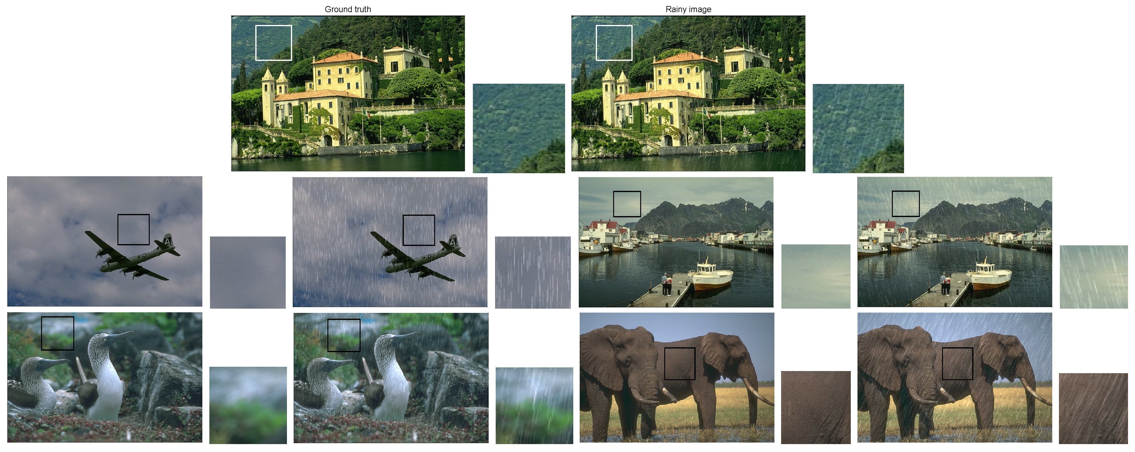
The testing results and discussions for synthetic data are given in this subsection. First, the synthetic rainy image is generated as follows: (1) adding the salt and pepper noise with a random density d e n (which decides the density of rain streaks) to a zero matrix; (2) convoluting (1) with a motion kernel (including the directional parameter θ and motion parameter l e n ); (3) adding (2) to the rain-free images to obtain the rainy image [14]. The parameters of synthetic rainy image for testing are given in Table 1. Then these RGB rainy images are converted to YUV channels, and only the rain streaks in the Y channel are removed using the 15ICCV method, the 16CVPR method, the 18UTV method, and the proposed method. In this test, we choose 5 images as the testing images, which can be downloaded from the dataset “UCID” (http://homepages.lboro.ac.uk/cgs/datasets/ucid/ucid.html) and (https://pixabay.com/).
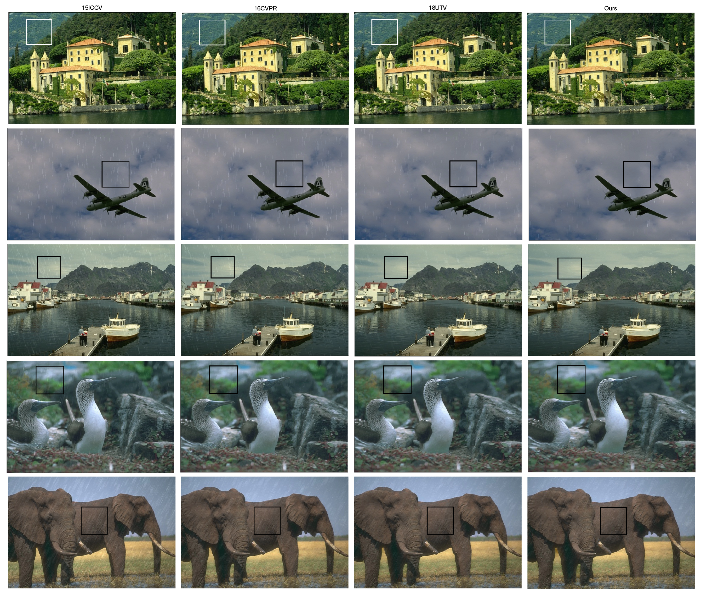
The testing image are given in Figure 4. The visual results for 4 methods are displayed in Figure 5. The first column displays the de-rain results by the 15ICCV method, the second column shows the de-rain results by the 16CVPR method, the third column gives the de-rain results by the 18UTV method, and the last column shows the de-rain results by the proposed method.
From Figure 5 and the corresponding zooming in images in Figure 6, we find that the method 15ICCV fails to remove the rain streak completely, which leads to the lower SSIM value, and while methods 16CVPR and 18UTV perform better than 15ICCV, they cannot outperform our method. Comparing with three methods, the proposed method removes rain streaks and preserves the details of the background layer more efficiently. Then we have the conclusion as follows:
  • the method 15ICCV cannot remove rain streaks completely, especially with heavy rain;
  • the method 16CVPR does remove rain streaks completely, but the resulted background seems to be over-smooth;
  • the method 18UTV can remove rain streaks completely, but rain streaks are detected by TV, which leads to a non-smooth background, especially in the heavy rain case;
  • the proposed method using multilevel system performs better both in rain streaks removal and details preservation in heavy and light rain cases.
The quantitative results for different methods with different rain streaks’ direction are presented in Table 2, including PSNR, SSIM, and RelErr values for both the background layer and the rain streak layer in heavy and light rain cases.
In addition, we randomly choose 20 images from UCID dataset to further test the rain removal performance in different directional rainy images. The quantitative results of four different methods in terms of RelErr, PSNR, and SSIM value are shown in Figure 7.

5.2. Results and Discussion for the Real Data

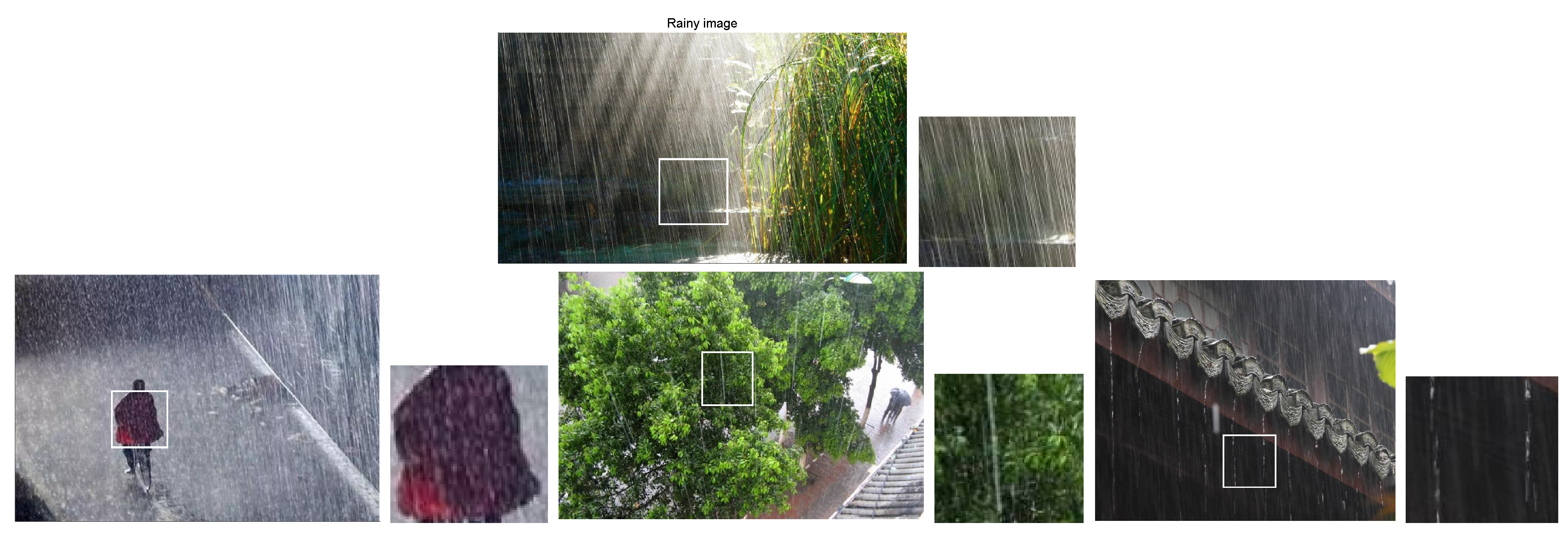
This subsection tests the performance of different methods under real rainy images. In Figure 8, the real rainy images and their local enlarged view are displayed. The testing images can be downloaded from the website.
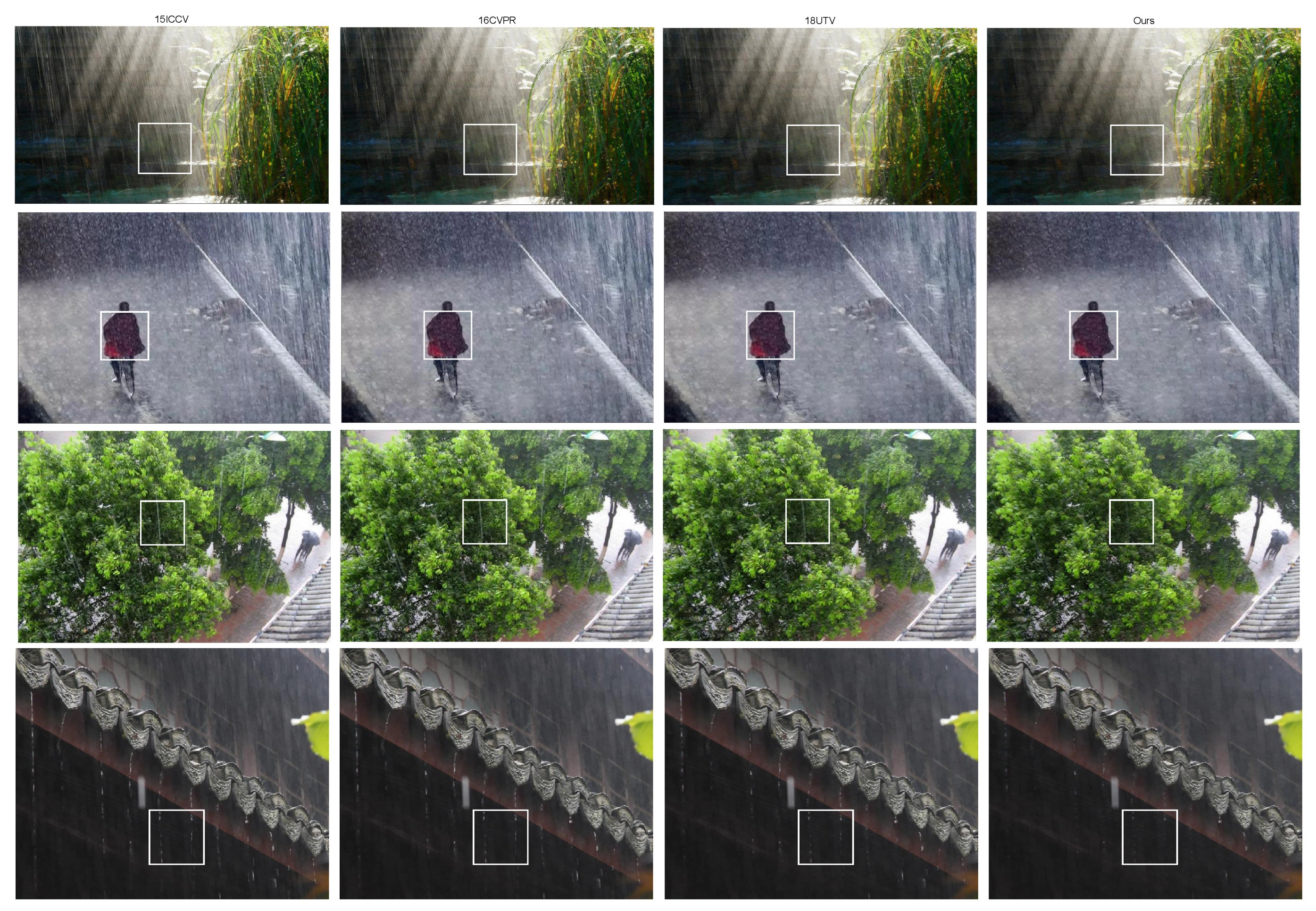
The visual results recovered by four methods are displayed in Figure 9, the first column shows de-rain results by the 15ICCV method, the second column displays the de-rain results by the 16CVPR method, the third column gives the de-rain results by the 18UTV method, and the last row shows the de-rain results by the proposed method.
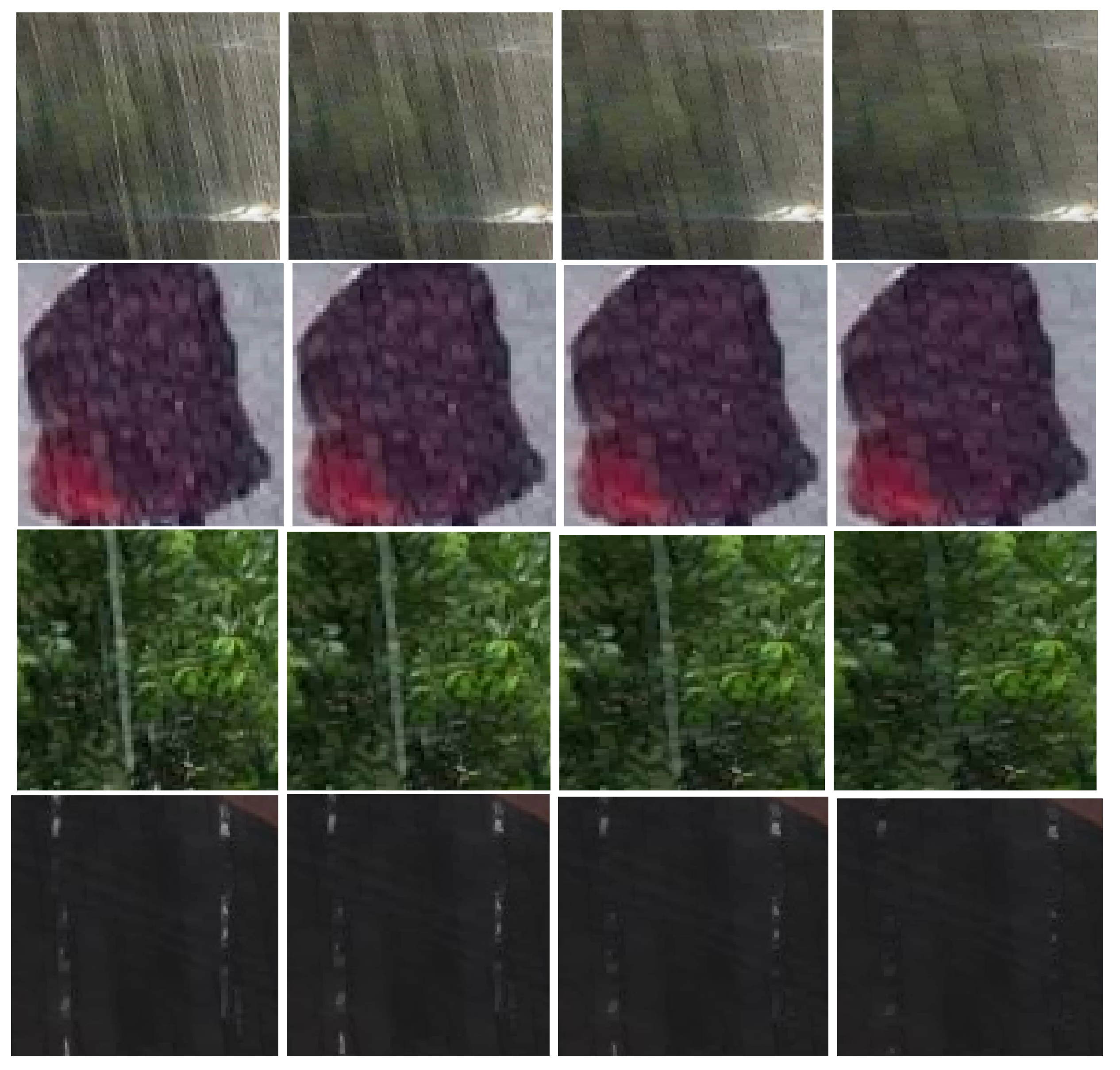
From Figure 9 and the corresponding local enlarged view in Figure 10, we can get similar results as the synthetic data. The method 15ICCV still has rain streaks remaining in the background layer, methods 16CVPR and 18UTV do significantly remove the rain streaks, but fail to detect directional singularities, while the proposed method performs well both in rain removal and detail preservation of the rain-free layer. Two test results suggest that the proposed method can remove the directional rain streaks efficiently.

6. Some Discussion for the Proposed Method

6.1. Computation Complexity

The computation complexity of our algorithm includes two Shearlets transforms computation and four sub-problems with closed-form solutions. For two Shearlets transforms, its computation complexity is about O ( N log N ) + O ( N ) . The computation complexity of four sub-problems is O ( N ) , thus the total complexity for Algorithm 1 is O ( N log N ) + O ( N ) , where N represents the total number of pixels. Table 2 shows the computation time comparison of four methods. For ’Pic1’ with size [ 559 × 314 × 3 ] , the computing time of the proposed method is 2.39 s, while the 15ICCV and 16CVPR methods take 72 s and 946 s respectively, and the 18UTV method only takes 0.87 s (without direction rotation). Our explanation is that the computation of Shearlets transform needs more computing time than UTV. Thus, we should strike a balance between the algorithm efficiency and computation complexity.

6.2. Description for Parameters

The proposed method includes two kinds of parameters, the model parameter and the algorithm parameter. For the model parameter, γ 1 , γ 2 , γ 3 are used to constrain the sparsity of Shearlets decomposition coefficients in high frequency, thus the recovery is sensitive to their changes. But different testing images with directional rain streaks are not sensitive to the parameters γ i , α i , i = 1 , 2 , 3 . In the testing, we set γ 1 = γ 2 = 1 e 3 , γ 3 = 1 e 2 , α i = 8 .
For the algorithm parameter t o l , M i t e r , they are chosen to be t o l = 1 e 3 and M i t e r = 250 . (for some images, parameters are chosen different to obtain the best result). The default setting for the 15ICCV, 16CVPR, and 18UTV methods parameters can be found in [21]. We give the average quantitative performance of 20 images of UCID in Table 3.

6.3. Simple Discussion of Regularization Terms

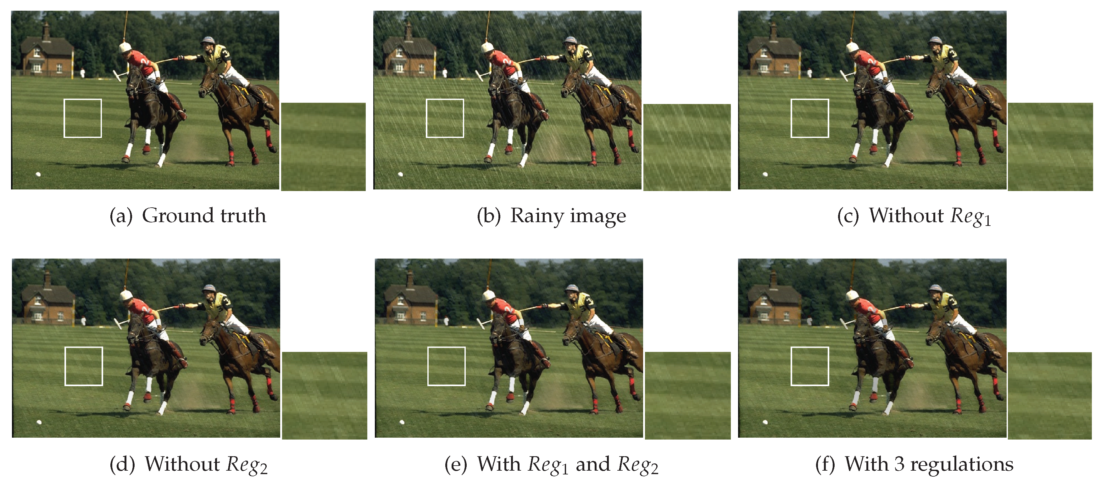
In order to understand the effect of three sparse terms, some tests are implemented to reveal their contribution for rain removal. We choose real rainy image “gentlemen” as the testing image (see Figure 11a). The visual results after discarding sparse terms R e g 1 , R e g 2 , R e g 3 are listed in Figure 11c–e. From the recovery, we find that the regularizers R e g 1 , R e g 2 have a remarkable effect on the rain removal, since R e g 1 , R e g 2 describe the sparsity of the Shearlets transform of rainy images in the rain drops’ direction and the perpendicular direction respectively.

6.4. Convergency of the Proposed Algorithm

In Figure 12, we display the convergency curve of the proposed algorithm for the testing image ‘gentleman’. It is easy to find that the RelErr value decreases as the iteration number increases, while the PSNR value and SSIM value increase with the iteration number increasing, which suggests that the proposed algorithm is stable.

7. Conclusions

This work proposed an efficient convex rain removal model for single images, which is based on the sparse prior of rainy streaks and the background layer. The split Bregman algorithm is utilized to solve our model, which ensures the global optimal. We test the synthetic and real data to demonstrate that the proposed method performs better both in rain removal and details preservation of background layer than the comparable three methods.

Author Contributions

G.S. and C.C. designed the convex optimization model for rain removal of single images and performed the experiments, G.S. and J.L. analyzed the results. G.S. wrote the paper. All authors have read and approved the final manuscript.

Funding

This research was funded by the National Natural Science Foundation of China under Grant 11271001, Grant 61370147, Grant 61573085.

Acknowledgments

The authors gratefully thank Xile Zhao for helpful discussions and the support of the National Natural Science Foundation of China.

Conflicts of Interest

The authors declare no conflict of interest.

Abbreviations

The following abbreviations are used in this manuscript:
RelRrrThe relative error
PSNRThe peak signal to noise ratio
SSIMThe structural similarity index

References

  1. Garg, K.; Nayar, S.K. Detection and removal of rain from videos. In Proceedings of the IEEE Computer Society Conference on Computer Vision and Pattern Recognition, Washington, DC, USA, 27 June–2 July 2004. [Google Scholar]
  2. Zhang, X.; Li, H.; Qi, Y.; Leow, W.K.; Ng, T.K. Rain Removal in Video by Combining Temporal and Chromatic Properties. In Proceedings of the IEEE International Conference on Multimedia and Expo, Toronto, ON, Canada, 9–12 July 2006. [Google Scholar]
  3. Barnum, P.C.; Narasimhan, S.; Kanade, T. Analysis of Rain and Snow in Frequency Space. Int. J. Comput. Vis. 2010, 86, 256. [Google Scholar] [CrossRef]
  4. Garg, K.; Nayar, S.K. When does a camera see rain? In Proceedings of the Tenth IEEE International Conference on Computer Vision, Beijing, China, 17–20 October 2005.
  5. Chen, Y.L.; Hsu, C.T. A Generalized Low-Rank Appearance Model for Spatio-temporally Correlated Rain Streaks. In Proceedings of the IEEE International Conference on Computer Vision, Sydney, Australia, 1–8 December 2013. [Google Scholar]
  6. Santhaseelan, V.; Asari, V.K. Utilizing Local Phase Information to Remove Rain from Video. Int. J. Comput. Vis. 2015, 112, 71–89. [Google Scholar] [CrossRef]
  7. Abdel-Hakim, A.E. A Novel Approach for Rain Removal from Videos Using Low-Rank Recovery. In Proceedings of the International Conference on Intelligent Systems, Warsaw, Poland, 24–26 September 2014. [Google Scholar]
  8. Tripathi, A.K.; Mukhopadhyay, S. Removal of rain from videos: a review. Signal Image Video Process. 2014, 8, 1421–1430. [Google Scholar] [CrossRef]
  9. Jin-Hwan, K.; Jae-Young, S.; Chang-Su, K. Video deraining and desnowing using temporal correlation and low-rank matrix completion. IEEE Trans. Image Process. 2015, 24, 2658–2670. [Google Scholar]
  10. Jiang, T.X.; Huang, T.Z.; Zhao, X.L.; Deng, L.J.; Wang, Y. A Novel Tensor-based Video Rain Streaks Removal Approach via Utilizing Discriminatively Intrinsic Priors. In Proceedings of the Computer Vision and Pattern Recognition, Honolulu, HI, USA, 21–26 July 2017. [Google Scholar]
  11. Yu, L.; Yong, X.; Hui, J. Removing Rain from a Single Image via Discriminative Sparse Coding. In Proceedings of the IEEE International Conference on Computer Vision, Santiago, Chile, 7–13 December 2015. [Google Scholar]
  12. He, K.; Jian, S.; Tang, X. Single Image Haze Removal Using Dark Channel Prior. In Proceedings of the IEEE Conference on Computer Vision and Pattern Recognition, Miami, FL, USA, 20–25 June 2009. [Google Scholar]
  13. Li, Y. Rain Streak Removal Using Layer Priors. In Proceedings of the Computer Vision and Pattern Recognition, Las Vegas, NV, USA, 27–30 June 2016. [Google Scholar]
  14. Kang, L.W.; Lin, C.W.; Fu, Y.H. Automatic single-image-based rain streaks removal via image decomposition. IEEE Trans. Image Process. 2012, 21, 1742–1755. [Google Scholar] [CrossRef] [PubMed]
  15. Kim, J.H.; Lee, C.; Sim, J.Y.; Kim, C.S. Single-image deraining using an adaptive nonlocal means filter. In Proceedings of the IEEE International Conference on Image Processing, Melbourne, Australia, 15–18 September 2013. [Google Scholar]
  16. Sun, S.H.; Fan, S.P.; Wang, Y.C.F. Exploiting image structural similarity for single image rain removal. In Proceedings of the IEEE International Conference on Image Processing, Québec City, QC, Canada, 27–30 September 2015. [Google Scholar]
  17. Pei, S.C.; Tsai, Y.T.; Lee, C.Y. Removing rain and snow in a single image using saturation and visibility features. In Proceedings of the IEEE International Conference on Multimedia and Expo Workshops, Chengdu, China, 14–18 July 2014. [Google Scholar]
  18. Son, C.H.; Zhang, X.P. Rain Removal via Shrinkage of Sparse Codes and Learned Rain Dictionary. In Proceedings of the IEEE International Conference on Multimedia and Expo Workshops, Seattle, WA, USA, 11–15 July 2016. [Google Scholar]
  19. Wang, Y.; Liu, S.; Chen, C.; Zeng, B. A Hierarchical Approach for Rain or Snow Removing in A Single Color Image. IEEE Trans. Image Process. 2017, 26, 3936–3950. [Google Scholar] [CrossRef] [PubMed]
  20. Zhu, L.; Fu, C.W.; Lischinski, D.; Heng, P.A. Joint Bi-Layer Optimization for Single-Image Rain Streak Removal. In Proceedings of the IEEE International Conference on Computer Vision, Venice, Italy, 22–29 October 2017. [Google Scholar]
  21. Deng, L.J.; Huang, T.Z.; Zhao, X.L.; Jiang, T.X. A directional global sparse model for single image rain removal. Appl. Math. Model. 2018, 59, 179–192. [Google Scholar] [CrossRef]
  22. Bouali, M.; Ladjal, S. Toward Optimal Destriping of MODIS Data Using a Unidirectional Variational Model. IEEE Trans. Geosci. Remote Sens. 2011, 49, 2924–2935. [Google Scholar] [CrossRef]
  23. Yang, W.; Tan, R.T.; Feng, J.; Liu, J.; Guo, Z.; Yan, S. Deep Joint Rain Detection and Removal from a Single Image. In Proceedings of the IEEE Conference on Computer Vision and Pattern Recognition, Honolulu, HI, USA, 21–26 July 2017. [Google Scholar]
  24. Fu, X.; Huang, J.; Zeng, D.; Yue, H.; Ding, X.; Paisley, J. Removing Rain from Single Images via a Deep Detail Network. In Proceedings of the IEEE Conference on Computer Vision and Pattern Recognition, Honolulu, HI, USA, 21–26 July 2017. [Google Scholar]
  25. Fu, X.; Huang, J.; Ding, X.; Liao, Y.; Paisley, J. Clearing the Skies: A Deep Network Architecture for Single-Image Rain Removal. IEEE Trans. Image Process. 2017, 26, 2944–2956. [Google Scholar] [CrossRef] [PubMed]
  26. He, Z.; Sindagi, V.; Patel, V.M. Image De-raining Using a Conditional Generative Adversarial Network. IEEE Trans. Circuits Syst. Video Technol. 2017. [Google Scholar] [CrossRef]
  27. Yin, W.; Osher, S.; Goldfarb, D.; Darbon, J. Bregman Iterative Algorithms for 1-Minimization with Applications to Compressed Sensing. Siam J. Imaging Sci. 2008, 1, 143–168. [Google Scholar] [CrossRef]
  28. Kutyniok, G.; Lim, W.Q.; Steidl, G. Shearlets: Theory and Applications. GAMM-Mitteilungen 2014, 37, 259–280. [Google Scholar] [CrossRef]
  29. Kutyniok, G. Shearlets. Appl. Numer. Harmon. Anal. 2012, 117, 14–49. [Google Scholar]
  30. Kutyniok, G.; Shahram, M.; Zhuang, X. ShearLab: A Rational Design of a Digital Parabolic Scaling Algorithm. Siam J. Imaging Sci. 2011, 5, 1291–1332. [Google Scholar] [CrossRef] [Green Version]
  31. Kutyniok, G.; Labate, D. Introduction to Shearlets. Appl. Numer. Harmonic Anal. 2012, 24, 1–38. [Google Scholar]
  32. Kutyniok, G.; Lim, W.Q. Image separation using shearlets. Preprint 2011, 1, 1–37. [Google Scholar]
  33. Zhou, W.; Alan Conrad, B.; Hamid Rahim, S.; Simoncelli, E.P. Image quality assessment: From error visibility to structural similarity. IEEE Trans. Image Process. 2004, 13, 600–612. [Google Scholar]
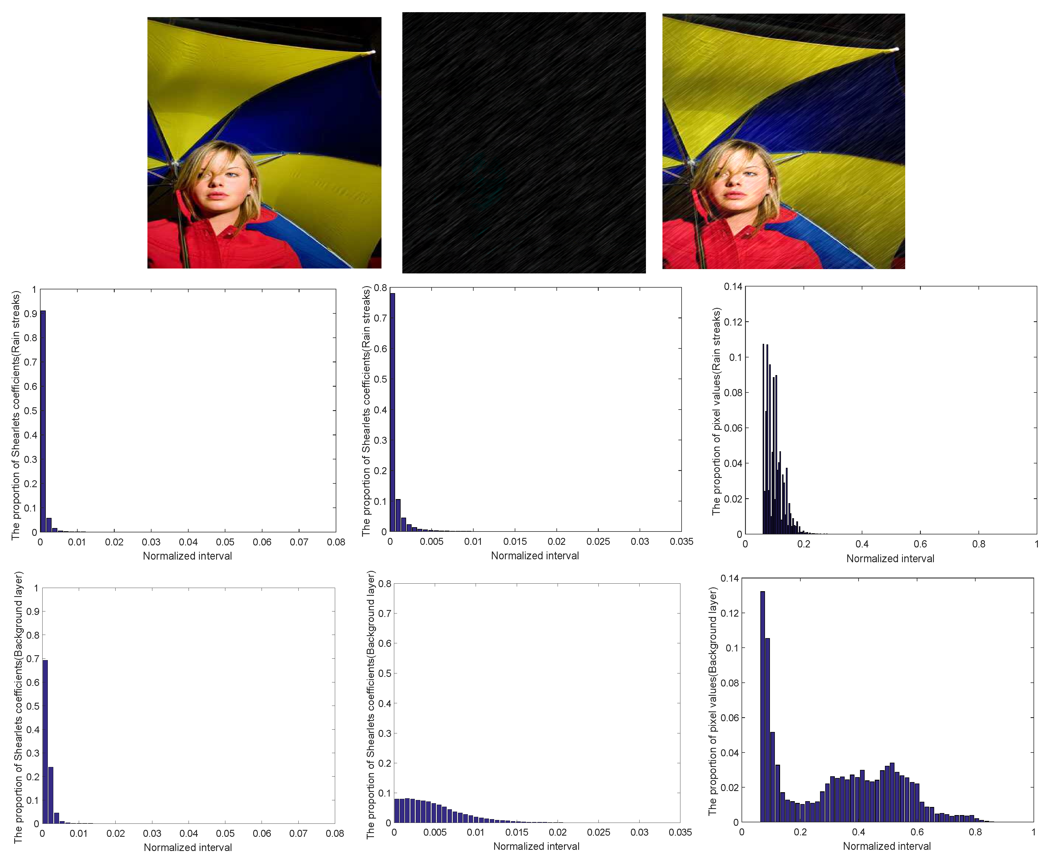
Figure 1. The sparse structure for rain streaks and the Shearlets coefficients of rain streaks and the background layer in and across the rain directions.
Applsci 09 05137 g001
Figure 2. The visual results of Shearlets decomposition coefficients in different scales (high frequency) and different directions are displayed (the testing image is “Sydney Opera House”, can be downloaded in http://homepages.lboro.ac.uk/cgs/datasets/ucid/ucid.html).
Applsci 09 05137 g002
Figure 3. The sub-band of Shearlets in the frequency domain.
Applsci 09 05137 g003
Figure 4. The ground truth and rainy image of synthetic testing images.
Applsci 09 05137 g004
Figure 5. The visual results of four methods for synthetic images.
Applsci 09 05137 g005
Figure 6. The corresponding local enlarged view of four methods for synthetic images.
Applsci 09 05137 g006
Figure 7. Relative error (RelErr), peak signal to noise ratio (PSNR), structural similarity index (SSIM) performances on 20 images.
Applsci 09 05137 g007
Figure 8. The real rainy images.
Applsci 09 05137 g008
Figure 9. The visual results of four methods for real rainy images.
Applsci 09 05137 g009
Figure 10. The corresponding local enlarged view of four methods for real rainy images.
Applsci 09 05137 g010
Figure 11. Recovery without different regularizer terms.
Applsci 09 05137 g011
Figure 12. The variation of RelErr, PSNR, SSIM values with the iteration number.
Applsci 09 05137 g012
Table 1. The parameters list.
Parameters den len θ °
1[0.02, 0.04, 0.06, 0.08]1030
20.04[10, 20, 30, 40]15
30.0410[−15, −5, 0, 5, 15]
Table 2. Results comparison on synthetic data.
Rainy TypeHeavyLight
BackgroundRainy StreaksTimes(s)BackgroundRainy StreaksTimes(s)
ImageMethodsPSNRSSIMRelErrPSNRSSIMRelErr PSNRSSIMRelErrPSNRSSIMRelErr
Pic115ICCV28.790.867311.83227.510.483115.64271.5429.840.900210.27327.160.49511.41678.32
16CVPR30.490.88927.68230.670.64177.394948.2730.760.912310.79130.520.53310.376941.96
18UTV30.830.90277.59130.910.67937.4270.8732.870.93455.96432.790.64975.8730.68
Ours31.620.91158.24430.760.69547.0822.3933.280.94525.41733.190.67195.3142.26
Pic215ICCV27.120.811712.02727.010.419312.31473.9428.960.893610.21728.740.401910.12782.37
16CVPR28.540.86299.26428.310.576310.028926.8529.940.91879.02629.780.469310.201931.57
18UTV30.170.90568.314630.090.64938.2170.9432.690.92217.42431.790.60197.6190.79
Ours31.680.91958.02730.590.69528.3354.0832.940.92077.50632.840.63946.7013.15
Pic315ICCV27.640.832710.83727.280.423710.31698.6930.960.90177.46229.850.51737.43896.54
16CVPR28.940.87258.49729.030.48879.287837.2932.150.91027.417932.360.57827.419864.61
18UTV30.420.90137.69430.250.54737.4151.2932.830.92747.01832.590.59956.1311.25
Ours31.520.91138.91730.830.5917.49534.7633.650.94316.29433.460.65545.8314.93
Pic415ICCV26.840.791613.9426.950.401714.9280.6429.070.81149.14828.960.477110.16782.17
16CVPR28.410.879211.6428.440.465710.131147.0932.180.91048.36532.060.49939.7251129.68
18UTV32.170.92088.6132.070.61298.4861.1732.360.95027.62831.590.61078.8471.89
Ours31.880.91598.0532.160.62837.9713.8732.870.92217.39132.720.61947.8723.84
Pic515ICCV29.760.833910.01730.010.49969.17244.9332.690.90177.28632.540.51627.83631.26
16CVPR31.940.89928.27431.790.51947.139428.1633.940.93176.26433.720.59976.938441.27
18UTV33.260.93316.19233.860.59176.9850.6134.920.94275.94734.940.6275.8460.57
Ours31.860.91417.21430.940.57118.7182.9532.090.91977.17230.520.68449.8733.17
Table 3. Average quantitative performance of 20 images from UCID with different types of rain streaks.
Rain TypeMethodsBackgroundRainy StreaksTime(s)
PSNRSSIMRMSEPSNRSSIMRMSE
d e n = 0.04 15ICCV28.74 ± 2.490.8293 ± 0.051311.57 6 ± 2.89526.19 ± 3.420.4702 ± 0.052713.042 ± 3.521144.27
l e n = 40 16CVPR29.64 ± 2.010.8846 ± 0.03129.142 ± 1.25927.41 ± 1.390.5327 ± 0.09329.741 ± 1.6921152.64
t h e t a = 0 18UTV30.74 ± 0.630.8811 ± 0.07379.747 ± 0.99427.94 ± 0.530.6017 ± 0.05749.226 ± 1.7261.59
Ours31.02 ± 1.7220.8842 ± 0.03978.117 ± 0.69228.52 ± 0.630.6064 ± 0.08278.017 ± 0.9233.94
d e n = 0.08 15ICCV26.39 ± 1.640.7923 ± 0.624912.971 ± 2.06327.73 ± 1.360.4713 ± 0.053912.973 ± 2.918119.57
l e n = 40 16CVPR28.94 ± 1.920.8709 ± 0.031910.559 ± 1.94728.59 ± 2.740.5904 ± 0.17529.172 ± 2.0721397.46
t h e t a = 15 18UTV29.59 ± 2.170.8906 ± 0.02169.311 ± 1.50928.74 ± 1.9150.6607 ± 0.079310.703 ± 1.4481.97
Ours30.16 ± 1.430.9042 ± 0.01619.942 ± 1.77228.94 ± 2.730.692 ± 0.11549.954 ± 2.1424.57
d e n = 0.04 15ICCV28.74 ± 1.890.8841 ± 0.071911.409 ± 1.17328.97 ± 1.830.5516 ± 0.096712.712 ± 1.83786.53
l e n = 40 16CVPR30.55 ± 1.930.892 ± 0.051710.929 ± 1.84630.59 ± 1.730.6012 ± 0.095310.397 ± 2.0661493.27
t h e t a = 15 18UTV31.27 ± 1.530.9004 ± 0.04397.492 ± 0.79331.37 ± 1.740.6112 ± 0.057110.973 ± 0.7221.38
Ours31.42 ± 1.710.9087 ± 0.01647.928 ± 0.27132.17 ± 0.540.6292 ± 0.08039.364 ± 0.5744.61