Article

Short CFD Simulation Activities in the Context of Fluid-Mechanical Learning in a Multidisciplinary Student Body

by
Manuel Rodríguez-Martín
1,*,
Pablo Rodríguez-Gonzálvez
2,
Alberto Sánchez-Patrocinio
1 and
Javier Ramón Sánchez
3
1
Department of Mechanical Engineering, Universidad de Salamanca, 37008 Salamanca, Spain
2
Department of Mining Technology, Topography and Structures, Universidad de León, 24071 León, Spain
3
Department of Chemical and Textile Engineering, Universidad de Salamanca, 37008 Salamanca, Spain
*
Author to whom correspondence should be addressed.
Appl. Sci. 2019, 9(22), 4809; https://doi.org/10.3390/app9224809
Submission received: 29 October 2019 / Accepted: 8 November 2019 / Published: 10 November 2019

Abstract

:

Featured Application

Improved training of engineers in the industrial branch and instruction of students in fluid simulation tools.

Abstract

Simulation activities are a useful tool to improve competence in industrial engineering bachelors. Specifically, fluid simulation allows students to acquire important skills to strengthen their theoretical knowledge and improve their future professional career. However, these tools usually require long training times and they are usually not available in the subjects of B.Sc. degrees. In this article, a new methodology based on short lessons is raised and evaluated in the fluid-mechanical subject for students enrolled in three different bachelor degree groups: B.Sc. in Mechanical Engineering, B.Sc. in Electrical Engineering and B.Sc. in Electronic and Automatic Engineering. Statistical results show a good acceptance in terms of usability, learning, motivation, thinking over, satisfaction and scalability. Additionally, a machine-learning based approach was applied to find group peculiarities and differences among them in order to identify the need for further personalization of the learning activity.

1. Introduction

Computational strategies such as Computational Fluid Dynamic (CFD) are usually applied to simulate fluids (gas and liquids) to obtain different physical variables such as pressure, velocity, mass rate, turbulence energy, temperature, turbulence intensity, vorticity, and others. Based-on CFD applications work over a computational domain using partial differential equations (PDE) and ordinary differential equations (ODE) to describe the relationship among different physical variables to understand the characteristics of fluid flow. The specific applications of the method can be very diverse, depending on the objectives of the analysis, the required accuracy and other factors, such as computing times (which can be high, namely, from hours to days) [1]. The main applications of CFD encompass aerodynamic analyses, multi-phase flows, transport, compressible flows, phenomena and chemical processes involving transfer heat phenomenon, dissipative phenomenon, rotary, mixing of different fluids and chemical reactions [1,2,3,4,5].
Furthermore, specific CFD software can be difficult to handle and, sometimes, unintuitive for students without previous experience. Carrying out processing tasks using CFD can become a long, hard and intense work when it is performed for specific applications [1], for example, optimization [3,6], model calibration [7], sensitivity analysis and consequence analysis [8]).
As it is established in [9], within the CFD context, the Finite Volume Method (FVM) is a specific numerical iterative technique that involves partial differential equations (mainly representing conservation laws) applied over differential volumes. This discretization process is similar to the Finite Element Method (FEM) [9]. The meshing procedure is highly important in the FVM method because it strongly affects the accuracy and stability of the flow predictions [10]. The meshing consists of the generation of a grid over the fluid computational domain. This grid can be generated for the computational model with different typologies (mainly structured, non-structured and hybrid) being a quality mesh essential for a quality simulation [11]. Through the mesh, the discretization of the volume is obtained and the partial differential equations are discretized into algebraic equations by integrating them over each discrete volume element. As a result, a discrete number of algebraic equations are established over a finite number of volumes from application of the meshing process to the whole study volume. These algebraic equations are solved as an algebraic equation system to calculate and compute the values of the dependent variable of each discrete volume element. An adequate mesh design is critical, since the accuracy of the results of the simulation process highly depends on how well the equation system or the mathematical model captures the flow physics [1].

1.1. CFD Method in the Learning Context

The CFD method has been used as a teaching resource for university studies, specifically, for undergraduate courses in engineering [12,13,14]. Nevertheless, simulation methods such as CFD and FEM are frequently offered as specific elective course in many academic institutions around the world for the acquisition of competence in simulation [1]. However, the assimilation of the learning of these types of tools involves long training times and it could be an impediment in the context of basic courses in engineering programs, considering the usual intensity of the scholarship for students and professors [15]. In this way, specific strategies can be used to integrate CFD in basic courses in engineering, specifically in the fluid-mechanics course [15].
The calculation of energy losses in pipes is an important skill which students must achieve in the fluid-mechanical course. Pressure drop in a pipe system is caused by fluid rising in elevation, shaft work, friction, and turbulence from sudden changes in direction or cross-sectional area [16]. Specifically, the calculation and application of pressure loss coefficients for different pipe sizes is important to calculate the energy loss and pressure drop in pipes and specific hydraulic elements installed in the line and, in this way, determine important parameters for engineering tasks, such as determining the correct pump size [17]. A summary of the published literature about pipes fitting in the learning context is established in [1]. When the pipe has a complex internal geometry or specific elements are installed in the pipelines (nozzles, valves, elbows, filters, etc.), the energy losses can be obtained experimentally or through simulation tools such as CFD. However, pressure drop in singular elements can be also calculated using empirical tables and/or graphics, available in the literature (e.g., [11]). Unfortunately, the casuistry of this method based on the literature is reduced for several reasons: Limited number of head loss elements and also limited since ideal conditions are considered as ideal geometries for the elements, single-phase flow, Newtonian fluids, no consideration of the material type of the solids, etc. [15]. However, fluid-mechanical industry problems are sometimes more complex, including multiple phases, complex boundary conditions and complex geometry of the volume. These problems cannot be addressed using only the classic equations and empirical tables and/or graphics; nevertheless, they can be addressed using computer methods based on CFD. Thus, it is important that students, as future professionals, understand the scope and significance of this issue and the limitations of theoretical methods explained in the classroom [15].
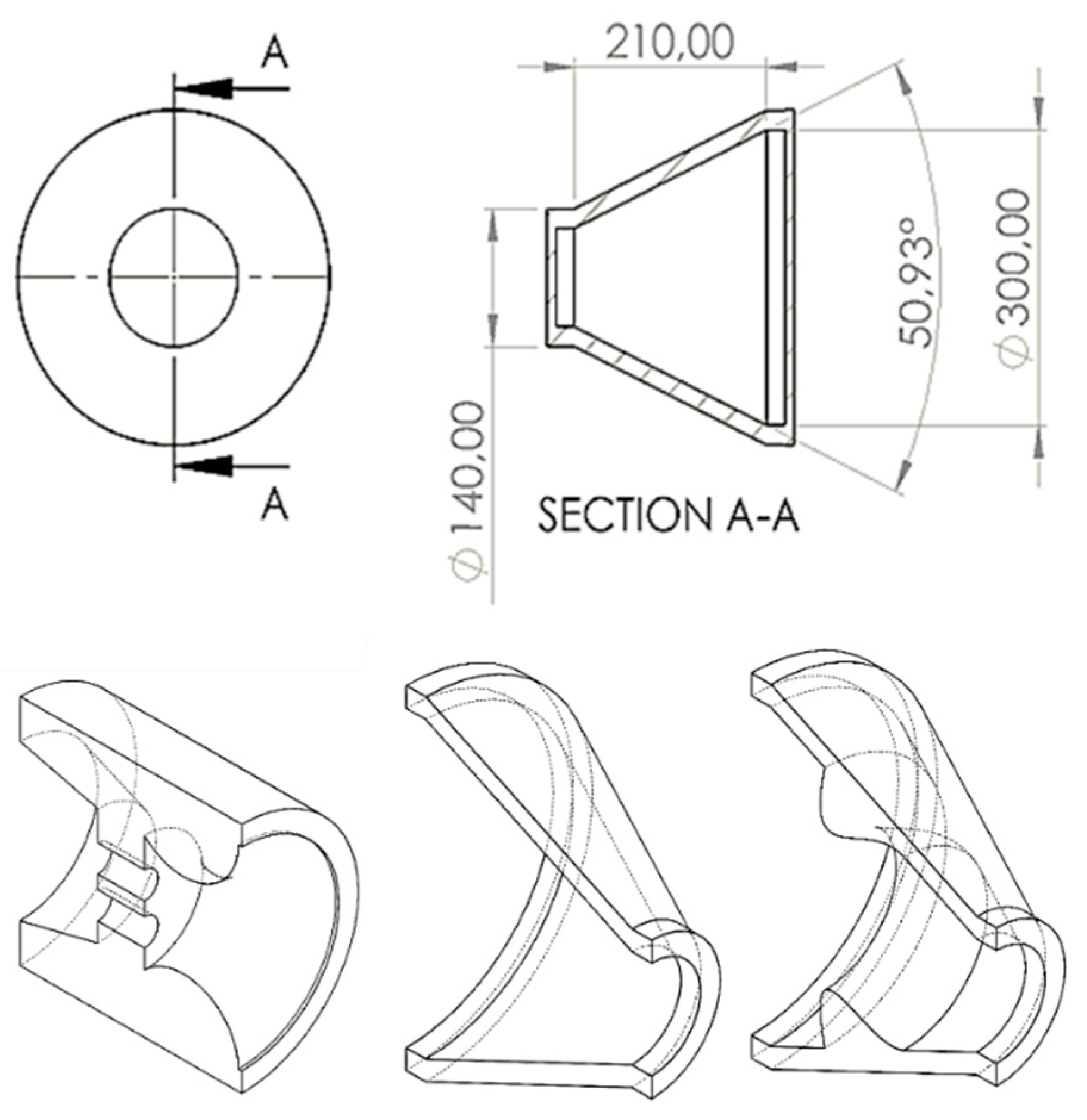
Students tend to identify pressure drop with the concept of pressure drop “in line” (caused by friction with respect to the pipe). However, pressure drop is a wider concept which includes the local pressure loss caused by specific elements located in the fluid line, such as contractions or expansions, valves, etc. Due to this simplification of a complex reality, students sometimes ignore the fact that pressure drop can be caused by apparently insignificant anomalies in the geometry of the pipeline.
Teaching this concept in a laboratory using experimental equipment is often expensive because some sophisticated stations and instruments are required [1]. Taking into account the high economic cost of the specific instrumentation, the amount of time spent doing the experimental tasks with the students, and operational limitations (e.g., presence of large groups of students) justifies the creation of virtual laboratory resources to support teaching activities [18]. These initiatives share many objectives with respect to simulation activities, insofar as they replace or complement experimental laboratory lessons. Besides, CFD could be an adequate tool to explain concepts that complement the theoretical classes to understand the pressure drop phenomenon, while we are providing the student with very useful software skills which can be important for their future professional career. The fluid-mechanical course is a subject common to all engineering degrees in the industrial teaching program, but, as has been mentioned, learning times for the CFD method of the tool are normally long. Concurrently, machine-learning based methodologies have shown great potential for pattern recognition and predicting results for multiple types of datasets, in spite of the field using supervised algorithms for most of these works. The results of these methods can be incorporated into the decision-making process [19], even for strategic decision making at higher educational institutions [20], predicting the performance of the students in blended learning [21] or prediction of early dropout [22].

1.2. Research Question

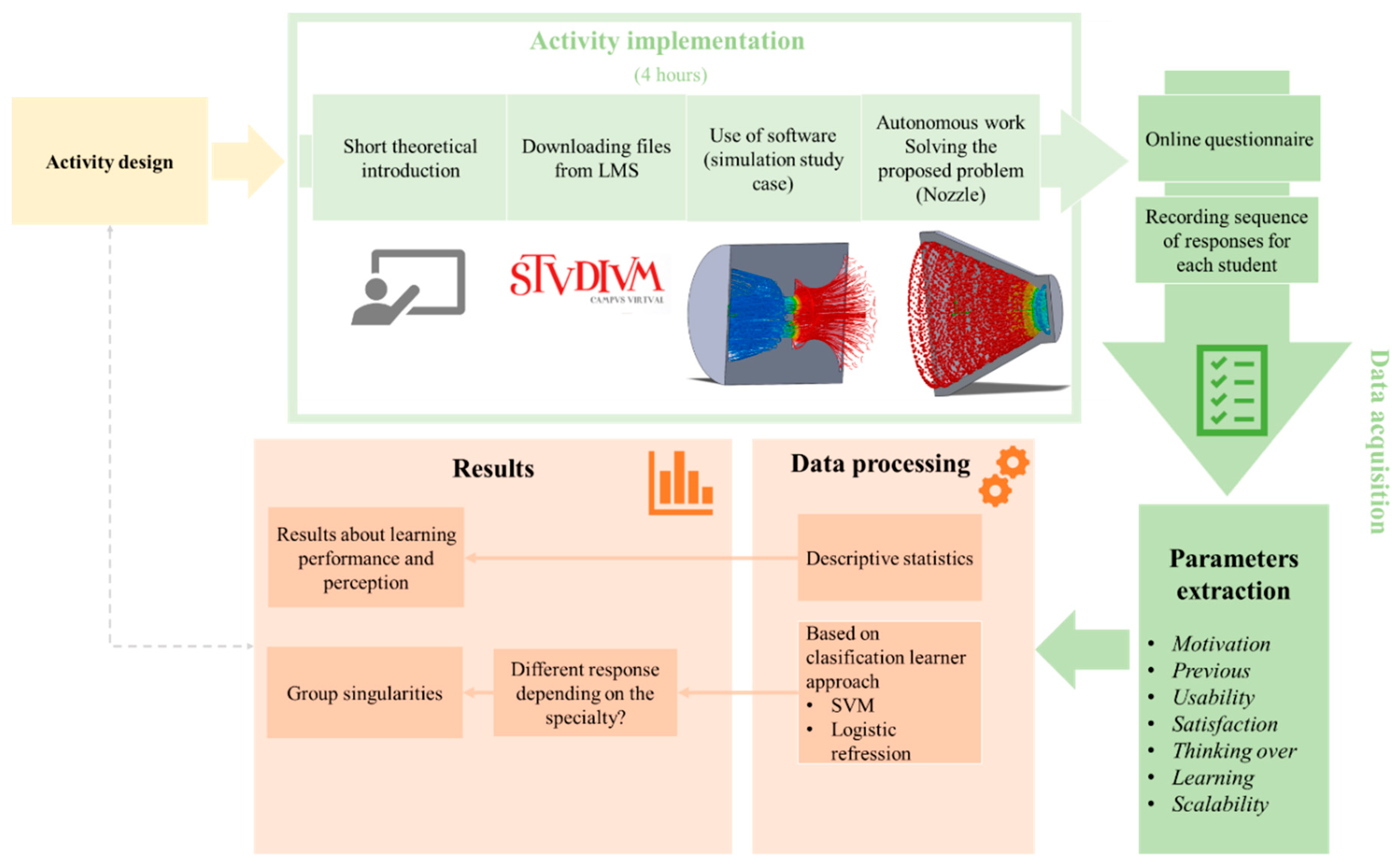
The research question can be divided in two parts: First, we want to know if the specific use of short practical activities using the CFD module of Solidworks® [
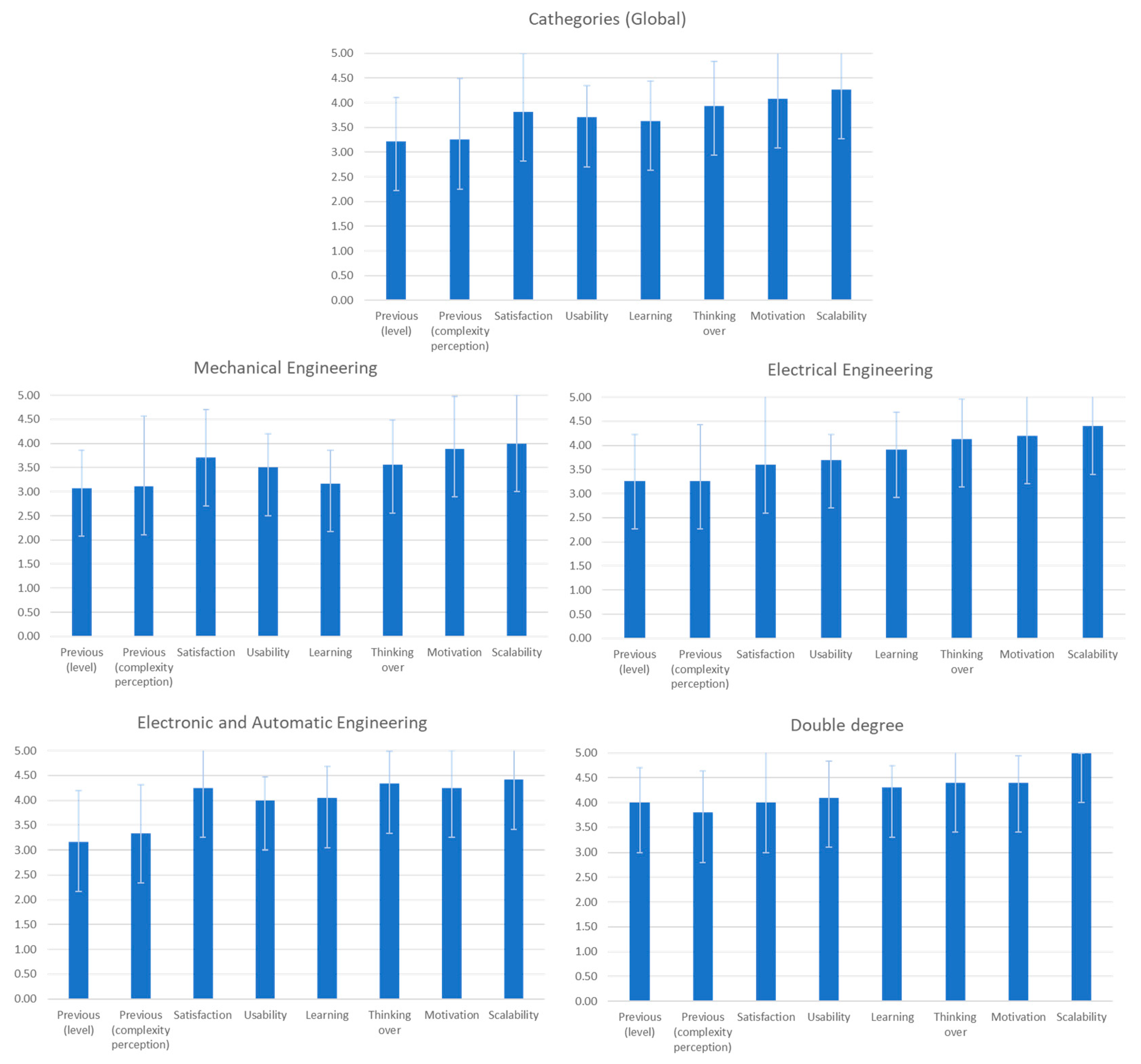
23] is appropriate for the goals raised. Mainly, we want to know whether its use is adequate in terms of usability, satisfaction scalability, learning, thinking over and motivation, which are the most analyzed issues in education [24,25,26]. Please note that we study the activity’s motivation since it is linked with academic performance [27]).
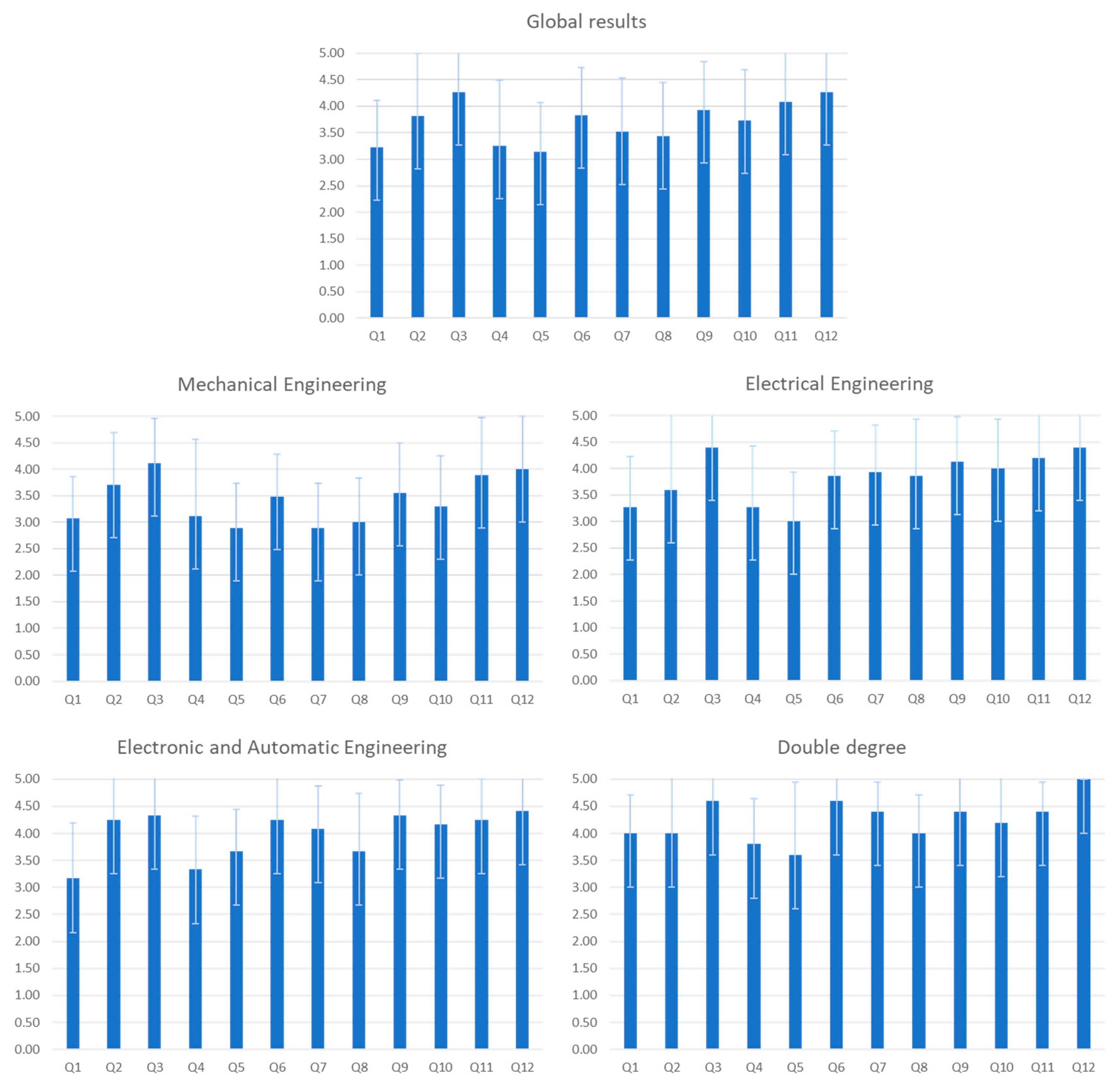
Secondly, by means of a machine-learning approach, we want to know whether the response to the activity is independent of the bachelor’s degree of origin or, on the contrary, there are questionnaire response patterns. The presence of a pattern that differentiates the activity’s response depending on the bachelor degree will justify future modification to adapt the learning activity.

2. Academic Context of the Research and Sample

This research was implemented in the fluid-mechanical subject. This subject is established as mandatory in the second year for the following three bachelor degrees: Mechanical Engineering, Electrical Engineering and Electronical and Automatic Engineering, at the Higher Technical School of Industrial Engineering of Béjar of the University of Salamanca (Spain).
The specific competences (Table 1) of the subject are based on the Spanish regulation [28] which derives from the regulations of the European Higher Education Area (EHEA). The three degrees belong to the industrial engineering field (Figure 1), so the first two courses are common for the three bachelor’s degrees while the last two courses are considered as specialization courses and they are different for each one. Some colleges offer double degrees. In this case, students enrolled in the double degree in Electrical and Mechanical Engineering are contemplated in the sample. According to Spanish regulations for the engineers, some engineering tasks can be done indistinctly by any of the engineers of the industrial field, while other more specialized tasks can be done specifically by only one of them (e.g., under Spanish regulation, electrical low voltage projects can be carried out by any industrial engineer, but high voltage projects can only be carried out by electrical engineers). Please note that the B.Sc. in Chemical Engineering is not offered by the High School of Industrial Engineering of the University of Salamanca, so it was not analyzed in the present work.
The research was addressed over a sample of 59 students of the fluid-mechanical subject. In spite of the fact that the students came from different grades, they were grouped together in the same classroom since it is a common subject. The distribution of the sample is shown in Table 2.

3. Materials and Methods

3.1. Materials

In [15], a previous requirement and potentialities study about the learning activity was raised. As a result, Solidworks® [23] was chosen as teaching software. It is a CAD/CAM/CAE commercial package software with extensive functionalities within the context of mechanical engineering. In summary, this software was chosen for three reasons: (i) Ease of use of the CFD module compared to other CFD software alternatives. The simplicity of use was established as a critical factor to reduce the time assigned for the activity (please note that one of the factors which will be evaluated is the usability); (ii) the object’s geometry can be modeled using the same software in an easy way without the need to use other applications, saving time; (iii) the software can be used in other subjects and by other professors in their teaching. Solidworks® was installed in one of the computer classrooms of the Higher Technical School of Industrial Engineering, which is equipped with individual work station posts.
Additionally, to distribute the different activity materials to the students, the documents and files were uploaded to the institutional Learning Management System (LMS) of the University of Salamanca (Studium).

3.2. Methods

A specific methodology to evaluate the performance of the activity in different terms was raised for this research in an ad hoc manner (Figure 2). The different phases of the methodology will be described in the following paragraphs.

3.1.1. Activity Design and Completion

The learning activity was designed through a deep reflection under three important criteria, which were established as a reference for the creation of the learning resources and virtual models for the activity: Quality, economy and reality criteria [15]. These were established in the literature for the virtual environments [18,29,30] and, as has been previously indicated, the authors consider that simulation tasks share objectives and needs with respect to virtual laboratories: The common mission to provide to the student a practical vision about the physical phenomena without using, or complementing, a real laboratory for experimental tasks. According to the reality criterion, the activity is intended to be clear enough to simulate a real behavior of the fluid with adequate visualization results, based on the study of trajectories or particles, as well as maps of the distribution of different variables. The economy criterion refers to the balance between available resources and needs. In this respect, it is required for the simulation process to be as short as possible, so there is no wasted time in computation tasks. This is due to the high concentration of activities that must be completed in the subject and the fact that the simulation process has to be carried out entirely using the available workstations, without acquiring new ones. Toward this goal, various preliminary tests were carried out by the authors to find the simulation case that balanced processing times and results accuracy and met these conditions without affecting the other criteria. The processing times obtained for an adequate accuracy were between 180 and 350 s. Finally, the quality criterion implies that the results have an acceptable accuracy for learning tasks, and all the resources and documents necessary for the activity and for its evaluation can be distributed in LMS (please note that the upload file size limitation is a considered constraint parameter for the activity design).
Due to the proposed reflection, the activity was designed in four phases. Students were divided into two heterogeneous groups in order to achieve a better teacher-student ratio. The same activity was carried out with each of the groups in consecutive weeks. The first three phases (Figure 2) were oriented to the explanation of the activity and the basic concepts: Firstly, a short theoretical lesson about the CFD method was explained; next, students downloaded from the LMS the archives and documents for the activity; and finally, a simulation of an irregular conduit (Figure 3) was presented by the professor while the students were following the steps at the same time.
The fourth phase (Figure 2) was oriented to the autonomous work of the student (practical case), which consisted of the simulation of two hydraulic nozzle models: Smooth and obstructed ones. The obstructed hydraulic nozzle model was designed with respect to the smooth one to compare the obtained results for the two simulations and to compare those with the theoretical results obtained with the Bernoulli equation.
A hydraulic nozzle is really a single hydraulic device used to increment the velocity of the incompressible fluid through a reduction of the effective section. When the nozzle is smooth and clean, the fluid flows in the usual way, following a behavior close to the Bernoulli equation, which is established under ideal flow conditions in the absence of dissipative phenomena. Nevertheless, if the nozzle has an obstructed zone, a significant pressure drop is generated and, in this way, the velocity, pressure, turbulence and other parameters of the fluid differ from the results obtained using the Bernoulli equation for the same initial parameters. Therefore, this situation allows the students to think about the limitations of theoretical methods with respect to experimental methods. Please note that the design of the obstructed nozzle model does not respond to a real case but is an example that has been generated so that the simulation activity would meet the criteria indicated above. The parameters for the simulation indicated to the students in the problem statement are shown in Table 3 and all of them have been established to accomplish the established criteria for the creation of learning resources.
The activity was implemented in the classroom following the established plan for four hours, of which 200 min were used in the students’ autonomous work. Two professors were present during the activity, observing the behavior of the students and resolving any doubts they may have. The professor–student rate was 15 students per professor.

3.1.2. Data Gathering

Once the activity was implemented in the classroom, the data gathering process was carried out to obtain the results to evaluate the suitability and acceptation of the learning activity. An anonymous online questionnaire, which can be fulfilled in 5 min, was designed. The questions are shown in Table 4. The response type is yes/no for the three first questions and for the rest a Likert scale is used [18,29,30]. For the analysis, each question was grouped into one of the categories described in Table 5. The complete pattern of responses for each student was obtained anonymously.

3.1.3. Descriptive Statistical Analysis

The instrumentation applied was an online short questionnaire (Table 4) with two response types: A yes/no answer and a Likert scale. Twelve of the fifteen items of the questionnaire were designed based on a 5-point Likert scale [31]. All answers were raised in terms of the level of agreement (1-Strongly disagree, 2-Disagree, 3-Neither agree or disagree, 4-Agree, and 5-Strongly agree). The scale was chosen to seek simplicity and homogeneity in the answers so as not to generate erroneous or confused answers while making an accurate interpretation of the data.
The results for each question whose response is yes/no was statistically computed using the frequency of each response. The results for each question that used the Likert scale were statistically analyzed through the mean and standard deviation values. Parametric statistics were chosen as they are sufficiently robust to yield correct results when Likert scale answers are analyzed [32]. The same process was applied for the results obtained for the different categories: Average of the questions’ answers for each category. For this analysis, the response of each student for each question was analyzed individually by means of a classic statistical approach; therefore, questionnaire response patterns are not taken into account in the descriptive analysis.

3.1.4. Based on ML Approach to Detect Group Characteristics

Once the descriptive analysis was addressed, differences of the mean values for each question among the different groups were identified. A machine-learning classification strategy was implemented to corroborate if there were differences between the responses to the activity for each group (Table 3). For this, the individual questionnaire response pattern of each student was included in the analysis.
The results obtained for each student are classified in function of the B.Sc. degree (mechanical, electrical and electronic, and automatic engineering) in order to analyze if the machine-learning classifier would be able to detect a significant pattern that allows us to classify each student to their degree in function of the questionnaire responses. The set of students’ responses for each bachelor degree will be two-to-two compared using four different classification learners. These methods have been chosen based on the literature for similar cases [33] and also considering the adequacy of success indicators: Support machine vectors (SVM), logistic regression (habitually used in social sciences), random forest, and Bayesian network.
Firstly, SVMs are algorithms built on the theory of statistical learning aimed at minimizing structural risk. In pattern recognition, classification and regression analysis, it is expected that SVMs outperform other machine-learning methodologies [34]. An SVM is a discriminative classifier that looks for the optimal hyper plane that categorizes the training data. Secondly, the classifier based on logistic regression identifies specific parameters of the logistic function linked features with respect to binary target variables [33]. Its prediction function (logistic/sigmoid function) depicts the curvilinear relationship between the inputs and outputs. Therefore, the output’s coefficients provide the relationship between a binary variable and several independent variables. Thirdly, random forest is an ensemble classifier that produces many classification and regression-like trees where each tree is generated from different bootstrapped samples of training data [35]. Random forest enables many weak or weakly-correlated classifiers to form a strong classifier [36]. Finally, the Bayesian network is one of the most effective classifiers [37] and is very useful tool to define logical relationships among variables in complex models. It is a probabilistic graphical model that expresses the relationships among a set of variables that quantify the links between variables based on their conditional probabilistic relationship [38].
For the machine learning analysis, the open software Weka [39] was used. Different training experiments were implemented in order to choose the most adequate prediction features and the optimum machine learning parameters. For the assessment of the classification k-fold cross-validation was employed, which splits the training data into k equal-sized partitions [40]. If the applied machine learning algorithm can classify successfully, this implies that there is a questionnaire response pattern for each group (mechanical, electrical or electronic engineering). Namely, it will be possible to predict the student’s degree as a function of the different measured characteristics.
The machine learning classification results are evaluated in terms of the overall accuracy, the Cohen’s Kappa index and the receiving operating characteristic (ROC) curve area. The Kappa statistic measures the degree of agreement of categorized data [41]. It is defined in the range of −1–1, with zero being the expected value for a random classification, 1 being a perfect agreement, and negative values indicating no agreement, although they are unlikely in practice. The area under the ROC curve (AUC) provides a comparison between the predicted and actual instance values in a classification by measuring the precision and the recall [42]. It measures the probability that randomly chosen instances will be correctly classified. It is widely used for model comparison, since it describes the model performance for a complete range of classification thresholds. The ROC area is defined in the range 0–1, with 0.5 being the expected value for a random classification. Therefore, AUC values equal to or less than 0.5 imply that the classifier has an efficiency that is not superior to randomness, not being effective in this case.

4. Results

4.1. Descriptive Analysis

As the reader can see in Table 6, the 54.2% of students have worked previously using a parametric design application as Solidworks® or similar CAD tools, but only 10.2% of students had used a CFD method before. This means that for the majority of the sample, it is the first time that they used this technology, which excludes biases due to possible previous experiences. Considering the results of the previous answer, approximately half of students have used CAD/CAM/CAE tools for 3D design, but not for fluid simulation, although 91.5% of the students knew about the existence of CFD applications.
The statistical results (mean and standard deviation) for each question are shown in Figure 4 and Table 7. It can be seen that the main values for all of the questions are above 3 out of 5, while the standard deviation values shows a low dispersion with respect to the mean value (close to 1 in all cases). This assessment is supported by the Z-test of the 66 possible combinations for the 12 questions, with a p-value always higher than 0.05 (95% confidence). Namely, there is no significant difference among all answers.
Additionally, the analysis will be carried out from the characteristics extracted from each question (Table 4). In this manner, eight important characteristics are extracted from the results of the questions for each student. Mean and standard deviation of the distribution are show in Figure 5 and Table 8. All the results for the eight characteristics have a mean value above the 3 over 5. In global terms, it points outs a good acceptance of the activity in all the measured aspects. Furthermore, the standard deviation is also close to 1 for each case, which indicates that the dispersion tend in the responses are low. Motivation and scalability are the results which higher mean values while the usability result is slightly lower than the rest. This last issue was predictable due to the usual difficulty to handle CFD software; even though the software chosen for the learning activity has an easy handling compared to other CFD alternative applications.
When the results are analyzed by groups (from each B.Sc. degree) the reader can observe both differences and trends in the results. For all the groups, the scalability is the characteristic that achieves the greatest mean value (greater than 4 for all the groups). The second characteristic which greater results obtain is the motivation for Mechanical Eng., Electrical Eng. and double degree but for Electronic and Automatic Eng., the second place is for the thinking over. However, the mean values for Mechanical are slightly lower than the rest, especially in learning (3.17).

4.2. Machine Learning Classification Approach

The machine learning approach aims to analyze whether the answers provided by the students are conditioned or not by their particular degree. The comparison is carried out for each two degrees as shown in Figure 6. If the classifier provided an adequate classification on the basis of success indicators (precision, overall accuracy, Kappa index and AUC), there is an effective different response pattern for each of the degrees.
Machine learning algorithms are trained using different variables to obtain the best results using the prediction features stated in Table 9, which showed better indicators of success. The most effective parameter to evaluate the prediction capacity of each method is the AUC. If this value is 0.5 or less, the algorithm is making predictions with an accuracy close to randomness. It means that a classification is not possible for the algorithm.
As is shown in Table 10, based on features applied (Table 9), the AUC is above 0.5 for the comparison between the B.Sc. degrees in electrical engineering and the B.Sc. degree in mechanical engineering. For the comparison between the B.Sc. degree in electronic and automatic engineering with respect to the B.Sc. degree in mechanical engineering.
However, for the comparison between the B.Sc. degree in electrical engineering with respect to the B.Sc. degree in electronic and automatic engineering. Therefore, the classifier could not predict successfully (lowest values for the four indicators of Table 9).
Please note that the data collection is limited, and very different subjective parameters are being evaluated, so the AUC and Kappa values do not show the high accuracy typical of other applications of machine learning [43,44]. However, this analysis is not oriented to establish a high accuracy predictive algorithm, but this approach is oriented to demonstrate differences in the questionnaire response patterns for each student. If it is possible to predict the degree, then it is demonstrated that degree conditioning factors to the activity in a non-homogeneous sample with students from different B.Sc. degrees who carried out the same activity at the same time. Different experiments were carried out in order to find the predictor features which provide better Kappa and AUC results.
When the questionnaire answers are compared between the B.Sc. degrees in electrical engineering and the B.Sc. degree in mechanical engineering, the best results are obtained with the Bayesian network classifier, achieving an overall accuracy of 80.9% and a Kappa index of 0.530. These results are significant for the quality of the success of the classification between the two groups. Regarding the AUC, for all four tested classifiers the value obtained is higher than 0.5, being the most optimal AUC result (0.768) obtained for the random forest classifier.
In the comparison between the B.Sc. degrees in mechanical engineering and the B.Sc. degree in electronic and automatic engineering, the Bayesian network classifier achieved the best results, with an overall accuracy of 84.6%, a Kappa index of 0.581 and an AUC of 0.728. The rest of the classifiers achieve lower performance results, but always higher than the randomness threshold (0 for Kappa, and 0.5 for AUC).
While for the two comparisons mentioned above the algorithm test can classify with acceptable accuracy the response patterns (results parameters with a success rate higher than randomness), when the same classifier algorithms are trained and applied between the B.Sc. degree in electrical engineering and the B.Sc. Degree in electronic and automatic engineering, all classifications cannot classify satisfactorily the degree based on the chosen features. More specifically, three of the classifiers show a negative Kappa index, and the highest AUC is 0.44 (lower than the 0.5 threshold). In this case, we cannot demonstrate that there are differences between both groups based on the questionnaire response pattern.
Using the predictors features applied, we can indicate that, studying the questionnaire response patterns of responses for each student, there are differences among the response to the activity.

5. Conclusions

In global terms, analyzing the results for each individual question, it is demonstrated that students think that it is a good practice to explain the use of CFD tools in the classroom and that the activity has made them realize that the theoretical equations do not always correspond to reality (thinking over). The indicators associated with them are particularly high, which confirms that the initial objectives of the learning activity were met.
If the results are analyzed by groups according to the bachelor degree, the answers indicated a good acceptance of the activity regardless of the bachelor degree. In relation to this, the most widely accepted characteristic is scalability, indicating that students want to do more of this type of activity. However, there are slight differences for the activity: The second characteristic in terms of score is the motivation for the B.Sc. degree in Mechanical Engineering, in Electrical Engineering, and double degree. Motivation results for the activity are clearly positive, as was the case for research on virtual laboratories and virtualization of materials [18,30]. On the contrary, for the B.Sc. degree in Electronic and Automatic Engineering, the second place was for the thinking over. It is of note that the mean values for the B.Sc. Degree in Mechanical Engineering was slightly lower than the rest, especially in learning. This could be hypothetically justified from the affinity of the studies, since mechanical engineering is most related to fluid mechanics and hydraulic systems, which is why the learning obtained after the activity the knowledge acquired might be less novel to them.
Using the questionnaire response pattern given by each student, we can detect differences between the response sequence pattern given by the B.Sc. degree in mechanical engineering students with respect to both electricity engineering and electronics and automatic engineering students. The machine learning algorithms applied were capable of classifying the students as groups according to the predictor variables. This is an indication that there are peculiarities in the results that differentiate some groups from others, as far as the response pattern to the activity is concerned, extracted from the sequences of responses given for the six prediction features. In other words, it is shown that the response to the learning activity from the questions raised is different for students of B. Sc. degree in mechanic engineering with respect to those of electronic and automatic or electricity engineering, but the existence of these differences could not be demonstrated between the latter two. Namely, the same analysis is not successful when the classification algorithm is applied to classify between B.Sc. degree in electrical engineering students and B. Sc. degree in electronic and automatic engineering. This behavior is justified from the curriculum similarity between both B.Sc degrees (especially in comparison with the B.Sc. degree in mechanical engineering). The aforementioned group’s results are compatible with the differences observed in the descriptive statistical results. However, please note that the machine learning approach was implemented over a small dataset; therefore, we can obtain hints and/or indications to generate new hypotheses but not scientific statements derived solely from the machine learning analysis. This would require a much larger sample, on which the possible inter-relationships of the different intervening variables could be drawn. Nevertheless, since the proposed methodology is adapted to the student, a larger sample could be operationally unapproachable in this context.
In conclusion, the learning activity has been satisfactory, and the results show that there has been a good acceptance on the part of the students in terms of usability, learning, thinking over, motivation and scalability.
There are indications of a different group response that could justify similar learning activities aimed exclusively at the group in order to adapt the activity to the specialty as much as possible. Futures works will address this issue and new research will be conducted to continue proposing new methodologies oriented to the acquisition of competence in subjects of high complexity and abstraction, like fluid-mechanical learning.

Author Contributions

Conceptualization, M.R.-M. and P.R.-G.; methodology, M.R.-M.; data gathering, M.R.-M., A.S.-P. and J.R.S.; formal analysis, M.R.-M. and P.R.-G.; investigation, M.R.-M. and P.R.-G.; resources, A.S.-P., M.R.-M. and J.R.S.; writing—original draft preparation, M.R.-M. and P.R.-G.; writing—review and editing, M.R.-M. and P.R.-G.; project administration, M.R.-M.; funding acquisition, M.R.-M.

Funding

This research was funded by Universidad de Salamanca, grant number ID2018/134 in the context of the Innovation Project entitled “Improvement of competences in fluid engineering through the integration of CFD simulation applications (Ref. ID2018/134)”.

Acknowledgments

The authors acknowledge the support provided by the Higher Technical School of Industrial Engineering of Béjar and the Department of Mechanical Engineering.

Conflicts of Interest

The authors declare no conflict of interest.

References

  1. Perumal, K.; Ganesan, R. CFD modeling for the estimation of pressure loss coefficients of pipe fittings: An undergraduate project. Comput. Appl. Eng. Educ. 2016, 24, 180–185. [Google Scholar] [CrossRef]
  2. Franchina, N.; Kouaissah, O.; Persico, G.; Savini, M. Three-Dimensional CFD Simulation and Experimental Assessment of the Performance of a H-Shape Vertical-Axis Wind Turbine at Design and Off-Design Conditions. Int. J. Turbomach. Propuls. Power 2019, 4, 30. [Google Scholar] [CrossRef]
  3. Chuang, Y.-C.; Chen, C.-T. Mathematical modeling and optimal design of an MOCVD reactor for GaAs film growth. J. Taiwan Inst. Chem. Eng. 2014, 45, 254–267. [Google Scholar] [CrossRef]
  4. Chen, C.-T.; Tan, W.-L. Mathematical modeling, optimal design and control of an SCR reactor for NOx removal. J. Taiwan Inst. Chem. Eng. 2012, 43, 409–419. [Google Scholar] [CrossRef]
  5. Pan, H.; Chen, X.-Z.; Liang, X.-F.; Zhu, L.-T.; Luo, Z.-H. CFD simulations of gas–liquid–solid flow in fluidized bed reactors—A review. Powder Technol. 2016, 299, 235–258. [Google Scholar] [CrossRef]
  6. Boukouvala, F.; Ierapetritou, M.G. Derivative-free optimization for expensive constrained problems using a novel expected improvement objective function. AIChE J. 2014, 60, 2462–2474. [Google Scholar] [CrossRef]
  7. Kajero, O.T.; Thorpe, R.B.; Yao, Y.; Wong, D.S.H.; Chen, T. Meta-Model-Based Calibration and Sensitivity Studies of Computational Fluid Dynamics Simulation of Jet Pumps. Chem. Eng. Technol. 2017, 40, 1674–1684. [Google Scholar] [CrossRef]
  8. Loy, Y.; Rangaiah, G.; Lakshminarayanan, S. Surrogate modelling for enhancing consequence analysis based on computational fluid dynamics. J. Loss Prev. Process. Ind. 2017, 48, 173–185. [Google Scholar] [CrossRef]
  9. Moukalled, F.; Mangeni, L.; Darwish, M. The Finite Volume Method in Computational Fluid Dynamics; Springer: Cham, Switzerland, 2015. [Google Scholar] [CrossRef]
  10. Perumal, K.; Bing, M.W.M. A CFD study of low pressure wet gas metering using slotted orifice meters. Flow Meas. Instrum. 2011, 22, 33–42. [Google Scholar] [CrossRef]
  11. Yunus, A.Ç; Cimbala, J.M. Fluid Mechanics: Fundamentals and Applications, 4th ed.; McGraw-Hill Education: New York, NY, USA, 2004. [Google Scholar]
  12. Pujol, A.; Montoro, L.; Pelegri, M.; Gonzalez, J.R. Learning Hydraulic Turbomachinery with Computational Fluid Dynamics (CFD) codes. Comput. Appl. Eng. Educ. 2013, 21, 684–690. [Google Scholar] [CrossRef]
  13. Aradag, S.; Cohen, K.; Seaver, C.A.; McLaughlin, T. Integration of computations and experiments for flow control research with undergraduate students. Comput. Appl. Eng. Educ. 2010, 18, 727–735. [Google Scholar] [CrossRef]
  14. Rabi, J.A.; Cordeiro, R.B.; Oliveira, A.L. Introducing natural-convective chilling to food engineering undergraduate freshmen: Case studied assisted by CFD simulation and field visualization. Comput. Appl. Eng. Educ. 2009, 17, 34–43. [Google Scholar] [CrossRef]
  15. Rodríguez-Martín, M.; Rodríguez-Gonzálvez, P.; Sánchez, A.; Sánchez, J.R. Short Simulation Activity to Improve the Competences in the Fluid-Mechanical Engineering Classroom Using Solidworks® Flow Simulation. In Proceedings of the Seventh International Conference on Technological Ecosystems for Enhancing Multiculturality (TEEM’19), Léon, Spain, 16–18 October 2019; ACM: New York, NY, USA, 2019; pp. 72–79. [Google Scholar] [CrossRef]
  16. Coker, A.K. Ludwig’s Applied Process Design for Chemical and Petrochemical Plants, 4th ed.; Gulf Professional Publishing: Houston, TX, USA, 2007. [Google Scholar]
  17. Massey, B. Mechanics of Fluids, 7th ed.; Van Nostrand Reinhold: London, UK, 1970. [Google Scholar]
  18. Rodríguez, D.V.; Martin, M.R.; Cavero, M.P.R.; Garcia, F.J.N.; Cobo, L.M. Formación de Personal Técnico en Ensayos no Destructivos por Ultrasonidos Mediante Realidad Virtual. DYNA Ing. E Ind. 2018, 94, 150–154. [Google Scholar] [CrossRef]
  19. Lounis, H.; Fares, T. Using Efficient Machine-Learning Models to Assess Two Important Quality Factors: Maintainability and Reusability. In Proceedings of the Joint Conference of the 21st International Workshop on Software Measurement and the 6th International Conference on Software Process and Product Measurement, Nara, Japan, 3–4 November 2011; pp. 170–177. [Google Scholar] [CrossRef]
  20. Nieto, Y.; Gacia-Diaz, V.; Montenegro, C.; Gonzalez, C.C.; Crespo, R.G. Usage of Machine Learning for Strategic Decision Making at Higher Educational Institutions. IEEE Access 2019, 7, 75007–75017. [Google Scholar] [CrossRef]
  21. González, C.; Elhariri, E.; El-Bendary, N. Machine Learning Based Classification Approach for Predicting Students Performance in Blended Learning. In Proceedings of the 1st International Conference on Advanced Intelligent System and Informatics (AISI2015), Beni Suef, Egypt, 28–30 November 2015; Springer: Cham, Switzerland, 2015. [Google Scholar] [CrossRef]
  22. Lee, S.; Chung, J.Y. The Machine Learning-Based Dropout Early Warning System for Improving the Performance of Dropout Prediction. Appl. Sci. 2019, 9, 3093. [Google Scholar] [CrossRef]
  23. Dassault Systemes. Available online: https://www.solidworks.com (accessed on 1 October 2019).
  24. LaForce, M.; Noble, E.; Blackwell, C. Problem-Based Learning (PBL) and Student Interest in STEM Careers: The Roles of Motivation and Ability Beliefs. Educ. Sci. 2017, 7, 92. [Google Scholar] [CrossRef]
  25. Arango-López, J.; Valdivieso, C.C.C.; Collazos, C.A.; Vela, F.L.G.; Moreira, F. CREANDO: Tool for creating pervasive games to increase the learning motivation in higher education students. Telemat. Inform. 2019, 38, 62–73. [Google Scholar] [CrossRef]
  26. Conradty, C.; Bogner, F.X. Hypertext or Textbook: Effects on Motivation and Gain in Knowledge. Educ. Sci. 2016, 6, 29. [Google Scholar] [CrossRef]
  27. Vergara, D.; Rubio, M.P.; Lorenzo, M. A Virtual Resource for Enhancing the Spatial Comprehension of Crystal Lattices. Educ. Sci. 2018, 8, 153. [Google Scholar] [CrossRef]
  28. Ministry of Science and Innovation, Government of Spain. Orden CIN/351/2009, de 9 de Febrero, por la Que se Establecen los Requisitos Para la Verificación de los Títulos Universitarios Oficiales que Habiliten Para el Ejercicio de la Profesión de Ingeniero Técnico Industrial, Madrid, 2009. Published in Boletín Oficial del Estado, 44; 20 February 2019. Available online: https://www.boe.es/diario_boe/txt.php?id=BOE-A-2009-2893 (accessed on 1 October 2019).
  29. Rodríguez-Martín, M.; Rodríguez-Gonzálvez, P. Learning based on 3D photogrammetry models to evaluate the competences in visual testing of welds. In Proceedings of the 2018 IEEE Global Engineering Education Conference, Santa Cruz de Tenerife, Spain, 17–20 April 2018; pp. 1582–1587. [Google Scholar] [CrossRef]
  30. Rodríguez-Martín, M.; Rodríguez-Gonzálvez, P. Learning methodology based on weld virtual models in the mechanical engineering classroom. Comput. Appl. Eng. Educ. 2019, 27, 1113–1125. [Google Scholar] [CrossRef]
  31. Albaum, G. The Likert scale revisited. Int. J. Mark. Res. Soc. 1997, 39, 1–21. [Google Scholar] [CrossRef]
  32. Norman, G. Likert scales, levels of measurement and the “laws” of statistics. Adv. Heal. Sci. Educ. 2010, 15, 625–632. [Google Scholar] [CrossRef] [PubMed]
  33. Stimpson, A.J.; Cummings, M.L. Assessing Intervention Timing in Computer-Based Education Using Machine Learning Algorithms. IEEE Access 2014, 2, 78–87. [Google Scholar] [CrossRef]
  34. Mosavi, A.; Salimi, M.; Ardabili, S.F.; Rabczuk, T.; Shamshirband, S.; Varkonyi-Koczy, A.R. State of the Art of Machine Learning Models in Energy Systems, a Systematic Review. Energies 2019, 12, 1301. [Google Scholar] [CrossRef]
  35. O’Neil, G.L.; Goodall, J.L.; Watson, L.T. Evaluating the potential for site-specific modification of LiDAR DEM derivatives to improve environmental planning-scale wetland identification using Random Forest classification. J. Hydrol. 2018, 559, 192–208. [Google Scholar] [CrossRef]
  36. Mao, W.; Wang, F.Y. Chapter 8—Cultural Modeling for Behavior Analysis and Prediction. In New Advances in Intelligence and Security Informatics; Academic Press: Cambridge, MA, USA, 2013; pp. 91–102. [Google Scholar] [CrossRef]
  37. Madden, M.G. On the classification performance of TAN and general Bayesian networks. Knowledge-Based Syst. 2009, 22, 489–495. [Google Scholar] [CrossRef] [Green Version]
  38. Molina, J.-L.; Zazo, S.; Rodríguez-Gonzálvez, P.; González-Aguilera, D. Innovative Analysis of Runoff Temporal Behavior through Bayesian Networks. Water 2016, 8, 484. [Google Scholar] [CrossRef]
  39. Weka. Weka 3: Data Mining Software in Java Machine learning. 2018. Available online: https://www.cs.waikato.ac.nz/ml/weka/ (accessed on 1 October 2019).
  40. Rymer, H.; Brown, G. Gravity fields and the interpretation of volcanic structures: Geological discrimination and temporal evolution. J. Volcanol. Geotherm. Res. 1986, 27, 229–254. [Google Scholar] [CrossRef]
  41. Cohen, J. A Coefficient of Agreement for Nominal Scales. Educ. Psychol. Meas. 1960, 20, 37–46. [Google Scholar] [CrossRef]
  42. Bradley, A.P. The use of the area under the ROC curve in the evaluation of machine learning algorithms. Pattern Recognit. 1997, 30, 1145–1159. [Google Scholar] [CrossRef] [Green Version]
  43. Rodríguez-Gonzálvez, P.; Rodríguez-Martín, M. Weld Bead Detection Based on 3D Geometric Features and Machine Learning Approaches. IEEE Access 2019, 7, 14714–14727. [Google Scholar] [CrossRef]
  44. Lago-González, D.; Rodríguez-Gonzálvez, P. Detection of Geothermal Potential Zones Using Remote Sensing Techniques. Remote Sens. 2019, 11, 2403. [Google Scholar] [CrossRef]
Figure 1. Different bachelor degrees belonging to the industrial engineering field. The studies B.Sc are marked in green.
Applsci 09 04809 g001
Figure 2. Ad hoc methodology proposed for the present research.
Applsci 09 04809 g002
Figure 3. Above: Geometrical features of the nozzle. Below: Irregular conduit used for the study case developed in the classroom (left). The two nozzles used for the autonomous work of the student (center and right).
Applsci 09 04809 g003
Figure 4. Results obtained for each raised question for all of the students (global results) and particularized for each bachelor degree.
Applsci 09 04809 g004
Figure 5. Results grouped for each category for all the students (global) and for each bachelor degree.
Applsci 09 04809 g005
Figure 6. Workflow for the analysis based-on machine learning from the questionnaire response patterns.
Applsci 09 04809 g006
Table 1. Competences for the fluid-mechanical subject, common for the three bachelor degrees addressed.
CompetenceTypeCode [29]
Knowledge of the basic principles of fluid-mechanics and their application to solving problems in the field of engineering. Calculation of pipes, channels and fluid systems.SpecificCC2
Knowledge and skills for calculating, designing and testing machines.SpecificCE2
Applied knowledge of the fundamentals of fluid-mechanical systems and machines.SpecificCE6
Capacity for analysis and synthesis.BasicGI1
Basic knowledge of the profession.BasicIG4
Problem solving.BasicIG8
Ability to apply knowledge in practice.BasicGS1
Ability to plan and organize personal work.TransversalCT1
Capacity for analysis, criticism, synthesis, evaluation and problem solving.TransversalCT6
Table 2. Distribution of the sample of 59 students.
Degree ProgramECTSStudents
NumberPercentage of Study Case
B.Sc. in Mechanical Engineering.2402745.8%
B.Sc. in Electrical Engineering.2401525.4%
B.Sc. in Electronic and Automatic Engineering2401220.3%
Double Degree.27658.5%
Table 3. Simulation setting established for the autonomous work of the students.
Simulation Setting
ParameterValue/Description
FluidWater (Solidworks Newtonian fluid library)
Temperature (K)293.2
Static pressure inlet (Pa)301,325
Static pressure outlet (Pa)101,325
Solid materialSteal Stainless 302 (Solidworks® material library)
Roughness ( μ m )15
MeshStructured (tetrahedral)
Mesh refinement level5
Turbulence intensity2%
Turbulence length (mm)38
Simulation configurationHeat transfer consideration
Automatic type flow (laminar/turbulent)
Table 4. Questionnaire items.
IDResponseCategoryQuestion
P1Yes/NoPretestHave you used any CFD tools before?
P2Yes/NoPretestHave you used mechanical design tools like Solidworks, Inventor or similar before?
P3Yes/NoPretestDid you previously know the CFD method for fluid analysis?
Q11–5Previous (informatic)I consider that my level of computer knowledge is high.
Q21–5SatisfactionI believe that the practice with CFD software has been satisfactory.
Q31–5UsabilityI think it is a good practice to explain the use of CFD tools in the classroom.
Q41–5Previous (perception)Before activity, I had the idea that handling such applications was complicated.
Q51–5UsabilityI think the software handling is easy.
Q61–5LearningThe information provided by the program is enough to know the behavior of fluids.
Q71–5LearningThis practice has helped me to strengthen the theoretical knowledge taught in class.
Q81–5LearningThis practice has helped me to strengthen the practical knowledge taught in the laboratory.
Q91–5Thinking overThe activity has made me realize that the theoretical equations do not always correspond to reality.
Q101–5LearningI believe that after doing this practice I have learned more about fluid mechanics.
Q111–5MotivationI would like to do more activities of this kind in class.
Q121–5ScalabilityI think that activities like this, based on simulation, should also be applied in other subjects.
Table 5. Categories evaluated through the questions and the description for each of them.
CategoriesDescription
PretestStudents’ previous knowledge about the tools to be use.
Previous (informatic)Knowledge of the level of ability and experience with the computer applications that the student believes he/she has.
Previous (perception)Knowledge of the perception of the difficulty of the tools used.
SatisfactionConformity of the student with the activity carried out.
UsabilityPerception of the level of difficulty of the program and whether its use in class is considered appropriate.
LearningLevel of academic achievement the student considers about the activity.
Thinking overMeasures whether the activity has awakened critical thinking in the student with respect to the contents explained in class, especially with respect the theoretical methods and their limitations.
MotivationStudent’s intention to return to this type of activity in class.
ScalabilityStudent’s perception of the use of similar tools in other subjects.
Table 6. Results of the pretest questions.
Pretest QuestionYesNo
P16 (10.2%)53 (89.8%)
P232 (54.2%)27 (45.8%)
P354 (91.5%)5 (8.5%)
Table 7. Statistical results of the rest of the questions.
QuestionMeanStandard Deviation
Q13.220.892
Q23.811.181
Q34.270.784
Q43.251.240
Q53.140.937
Q63.830.894
Q73.531.006
Q83.441.005
Q93.930.907
Q103.730.962
Q114.081.005
Q124.270.887
Table 8. Statistical results of the categories.
B.Sc. Parameters
Previous (Level)Previous (Complexity Perception)SatisfactionUsabilityLearningThinking overMotivationScalability
GlobalMean3.223.253.813.703.633.934.084.27
Std. dev.0.8921.2401.1810.6440.8050.9071.0050.887
Mechanical Eng.Mean3.073.113.703.503.173.563.894.00
Std. dev.0.7811.4500.9930.6930.6930.9341.0861.000
Electrical Eng.Mean3.273.273.603.703.924.134.204.40
Std. dev.0.9611.1631.5020.5280.7770.8341.1460.828
Electronical & automatic Eng.Mean3.173.334.254.004.044.334.254.42
Std. dev.1.0300.9851.1380.4770.6380.6510.7540.669
Double degreeMean4.003.804.004.104.304.404.405.00
Std. dev.0.7070.8371.2250.7420.4470.8940.5480.000
Table 9. Prediction features applied for the training.
Predictor Features Applied
P2 (yes/no)
P3 (yes/no)
Previous (informatic) (1–5)
Satisfaction (1–5)
Usability (1–5)
Learning (1–5)
Table 10. Training quality indicators for the based-on classification learner approaches.
Electrical EngineeringElectronical EngineeringElectrical Engineering
vs.vs.vs.
Mechanical EngineeringMechanical EngineeringElectronical Engineering
SVM linearKappa0.2220.210−0.200
Precision0.6850.6940.407
Overall Acc.69.0%71.8%40.7%
AUC0.5960.5880.400
Logistic regressionKappa0.4210.446−0.050
Precision0.7350.7640.481
Overall Acc.73.8%76.9%48.1%
AUC0.7380.7130.406
Random forestKappa0.4120.369−0.286
Precision0.7350.7340.364
Overall Acc.73.8%74.4%37.0%
AUC0.7680.6710.444
Bayes networkKappa0.5300.5810.195
Precision0.8530.8740.607
Overall Acc.80.9%84.6%59.3%
AUC0.6590.7280.447

