Pre-Configured Deep Convolutional Neural Networks with Various Time-Frequency Representations for Biometrics from ECG Signals

Abstract

We evaluated electrocardiogram (ECG) biometrics using pre-configured models of convolutional neural networks (CNNs) with various time-frequency representations. Biometrics technology records a person’s physical or behavioral characteristics in a digital signal via a sensor and analyzes it to identify the person. An ECG signal is obtained by detecting and amplifying a minute electrical signal flowing on the skin using a noninvasive electrode when the heart muscle depolarizes at each heartbeat. In biometrics, the ECG is especially advantageous in security applications because the heart is located within the body and moves while the subject is alive. However, a few body states generate noisy biometrics. The analysis of signals in the frequency domain has a robust effect on the noise. As the ECG is noise-sensitive, various studies have applied time-frequency transformations that are robust to noise, with CNNs achieving a good performance in image classification. Studies have applied time-frequency representations of the 1D ECG signals to 2D CNNs using transforms like MFCC (mel frequency cepstrum coefficient), spectrogram, log spectrogram, mel spectrogram, and scalogram. CNNs have various pre-configured models such as VGGNet, GoogLeNet, ResNet, and DenseNet. Combinations of the time-frequency representations and pre-configured CNN models have not been investigated. In this study, we employed the PTB (Physikalisch-Technische Bundesanstalt)-ECG and CU (Chosun University)-ECG databases. The MFCC accuracies were 0.45%, 2.60%, 3.90%, and 0.25% higher than the spectrogram, log spectrogram, mel spectrogram, and scalogram accuracies, respectively. The Xception accuracies were 3.91%, 0.84%, and 1.14% higher than the VGGNet-19, ResNet-101, and DenseNet-201 accuracies, respectively.

1. Introduction

Biometrics technology records a person’s physical or behavioral characteristics in a digital signal via a sensor and analyzes it to identify the person. Traditionally, names, passwords, and physical keys have been used to identify a person; however, these methods are vulnerable to convenience and security. Intellectually inferior children, people with disabilities, and patients might face difficulties in saying their names and might lose the keys. This could also apply in general to all people. However, children, dementia patients, and people with disabilities should be able to check their identities and have no fear of losing the keys, as the biometrics employ signals sourced from the body. Biometrics offer great convenience to human lifestyles throughout society. Considering the security requirements of any company/organization, biometrics automatically permit access only to those whose identities have been verified. It also allows the automatic authorization of cash settlements or remittances even on online platforms [1,2,3,4,5,6,7].

Several characteristics of the body have been studied in the field of biometrics such as the face [8], fingerprints [9], iris [10], and others [11,12,13,14,15,16]. Face recognition normally uses color images captured from an RGB sensor. As face recognition using a camera can simultaneously acquire multiple face data from several people, it can be used in environments requiring parallel recognition such as when searching for missing persons. However, this would require the subject to be identified/recognized and the camera to face in a certain direction. Furthermore, the recognition rate is much lower and vulnerable to external physical obstructions if the subject to be recognized is far away. Fingerprint recognition can be implemented with high precision by touching the sensor easily with one hand. However, several attempts might be required until the identity is successfully established, as it is practically difficult to generate training data and perform recognition with limited data. Additionally, the hands tend to be highly exposed to pollution, face disadvantages such as having to take off gloves to access one’s smartphone at a cold ski resort, and face the possibility of fingerprint duplication or loss. Iris recognition makes it impossible to counterfeit identity and has a high recognition rate. However, it is troublesome to position the face near the sensor to acquire the data. The cost of building the iris recognition system is also higher.

An electrocardiogram (ECG) is obtained by detecting and amplifying a minute electrical signal flowing on the skin using a noninvasive electrode when the heart muscle depolarizes at each heartbeat [17]. ECGs are generally used to measure the heart rate consistency, size, and location of the heart to detect any damage and effects of devices or medications used to regulate the heart such as pacemakers. This is possible as the ECG depends on the state and geometry of the body including the weight, height, and comport. The ECG can be used for biometrics due to the complex state and geometry of the body. In biometrics, the ECG is especially advantageous in security applications because the heart is located within the body and moves while the subject is alive. However, a few body states generate noisy biometrics. The geometry of the body temporarily changes when the subject receives an external impact due to movement, which changes the physical forces on the heart to generate a noisy ECG signal [17,18].

The analysis of signals in the frequency domain has a robust effect on the noise. Several studies have investigated the frequency domain of the ECG signal. Chen [19] investigated a fast ECG diagnosis technique using a frequency-based compressive neural network, wherein the raw signal was transformed to the frequency domain by dividing the time domain data into several windows. Feature extraction was applied to the ECG signal in the spectral domain, and diagnosis was performed using a frequency-based compressive neural network. Akdeniz [20] detected ECG arrhythmia using a large Choi–Williams time-frequency feature set. The Choi–Williams time-frequency transform was used for feature extraction, and several algorithms such as SVM (support vector machine) and k-NN (k-nearest neighbor) were compared. Sharma [21] studied a joint time-frequency domain based coronary artery disease sensing system using ECG signals. The signal was converted to a time-frequency representation using an improved eigenvalue decomposition of the Hankel matrix and Hilbert transform. The time-frequency based features were computed, and these features were classified using the random tree and J48 decision tree. Zhao [22] studied noise rejection for wearable ECGs using the modified frequency slice wavelet transform and convolutional neural networks. The modified frequency slice wavelet transform was used to generate spectrograms, which were classified using a convolutional neural network (CNN). Aviña-Cervantes [23] evaluated the frequency, time-frequency, and wavelet analysis of an ECG signal. The Fourier transform, autoregressive moving average, multiple signal classification, short term Fourier transform, Choi–Williams, Wigner–Ville, and wavelets were considered to compare the segmentation of the QRS complex which is the combination of three of the graphical deflections seen on a typical ECG.

The deep learning network is a neural network that has several to several hundred hidden layers, in contrast to one or two hidden layers in existing neural networks. The many hidden layers enable the neural network to solve problems of various complexities, which cannot be solved using only a few hidden layers. A CNN is a deep learning network that has shown good performance in image based applications. A CNN is a neural network that combines both feature extraction and classification. Several ECG biometrics based on the CNN have been studied. Zhang [24] studied single arm ECG biometric human identification using deep learning. Images projected from the trajectory of the ECG were used to train the CNN. Luz [25] evaluated the deep learning of off-the-person heart biometrics representations. Two CNNs were trained using the raw signal and its spectrogram for feature extraction, where both features were classified by the distance measure. Finally, the scores were fused using the fusion rule. Deshmane [26] studied ECG based biometric human identification using CNNs in smart health applications. Fiducial points were detected from a raw signal, and the distances between these points were calculated. The distances were input in the SVM, k-NN, and CNN, and their performances were compared. Wu [27] studied personal identity verification based on a CNN. An ECG signal composed of 3600 samples in 10 s was converted to a 60 × 60 grayscale image, which was used to train a CNN. Various other studies have focused on the ECG biometrics using CNNs.

As the ECG is noise-sensitive, various studies have applied time-frequency transformations that are robust to noise, with the CNNs achieving a good performance in image classification. Various studies have applied time-frequency representations of 1D signals to CNNs using transforms such as MFCC (mel frequency cepstrum coefficient), spectrogram, log spectrogram, mel spectrogram, and scalogram. CNNs have various pre-configured models such as VGGNet [28], Xception [29], ResNet [30], and DenseNet [31]. These time-frequency representations are normally used in signal processing such as voice and sound and have reported improvement of performance such as in a noisy environment. The signal is changed to a 2D representation by time-frequency analysis, and the 2D representation is considered as an image. Among recent literature works, the CNNs has reported good performance in image classification. In ECG signals, it is necessary to find out whether the combination of time-frequency representation and CNN is significant enough to be applied to personal identification. The combinations of the time-frequency representations and pre-configured CNN models have not been investigated. In this study, we employed the PTB (Physikalisch-Technische Bundesanstalt)-ECG and CU (Chosun University)-ECG databases. The MFCC accuracies were 0.45%, 2.60%, 3.90%, and 0.25% higher than the spectrogram, log spectrogram, mel spectrogram, and scalogram accuracies, respectively. The Xception accuracies were 3.91%, 0.84%, and 1.14% higher than the VGGNet-19, ResNet-101, and DenseNet-201 accuracies, respectively.

In this paper, we evaluated ECG biometrics using pre-configured models of the CNN with various time-frequency representations. Section 2 describes various deep models of the 2D CNN. Section 3 discusses the ECG biometrics evaluated using pre-configured models of the CNN with various time-frequency representations. Section 4 presents the experimental results, and Section 5 summarizes the conclusions.

2. Deep Models of the 2D CNN

2.1. VGGNet

VGGNet was awarded second place in the ILSVRC (ImageNet Large Scale Visual Recognition Competition) 2014 competition. As VGGNet has a simple structure, it is more widely used than GoogLeNet, which was awarded first place. VGGNet uses a small filter size of 3 × 3 for convolution as opposed to various other neural networks that employ relatively large convolution filters. The model becomes more discriminating as the nodes are activated with ReLUs following convolution using a 1 × 1 filter. Additionally, a small sized filter only has a few parameters required/necessary for learning, which improves the learning speed. VGGNet has max pooling layers with a 2 × 2 filter size, two fully connected layers with 4096 nodes, and one fully connected layer with 1000 nodes. Instead of using one large filter, two successive 3 × 3 convolutions and three successive 3 × 3 convolutions have the same effect as 5 × 5 and 7 × 7 convolutions, respectively. By doubling the number of convolution filters after each max pooling layer, the depth of the neural network increases as the spatial dimension decreases. VGGNet was originally built to assess the error response to the depth of a neural network. VGGNet has models with depths of 8, 11, 13, 16, and 19. As the depth of the neural network increased, the errors decreased until 19 and subsequently increased. VGGNet used scale jittering as a data augmentation for learning. This was learned using batch gradient descent [28]. Figure 1 shows the structure of VGGNet with the time-frequency representations as inputs. In the L@M × N notation, L, M, and N represent the size of the feature map and rows and columns of the filter, respectively.

2.2. ResNet

Deep layers in a deep neural network cause problems that interfere with learning such as the vanishing gradient, exploding gradient, and degradation. A vanishing gradient implies that the gradient becomes too small as it progresses through many layers, while the exploding gradient implies that the gradient becomes too large as it progresses through many layers. Degradation means that a simple shallow neural network performs better than a complex deep neural network. The input of the previous layer is used to calculate the output of the next layer. The input of the previous layer is reused by adding it to the output of the next layer. This method is known as a skip connection, and the learning proceeds until ReLU (W$\times$X) converges to zero. Thus, the output Y has a value similar to the input X to enable the number of layers in the skip connection to be arbitrarily specified. This method reduces the vanishing gradient and allows small changes in the input to be delivered to the output. ResNet is thus built by being deeply stacked with many layers using the skip connection. ResNet performs convolution with 3 × 3 filter sizes similar to VGGNet [28] and uses convolutions with two strides, without pooling and dropout. ResNet is applied using skip correlation for every two convolutions [30]. Figure 2 shows the structure of ResNet with the time-frequency representations as inputs.

2.3. DenseNet

The structure of a general neural network represents a sequential list of convolution, pooling, and a fully connected layer. Unlike a general neural network, DenseNet solves the problem of degradation using a dense connectivity as shown Equation (1). DenseNet has approximately twelve filters per layer and applies a dense connectivity to attach the output of the previous layer to the current layer to build feature maps in succession. Thus, the information from the initial layer is effectively transferred to the later layer. This allows all feature maps within the neural network to be entered into the final classifier, which includes features created in the middle layers. The network is designed to learn enough while reducing the total number of parameters. The dense connection functions as a regularization, which minimizes overfitting even when small sets of data are used for learning. DenseNet is designed by dividing the entire neural network into several dense blocks and placing feature maps of the same size in each dense block. A transition layer consisting of batch normalization, a convolution layer, and an average pooling layer is applied. A method to reduce the computational complexity using a bottleneck structure is applied. In the last section of the neural network, a global average pooling is used instead of a fully connected layer. DenseNet was trained using the stochastic gradient descent algorithm [31]. Figure 3 shows the structure of DenseNet with the time-frequency representations as inputs.

$${\mathrm{x}}_{\mathrm{m}}={\mathrm{H}}_{\mathrm{m}}\left(\left[{\mathrm{x}}_0,{\mathrm{x}}_1,\dots ,{\mathrm{x}}_{\mathrm{m}}\right]\right)$$

(1)

2.4. Xception

Xception is based on an inception. It retrieves the relationship between the channels separately from the local information retrieval of the images. Xception is performed on every channel using a depthwise separable convolution, and the output is projected to a new channel space via convolution with a 1 × 1 filter size. Conventional convolution generates one feature map considering the local information and channels. In contrast, depthwise convolution generates one feature map for each channel and reduces the number of feature maps via convolution with a 1 × 1 filter size. Pointwise convolution employs a 1 × 1 filter size. In Inception, the convolution is followed by a nonlinear function. In the depthwise separable convolution, the first convolution need not have a subsequent nonlinear function. Xception consists of 36 convolutions in 14 modules for feature extraction. All modules except the first and last have linear residual connections. Xception is designed by linearly stacking the modules using depthwise separable convolution and residual connections [29]. Figure 4 shows the structure of Xception with the time-frequency representations as inputs.

3. ECG Biometrics using Pre-Configured CNN Models with Various Time-Frequency Representations

3.1. Preprocessing

The ECG signal is noise-sensitive and could be contaminated by low band frequency noises as a person moves through the muscles and high band frequency noises generated by the electrical source used to operate the ECG equipment [32]. Low band frequency noise can be reduced by applying an average convolution with a filter size of 500, while high band frequency noise can be reduced by applying an average convolution with a filter size of 10. As the average convolution is performed to distort the beginning and end of the signal, these parts are discarded, and the R peak points are subsequently detected. The data are configured by segmenting the signal to be centered on the R peak point, with only the lead I of the ECG used for the experiment.

3.2. Time-Frequency Representations

Five time-frequency representations are considered here to compare the ECG biometrics, namely the spectrogram [33], log spectrogram, mel spectrogram [34], MFCC [35,36], and scalogram [37]. The spectrogram used in this study is based on the short time Fourier transform (STFT). STFT is used to determine the sinusoidal frequency and phase by dividing a signal that changes over time into several regional sections. In practice, STFT splits a long time signal into shorter segments of equal length and subsequently applies the Fourier transform to each segment. For example, in the case of continuous time, the signal to be transformed is multiplied by a non-zero window function over a short period. The Fourier transform of the signal is then calculated by sliding the window along the time axis, which results in a two-dimensional representation of the signal. Mathematically, this can be expressed as Equation (2) [33].

$$\mathrm{X}\left(\mathsf{\tau },\mathsf{\omega }\right)=\underset{-\infty }{\overset{\infty }{{\displaystyle \int }}}\mathrm{x}\left(\mathrm{t}\right)\mathrm{w}\left(\mathrm{t}-\mathsf{\tau }\right){\mathrm{e}}^{-\mathrm{j}\mathsf{\omega }\mathrm{t}}\mathrm{dt}$$

(2)

The log spectrogram and mel spectrogram are log scaled and mel scaled versions of the spectrogram based on STFT. The log scale and mel scale have been famously used for voice applications because they emphasize the low band frequency relevant for voice analysis and deemphasize the high band frequency noise. ECG contains important information in the low band frequency [34]. The log scale and mel scale transforms can be mathematically expressed as Equations (3) and (4), with the scale mappings of the log and mel transforms shown in Figure 5.

$$\mathrm{y}=\log \left(\mathrm{x}\right)$$

(3)

$$\mathrm{m}=2595\log \left(1+\frac{\mathrm{f}}{700}\right)$$

(4)

MFCC is a linear cosine transform of the log power spectrum at the nonlinear mel scale over short intervals of a signal. MFCC represents coefficients synthetically composed of an MFC that is derived from the cepstral representation of an audio clip. The normal cepstrum has linearly spaced frequency bands, while the mel frequency cepstrum has equally spaced frequency bands. The human auditory system, which is sensitive to low band frequencies, is similar to the mel frequency cepstrum. This frequency warping mimics the human auditory system, which is primarily sensitive to the low frequency band, to better represent low frequency signals such as ECGs. The process to calculate MFCC can be summarized as follows. Step 1: As the input signal in the time domain is constantly changing, it is divided into equally sized regions in a short time for simplicity. Step 2: The power spectrum is then calculated for each region from the divided signals. Step 3: The energies of the mel filter bank are calculated. Step 4: The energy values of the mel filter bank are logged. Step 5: The discrete cosine transform (DCT) is applied to the logged energy values. The obtained DCT coefficients represent MFCC, and the size of the dimension can be appropriately adjusted [36]. Figure 6 shows the process used to calculate MFCC.

A scalogram represents the absolute values of the coefficients obtained from the continuous wavelet transform of a signal. The wavelet transform is a time-frequency transform, which is more efficient than the cosine and Fourier transforms [38]. The Fourier transform is weak for high resolution applications as the analysis is performed on a single scale. In contrast, the wavelet transform is analyzed on a multi-scale. The Fourier transform decomposes the signal into sinusoids of different frequencies, which can subsequently be inversed. The wavelet transform decomposes the signal into shifted, scaled mother wavelets that can be inversed. In Equation (5), $\mathrm{T}\left(\mathrm{a},\mathrm{b}\right)$ represents the continuous wavelet transform, wherein the signal $\mathrm{f}\left(\mathrm{t}\right)$ is decomposed into the scaled or shifted mother wavelets of ${\mathsf{\psi }}_{\mathrm{a},\mathrm{b}}\left(\mathrm{t}\right)$.

$$\begin{gathered} \mathrm{T}\left(\mathrm{a},\mathrm{b}\right)=\frac{1}{\sqrt{\mathrm{a}}}{{\displaystyle \int }}_{-\infty }^{\infty }\mathrm{f}\left(\mathrm{t}\right)\ast \mathsf{\psi }\left(\frac{\mathrm{t}-\mathrm{b}}{\mathrm{a}}\right)\mathrm{dt} \\ \mathrm{a}ϵ{\mathrm{R}}^{+}-\left\{0\right\},\mathrm{b}ϵ\mathrm{R} \end{gathered}$$

(5)

The parameters a and b can be used to adjust the scale and position of the mother wavelet. In this study, we employed the Morse wavelet as the mother wavelet with ${\mathrm{P}}^2=60$ and $\mathsf{\gamma }=3$. The generalized Morse wavelet can be expressed as Equation (6) [37]. Figure 7 shows the time-frequency representations.

$${\mathsf{\Psi }}_{\mathrm{P},\mathsf{\gamma }}\left(\mathsf{\omega }\right)=\mathrm{U}\left(\mathsf{\omega }\right){\mathrm{a}}_{\mathrm{P},\mathsf{\gamma }}{\mathsf{\omega }}^{\frac{{\mathrm{P}}^2}{\mathsf{\gamma }}}{\mathrm{e}}^{-{\mathsf{\omega }}^{\mathsf{\gamma }}}$$

(6)

3.3. ECG Biometrics Using Various CNN Models

As the ECG signals are noise-sensitive, various studies have focused on the frequency domain to reduce the noise in the biometrics. Different methods used to transform signals into the time-frequency domain include the spectrogram, log spectrogram, mel spectrogram, MFCC, and scalogram. The time-frequency transformation of a 1D signal results in a 2D matrix, which can be applied to a 2D CNN. Time-frequency analysis can be used to calculate the frequency and phase of the signal. As the noise is mainly concentrated in a specific region of the frequency domain, the useful signal and noise can be independently extracted. The discriminative features might be narrow/restrictive due to similarities in the different ECG signals from each person. However, the hidden features can be visualized in the time-frequency domain by expressing the signals at various scales and frequencies. The ECG data that have been transformed from 1D to 2D using the time-frequency transform can be applied to the 2D CNN. The 2D CNN has shown good performance in image applications, which has led to new CNN models being proposed. The popular open source models include the VGGNet, ResNet, Xception, and DenseNet. Combinations of the time-frequency representations and pre-configured CNN models have not been investigated. In this paper, we evaluate ECG biometrics using pre-configured models of the CNN with various time-frequency representations. The PTB-ECG [39,40] and CU (Chosun University)-ECG [18] databases were used in this study. PTB-ECG is a popular, open access ECG dataset, while CU-ECG was directly constructed for this study. Figure 8 shows the ECG biometrics using various time-frequency representations.

We concentrated on the classification task. We used the accuracy as a performance measure of the ECG biometrics. The correct classification (CC) was divided by the total classification, i.e., the sum of the CC and WC (wrong classification) to obtain the accuracy [41] as shown in Equation (7).

$$\mathrm{Accuracy}=\frac{\mathrm{CC}}{\mathrm{CC}+\mathrm{WC}}$$

(7)

4. Experimental Results

4.1. Database

Two databases were used to analyze the performance of the deep model for time-frequency representations in the ECG biometrics. The first database was PTB-ECG, which was built by the National Metrology Institute of Physikalisch-Technische Bundesanstalt. PTB-ECG has 27,000 recordings, which were acquired from 290 people sitting in a comfortable state in a chair. The ECG data were acquired from subjects that included patients with heart disease and healthy people. The ECG data were acquired using twelve standard leads and three frank leads at 1000 samples/s. Two to three recordings of varying length from 23 s to two minutes were acquired for each person, with an average time difference of 500 days between any two measurements [39,40]. The second database was CU-ECG, which was directly constructed for biometrics at Chosun University (CU). The database was acquired from 100 people, which included males and females, aged 23 to 34. The ECG data were acquired from subjects seated in a comfortable state in a chair. Sixty ECG signals were recorded for each person using a short length. The data were acquired with a sampling rate of 500 kHz for 10 s each time, with only the lead I signal recorded. The ECG acquisition equipment was developed using Keysight, MSO9104, Atmega8, and non-invasive electrodes for constructing the CU-ECG database. Figure 9 shows the environment for acquiring the CU-ECG signals [18].

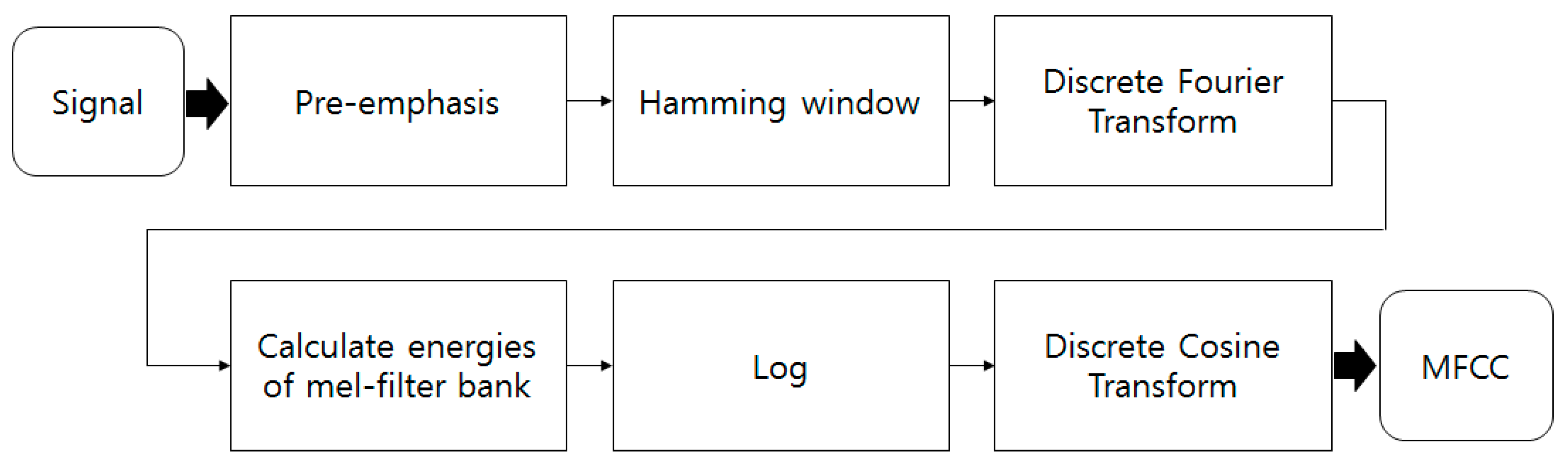
4.2. Experimental Results

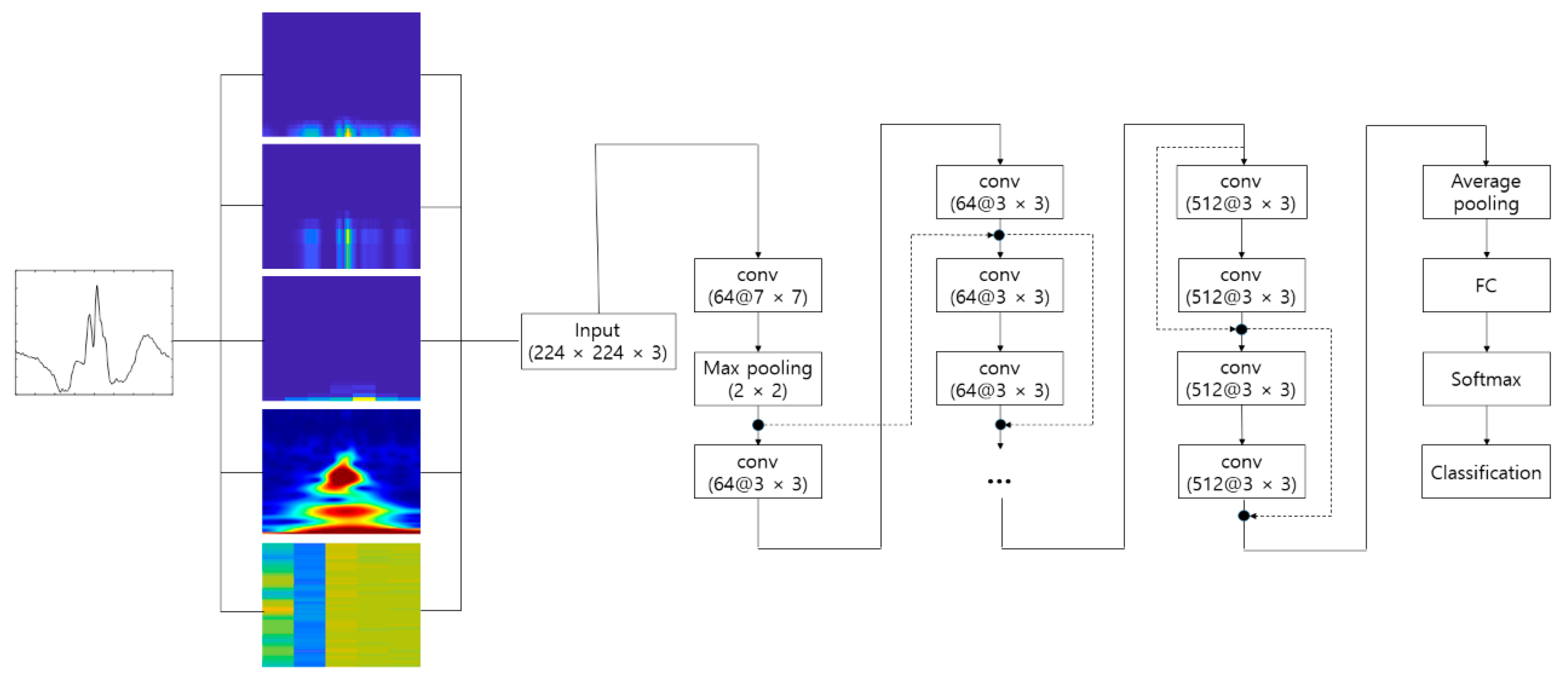
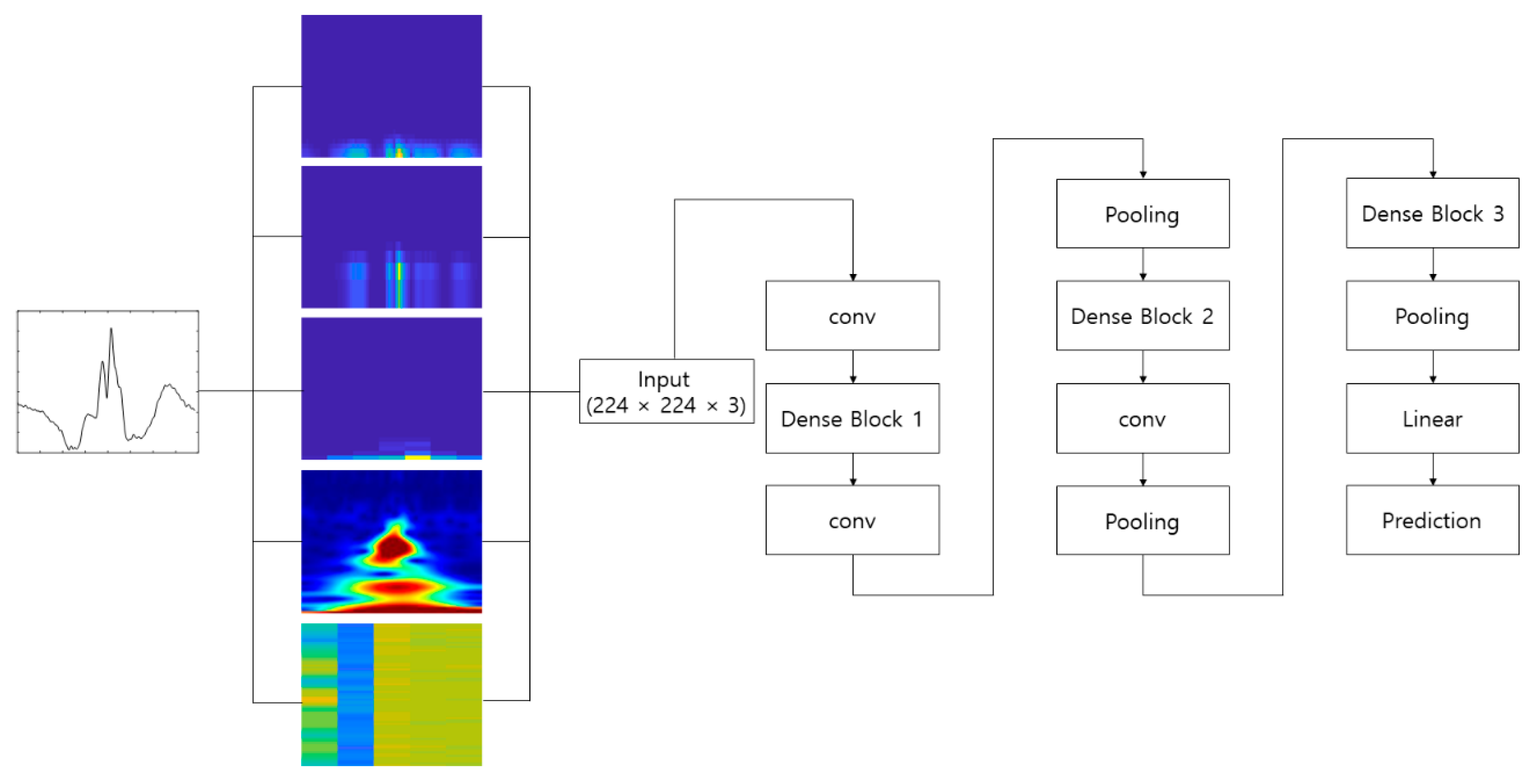
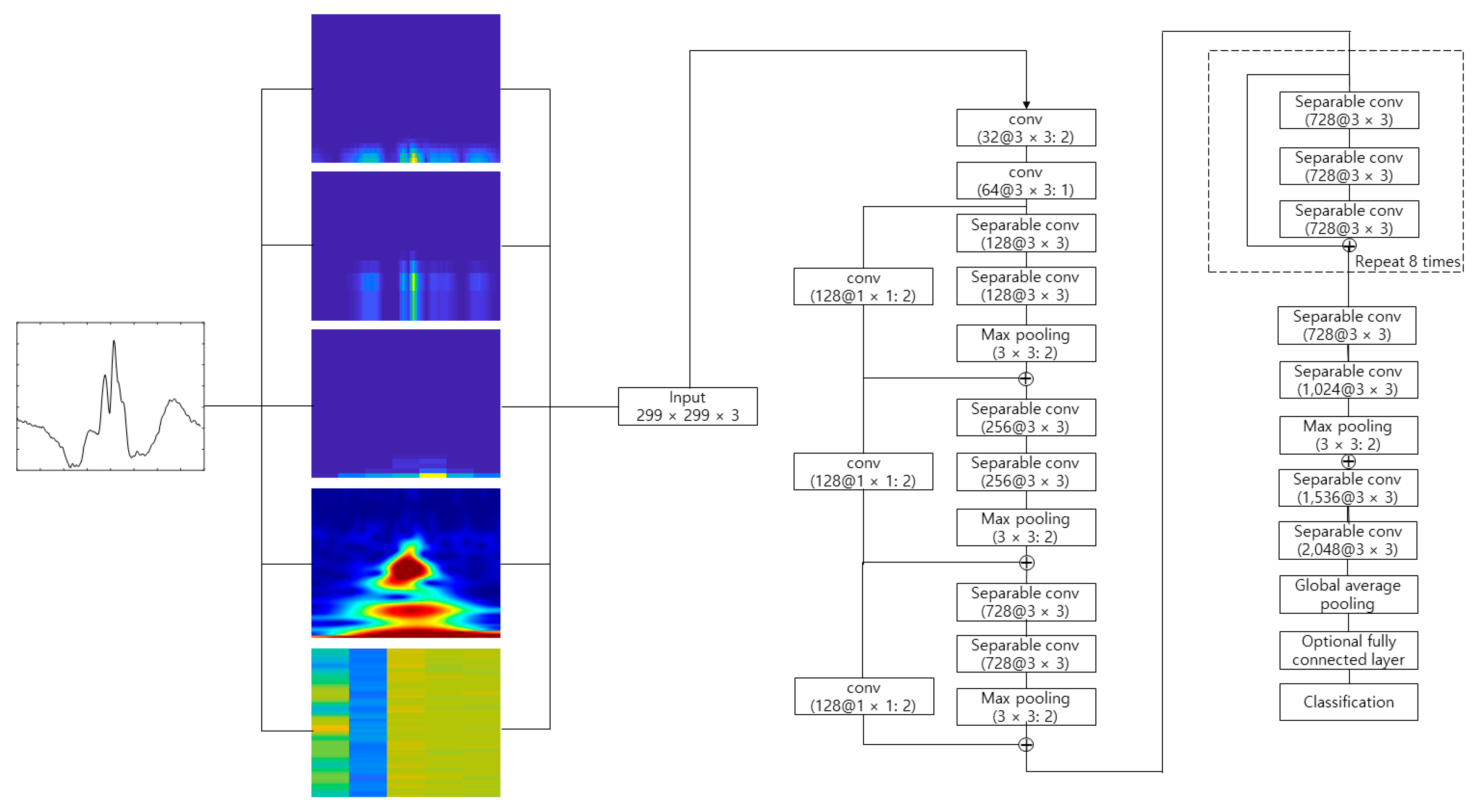
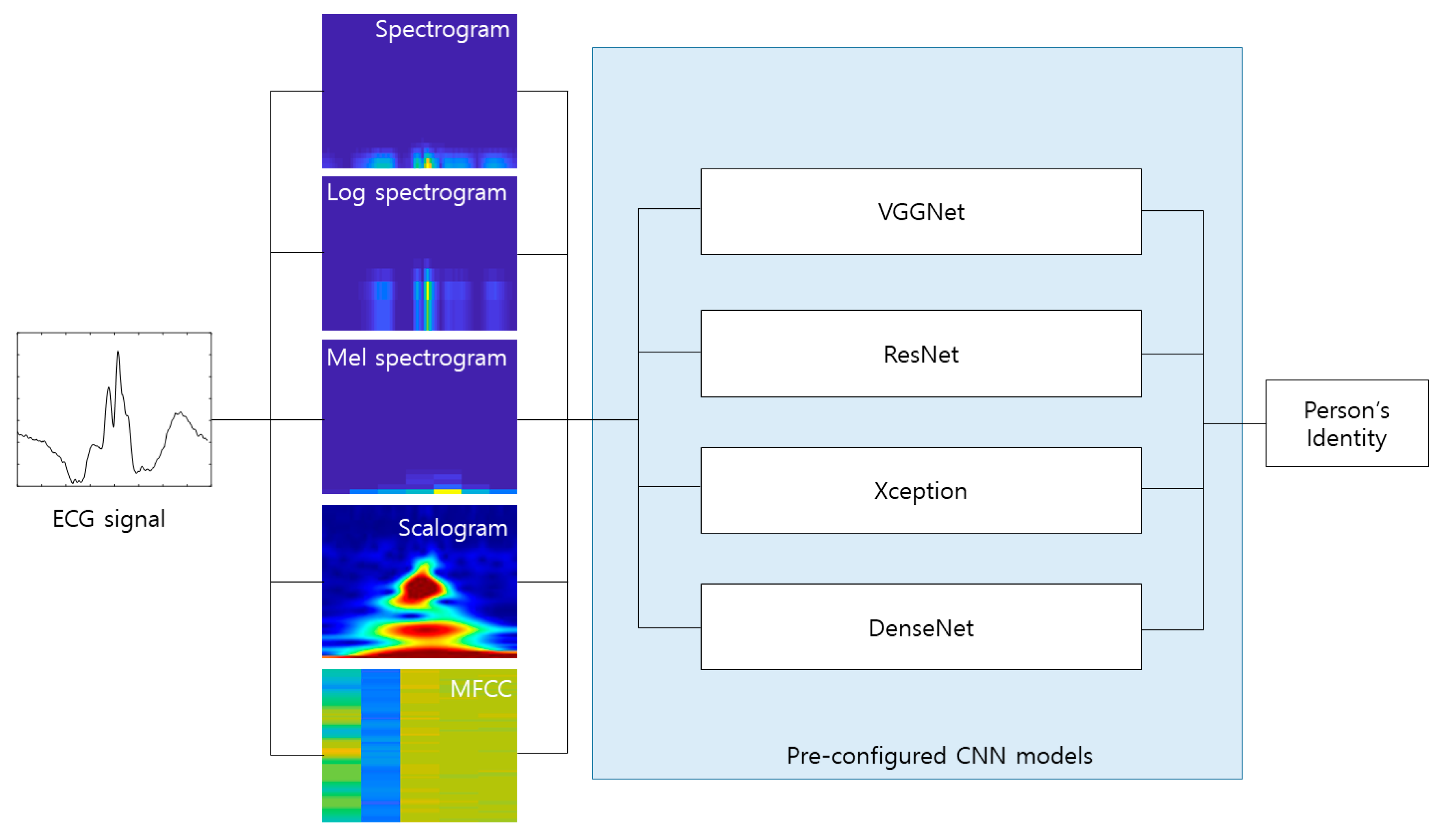
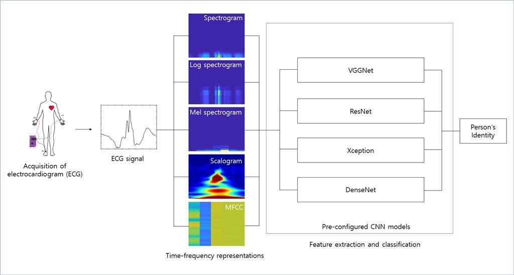
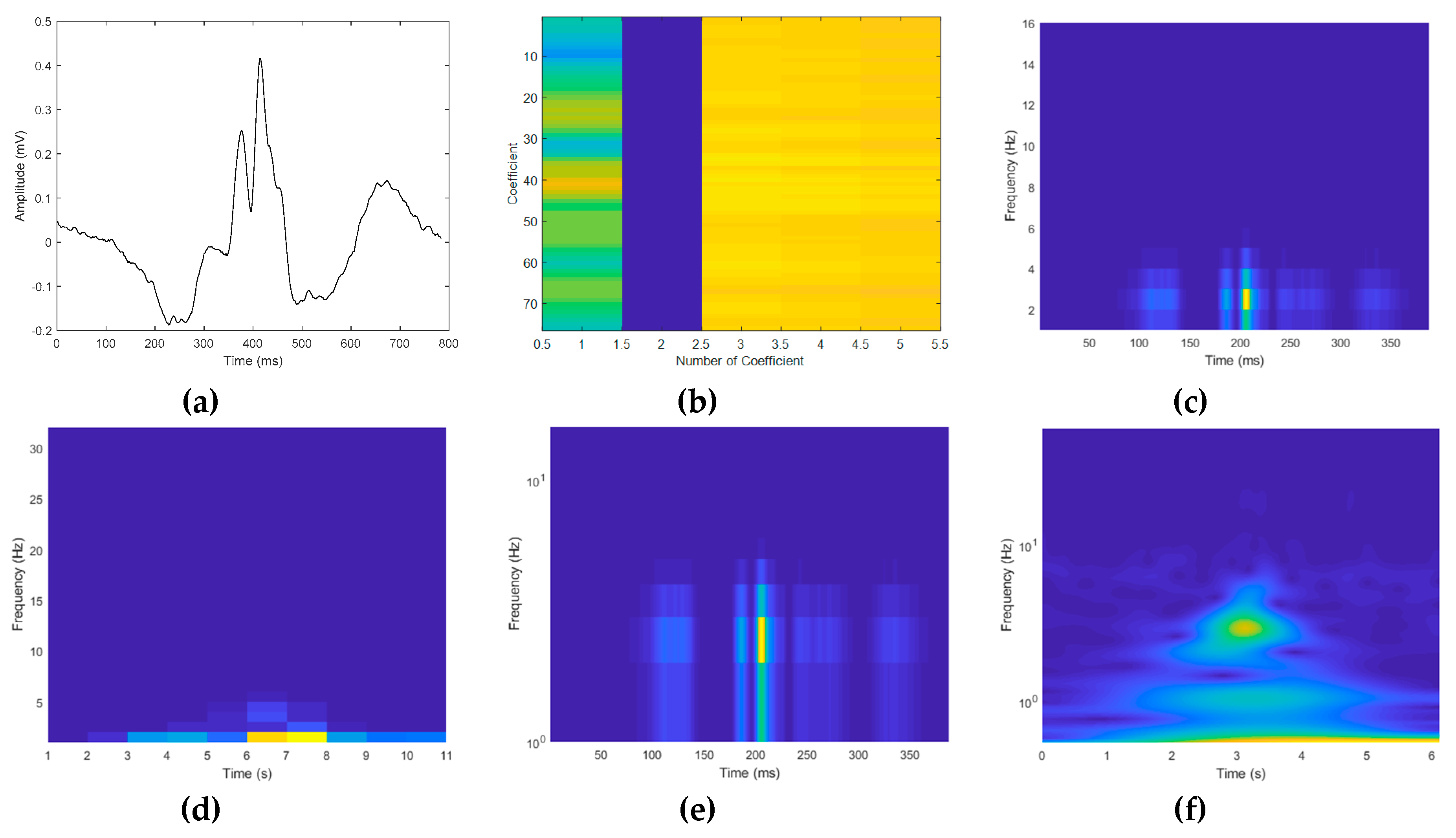
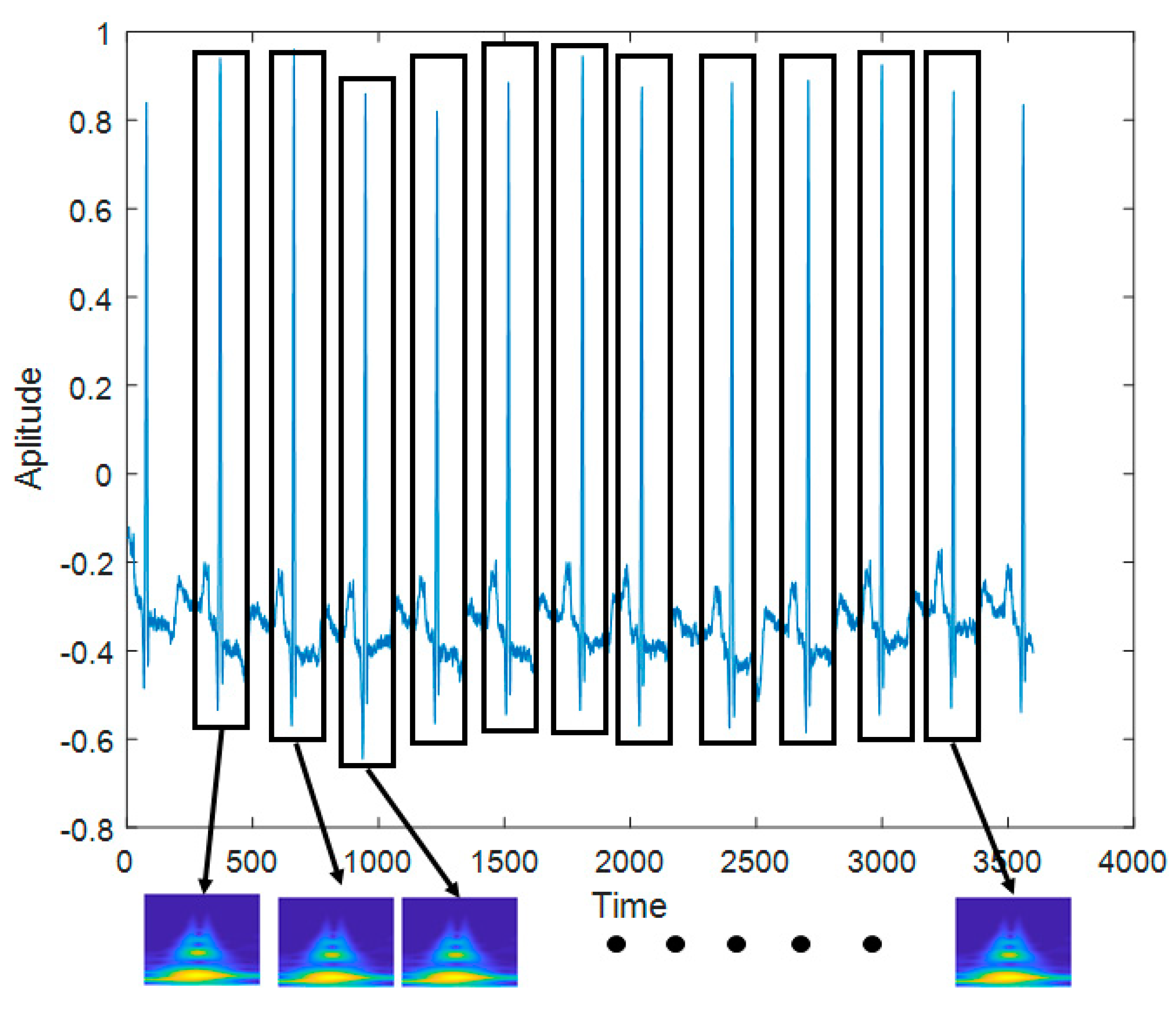
The experiment was performed using a computer with the following specifications: Nvidia GeForce GTX 1080 Ti, Intel i7-6850K central processing unit at 3.60 GHz, Windows 10 64-bit operating system, and 64 GB random-access memory. In this study, ECG biometrics using pre-configured models of the CNN with various time-frequency representations were evaluated. The signals were preprocessed to reduce the noise, and the R peak points were detected to normalize the center point of the ECG data. In other words, one data point was extracted based on each detected R peak point. However, the number of R peaks detected for each recording was different, as each person had a different heart rate, and the detection rate of the R peak was different for each signal. To construct the same amount of data for each class, the total number of R peak points detected for each class was calculated. The class was excluded when the number of detected R peaks was too small. When the number of detected R peaks was large, a few detected R peaks were removed to ensure the same amount of data in each class. Considering only the data from lead I, a frame length of 784 centered on the detected R peak point was obtained. The data were then transformed to the time-frequency representations. Here, the spectrogram, log spectrogram, mel spectrogram, scalogram, and MFCC were considered as the time-frequency representations. The transformed ECG data were 2D, which could be applied to the 2D CNNs. 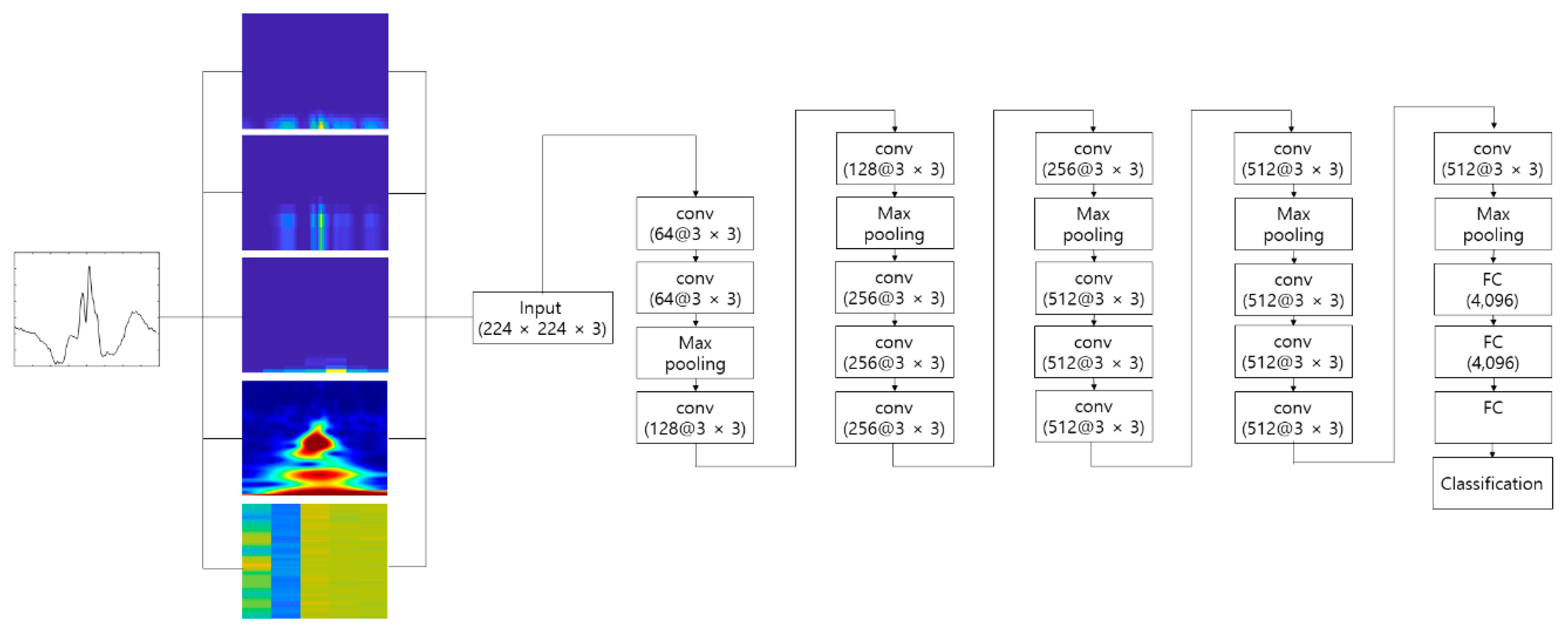Figure 10 shows the process of making the input image from the raw ECG signal. The pre-configured models based on the 2D CNN were the VGGNet, Xception, ResNet, and DenseNet models discussed earlier. The 2D ECG image was input to the CNN, and the neural network was trained to classify its identity. The depth of the neural network in the VGGNet, ResNet, and DenseNet models was 19, 101, and 201, respectively. We did not consider a potential issue from the variability from the selection of the ECG sensor devices. A different ECG sensor device (or product) would change the shape of the ECG signals and accuracy.

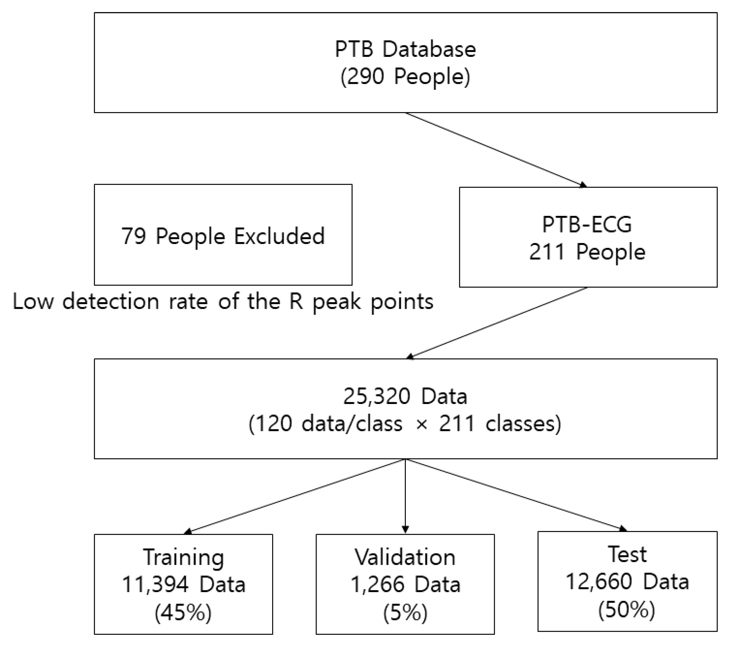
PTB-ECG is an open access database and includes ECG data from 290 people. However, the data from 211 people were used to construct the PTB-ECG database as the ECG data from the remaining 79 had only few R peak points. The R peak points from 211 people were compared and adjusted to ensure that the maximum number of data per class was 120. The database size of PTB-ECG was 784 × 25, 320 (120 data/class × 211 classes). The row refers to the dimension of the data, while the column indicates the number of data. To train the CNNs, PTB-ECG was divided into the training, validation, and test datasets with ratios of 0.45, 0.05, and 0.5, respectively. To shorten the training time, the training set was composed of 45% normally less than other literature works in the field of machine learning, and a larger ratio for the training set results in too high accuracy to compare performance. The sizes of the training, validation, and test datasets were 784 × 11,394, 784 × 1266, and 784 × 12,660, respectively. 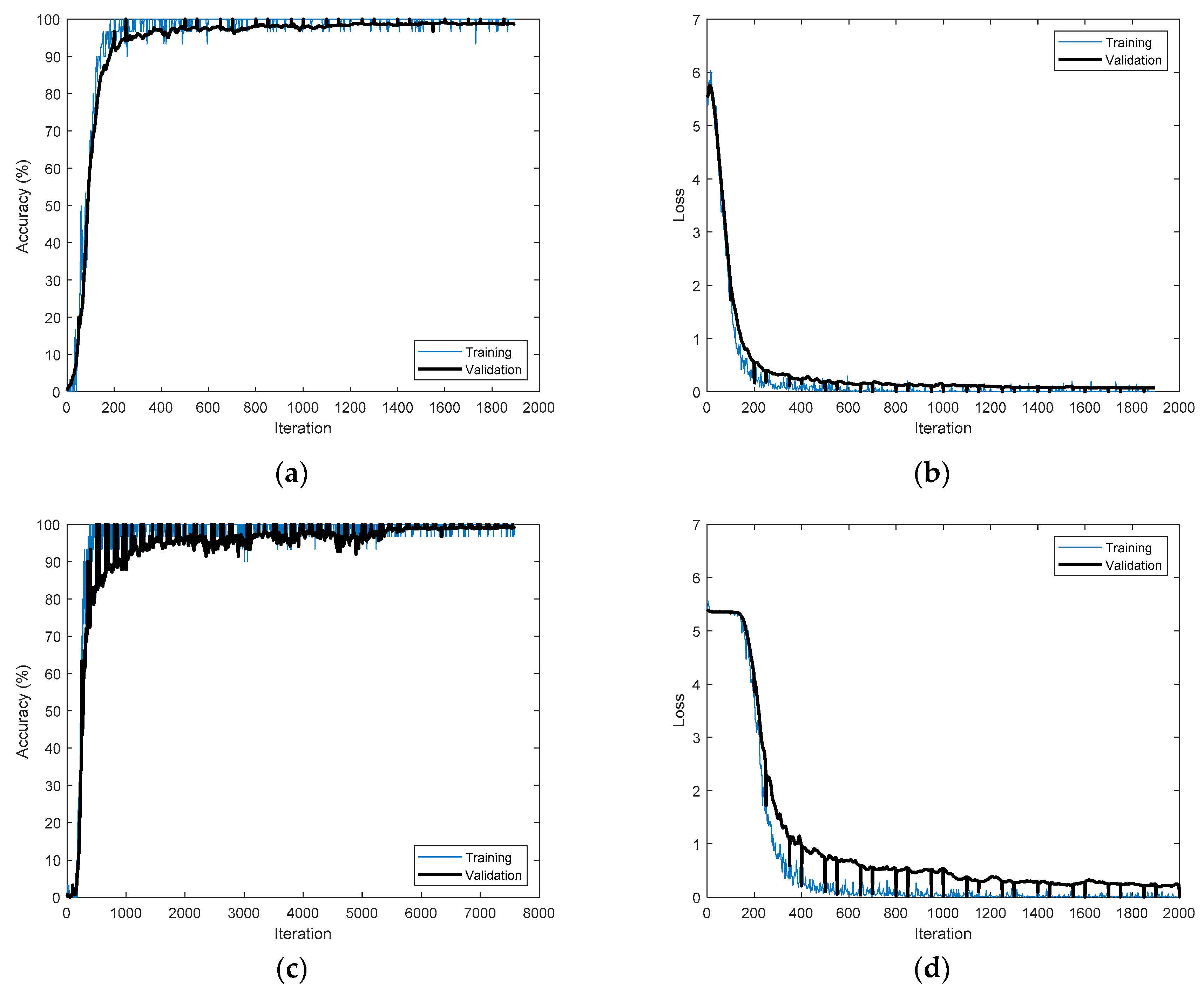Figure 11 shows the structure of PTB-ECG. The CNNs were trained using a mini-batch size of 30, an initial learning rate of 0.0001, the Adam (adaptive moment estimation) training optimizer, and an epoch varied according to the model. PCA (principle component analysis)-L2 was executed by entering vectors reshaped from the diminished input image and measuring Euclidean distance (L2). The PCA dimension was 20.

Table 1. Accuracies achieved by PCA-L2 using time-frequency representations on PTB-ECG.

Input Type	Model	Test Accuracy
MFCC	PCA-L2	97.59
Spectrogram		98.16
Log spectrogram		97.76
Mel spectrogram		97.76
Scalogram		97.96

shows the accuracies achieved by PCA-L2 using time-frequency representations on PTB-ECG. PCANet [42] is a neural network that has a CNN architecture based on PCA. PCANet was executed with 4 as the patch size, 4 filters, 4 as the block size, and 0.5 as the block overlap ratio.

Table 2. Accuracies achieved by PCANet using time-frequency representations on PTB-ECG.

Input Type.	Model	Accuracy
		Training	Test
MFCC	PCANet	99.72	98.56
Spectrogram		99.72	98.15
Log spectrogram		99.70	98.74
Mel spectrogram		99.78	98.37
Scalogram		99.78	98.89

shows the accuracies achieved by PCANet using time-frequency representations on PTB-ECG.

Table 3. Accuracies achieved by various models based on the CNN using different time-frequency representations on PTB-ECG.

Input Type	Model	Epoch	Accuracy
			Training	Validation	Test
MFCC	VGGNet-19	20	0.47	0.47	0.47
	Xception	20	99.72	99.45	98.84
	ResNet-101	20	99.46	99.13	97.84
	DenseNet-201	5	99.77	99.61	98.99
Spectrogram	VGGNet-19	20	98.80	97.71	96.58
	Xception	20	99.76	99.53	98.85
	ResNet-101	20	99.57	99.37	98.08
	DenseNet-201	5	98.90	98.50	97.83
Log spectrogram	VGGNet-19	20	98.03	96.52	94.99
	Xception	20	99.18	98.50	97.16
	ResNet-101	20	99.45	97.95	96.79
	DenseNet-201	5	97.12	95.26	94.38
Mel spectrogram	VGGNet-19	20	95.08	91.00	89.11
	Xception	20	98.68	98.18	96.92
	ResNet-101	20	97.80	98.42	96.85
	DenseNet-201	5	97.48	96.92	95.98
Scalogram	VGGNet-19	20	98.46	98.66	97.02
	Xception	20	98.75	98.82	97.33
	ResNet-101	20	99.43	98.74	97.83
	DenseNet-201	5	99.13	98.74	97.16

presents the accuracies achieved by the different models based on CNN using time-frequency representations on PTB-ECG. Considering MFCC on PTB-ECG, CNN failed to train VGGNet-19. The best accuracies achieved by the time-frequency representations on PTB-ECG were 98.99% for DenseNet-201 in MFCC, 98.85% for Xception in spectrogram, 97.16% for Xception in log spectrogram, 96.92% for Xception in mel spectrogram, and 97.83% for ResNet-101 in scalogram. This paper did not consider a potential issue from the variability from the selection of the ECG sensor devices. A different ECG sensor device (or product) would change the shape of the ECG signals and accuracy. The MFCC input to the DenseNet-201 model achieved the best accuracy for the PTB-ECG dataset. 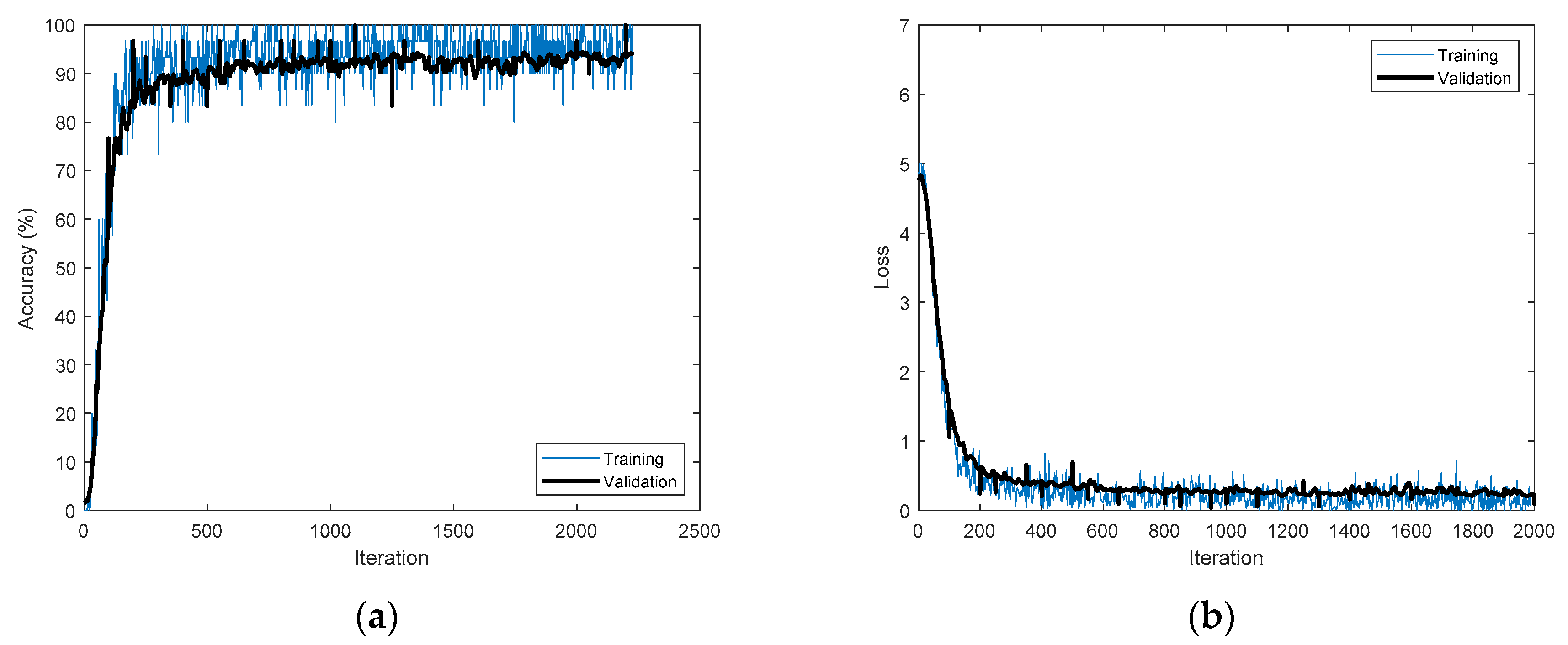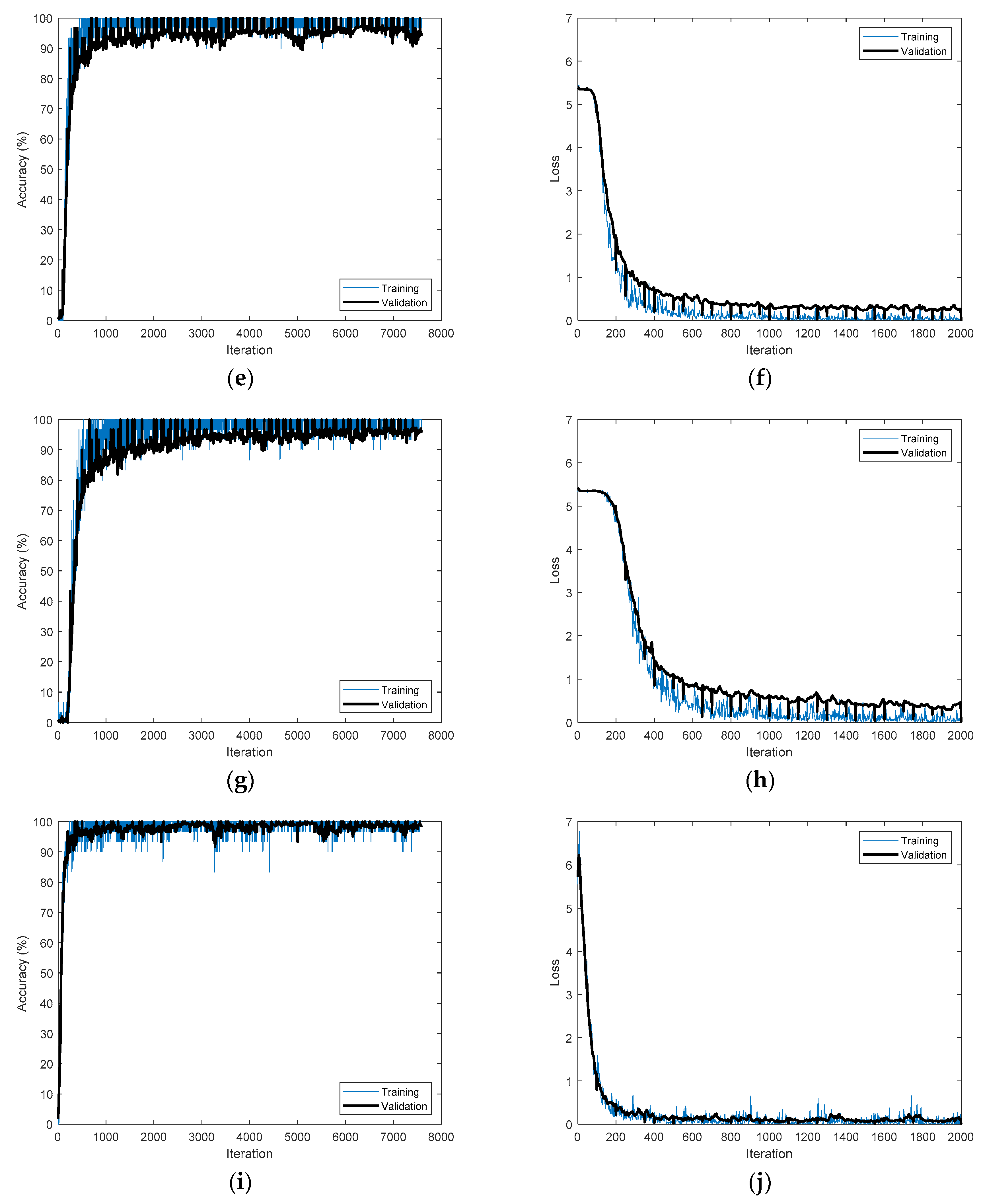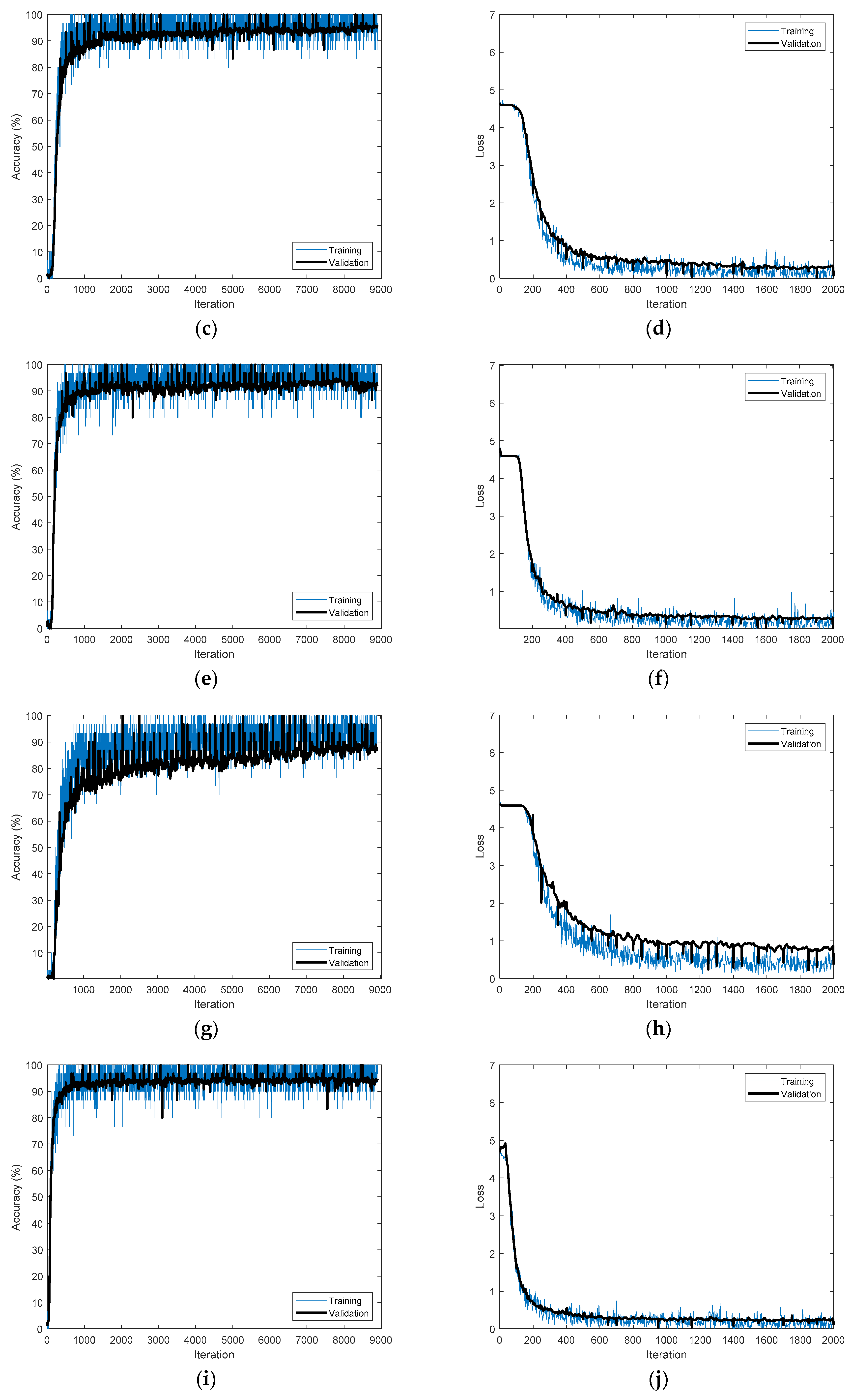Figure 12 shows the training processes that achieved the best accuracies for the time-frequency representations applied to PTB-ECG.

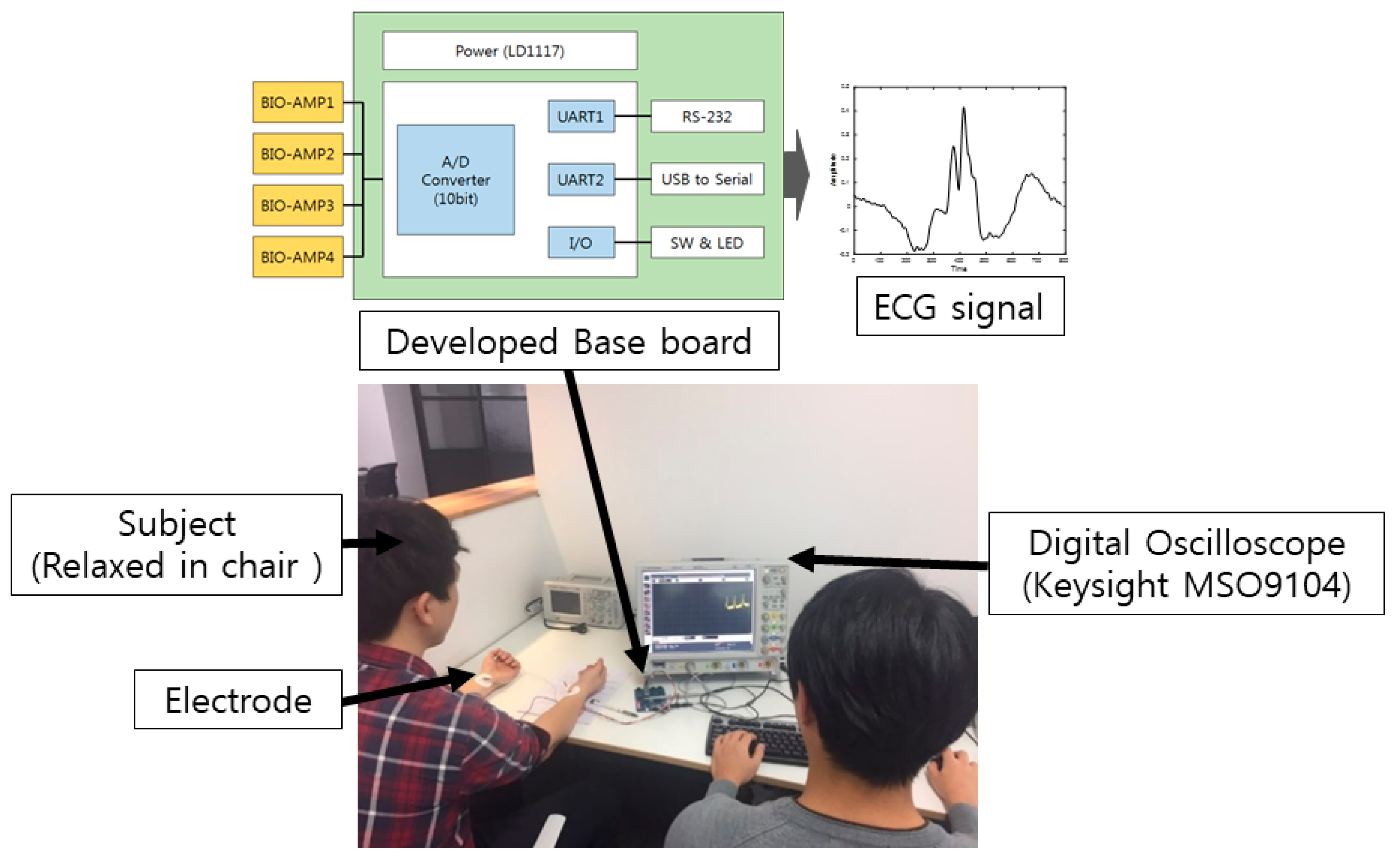
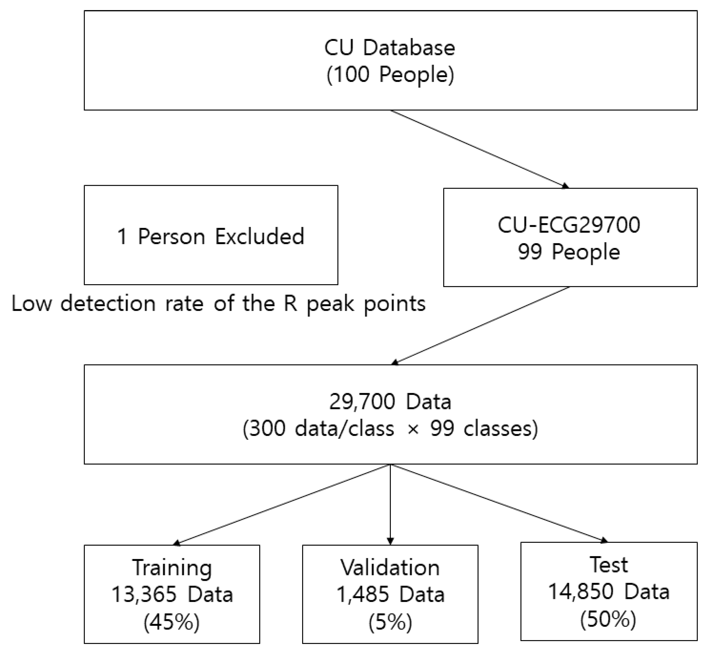
The CU database directly constructed for this study was acquired at 500 kHz. The dataset was resampled to 1 kHz because it was too large for data processing. The CU database included ECG data from 100 people. However, the data from 99 people were used to construct CU-ECG as the ECG data from one subject had very few R peak points. The R peak points from 99 people were compared and adjusted to ensure that the maximum number of data per class was 300. The size of the CU-ECG database was 784 × 29,700 (300 data/class × 99 classes). The row represents the dimension of the data, while the column indicates the number of data. To train the CNNs, CU-ECG was divided into the training, validation, and test datasets with ratios of 0.45, 0.05, and 0.5, respectively. The sizes of the training, validation, and test datasets were 784 × 13,365, 784 × 1485, and 784 × 14,850, respectively. Figure 13 shows the structure of CU-ECG. The CNNs were trained using a mini-batch size of 30, an initial learning rate of 0.0001, the Adam training optimizer, and an epoch varied according to the model. PCA-L2 was executed by entering vectors reshaped from the diminished input image and measuring Euclidean distance. The PCA dimension was 20.

Table 4. Accuracies achieved by PCA-L2 using time-frequency representations on CU-ECG.

Input Type	Model	Test Accuracy
MFCC	PCA-L2	90.36
Spectrogram		89.41
Log spectrogram		86.43
Mel spectrogram		87.39
Scalogram		90.14

shows the accuracies achieved by PCA-L2 using time-frequency representations on CU-ECG. PCANet was executed with 4 as the patch size, 4 filters, 4 as the block size, and 0.5 as the block overlap ratio.

Table 5. Accuracies achieved by PCANet using time-frequency representations on CU-ECG.

Input Type	Model	Accuracy
		Training	Test
MFCC	PCANet	96.05	89.88
Spectrogram		95.99	90.88
Log spectrogram		96.03	89.94
Mel spectrogram		95.99	89.10
Scalogram		95.92	92.29

shows the accuracies achieved by PCANet using time-frequency representations on CU-ECG.

Table 6. Accuracies achieved by various models based on the CNN using time-frequency representations on CU-ECG.

Input Type	Model	Epoch	Accuracy
			Training	Validation	Test
MFCC	VGGNet-19	20	93.35	90.24	86.21
	Xception	20	96.07	95.56	93.62
	ResNet-101	20	95.56	95.15	92.46
	DenseNet-201	5	96.17	95.08	93.82
Spectrogram	VGGNet-19	20	91.95	91.99	87.87
	Xception	20	96.01	95.62	94.03
	ResNet-101	20	95.69	94.48	91.64
	DenseNet-201	5	94.71	94.01	91.83
Log spectrogram	VGGNet-19	20	93.76	91.92	87.56
	Xception	20	95.26	93.80	90.65
	ResNet-101	20	94.01	92.53	89.29
	DenseNet-201	5	93.92	92.79	88.75
Mel spectrogram	VGGNet-19	20	88.80	89.29	86.28
	Xception	20	92.65	91.99	88.84
	ResNet-101	20	91.55	91.45	88.42
	DenseNet-201	5	90.76	90.03	86.77
Scalogram	VGGNet-19	20	93.55	93.60	90.56
	Xception	20	95.68	95.56	93.49
	ResNet-101	20	95.71	94.75	92.11
	DenseNet-201	5	95.58	95.08	92.84

presents the accuracies achieved by the different models based on the CNN using time-frequency representations on CU-ECG. The best accuracies achieved by the time-frequency representations on CU-ECG were 93.82% for DenseNet-201 in MFCC, 94.03% for Xception in spectrogram, 90.65% for Xception in log spectrogram, 88.84% for Xception in mel spectrogram, and 93.49% for Xception in scalogram. The spectrogram input to the Xception model achieved the best accuracy for the CU-ECG dataset. Figure 14 shows the training processes that achieved the best accuracies for the different time-frequency representations applied to CU-ECG.

The MIT(Massachusetts Institute of Technology)-BIH(Beth Israel Hospital) arrhythmia database consists of ECG signals from 48 subjects. The data had a sample rate of 360 Hz and a 10 s length. Most data had the MLII (Modified Limb lead II) signal except two subjects. Therefore, MLII data from 46 subjects were used for biometrics. Noise was eliminated from the signal, and the R peaks were detected by the Pan–Tompkins algorithm. The number of detected R peaks was small because the length of MIT-BIH arrhythmia had a short length signal. The R peak points from 46 people were compared and adjusted to ensure that the maximum number of data per class was five. Data were captured with 289 samples putting the R peak as the center. The size of the MIT-BIH-arrhythmia-ECG database was 289 × 230 (5 data/class × 46 classes). The row represents the dimension of the data, while the column indicates the number of data. To train the CNNs, MIT-BIH-arrhythmia-ECG was divided into the training and test datasets with ratios of 0.6 and 0.4, respectively. The sizes of the training and test datasets were 289 × 138 and 289 × 92, respectively. The CNNs were trained using a mini-batch size of 10, an initial learning rate of 0.0001, a max epoch of 5, and the Adam training optimizer. PCA-L2 was executed by entering vectors reshaped from the diminished input image and measuring Euclidean distance. The PCA dimension was 20.

Table 7. Accuracies achieved by PCA-L2 using time-frequency representations on MIT (Massachusetts Institute of Technology)-BIH (Beth Israel Hospital)-arrhythmia-ECG.

Input Type	Model	Test Accuracy
MFCC	PCA-L2	4.35
Spectrogram		1.09
Log spectrogram		2.17
Mel spectrogram		3.26
Scalogram		1.09

shows the accuracies achieved by PCA-L2 using time-frequency representations on MIT-BIH-arrhythmia-ECG. PCANet was executed with 4 as the patch size, 4 filters, 4 as the block size, and 0.5 as the block overlap ratio.

Table 8. Accuracies achieved by PCANet using time-frequency representations on MIT-BIH-arrhythmia-ECG.

Input Type	Model	Accuracy
		Training	Test
MFCC	PCANet	100	78.26
Spectrogram		100	89.13
Log spectrogram		100	86.96
Mel spectrogram		100	82.61
Scalogram		100	86.96

shows the accuracies achieved by PCANet using time-frequency representations on MIT-BIH-arrhythmia-ECG.

Table 9. Accuracies achieved by various models based on the CNN using different time-frequency representations on MIT-BIH-arrhythmia-ECG.

Input Type	Model	Epoch	Accuracy (%)
			Training	Validation
MFCC	VGGNet-19	5	2.17	2.17
	Xception	5	2.17	5.43
	ResNet-101	5	18.12	22.83
	DenseNet-201	5	66.67	48.91
Spectrogram	VGGNet-19	5	2.9	2.17
	Xception	5	14.49	8.7
	ResNet-101	5	36.96	38.04
	DenseNet-201	5	75.36	63.04
Log spectrogram	VGGNet-19	5	2.17	2.17
	Xception	5	94.06	70.65
	ResNet-101	5	86.96	72.83
	DenseNet-201	5	97.10	84.78
Mel spectrogram	VGGNet-19	5	2.17	2.17
	Xception	5	2.9	5.43
	ResNet-101	5	24.64	32.61
	DenseNet-201	5	50.72	38.04
Scalogram	VGGNet-19	5	3.62	4.35
	Xception	5	96.38	67.39
	ResNet-101	5	96.38	67.39
	DenseNet-201	5	99.28	75.00

presents the accuracies achieved by the different models based on CNN using time-frequency representations on MIT-BIH-arrhythmia-ECG. The best accuracies achieved by the time-frequency representations on MIT-BIH-arrhythmia-ECG were 48.91% for DenseNet-201 in MFCC, 63.04% for DenseNet-201 in spectrogram, 84.78% for DenseNet-201 in log spectrogram, 38.04% for DenseNet-201 in mel spectrogram, and 75.00% for DenseNet-201 in scalogram. The log spectrogram input to the DenseNet-201 model achieved the best accuracy for the MIT-BIH-arrhythmia-ECG dataset. There were some cases of learning failure because the size of the dataset was too small.

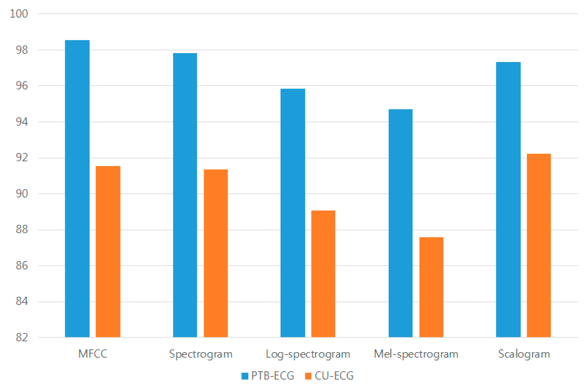
The mean accuracies of the different time-frequency representations applied to PTB-ECG were 98.56% for MFCC, 97.84% for spectrogram, 95.83% for log spectrogram, 94.72% for mel spectrogram, and 97.34% for scalogram. The mean accuracies of the different time-frequency representations applied to the CU-ECG were 91.53% for MFCC, 91.34% for spectrogram, 89.06% for log spectrogram, 87.58% for mel spectrogram, and 92.25% for scalogram. The mean accuracies of PTB-ECG and CU-ECG corresponding to the time-frequency representations were 95.04% for MFCC, 94.59% for spectrogram, 92.45% for log spectrogram, 91.15% for mel spectrogram, and 94.79% for scalogram. The MFCC accuracies were 0.45%, 2.60%, 3.90%, and 0.25% higher than the spectrogram, log spectrogram, mel spectrogram, and scalogram accuracies, respectively. Figure 15 shows a comparison between the accuracies of the different time-frequency representations.

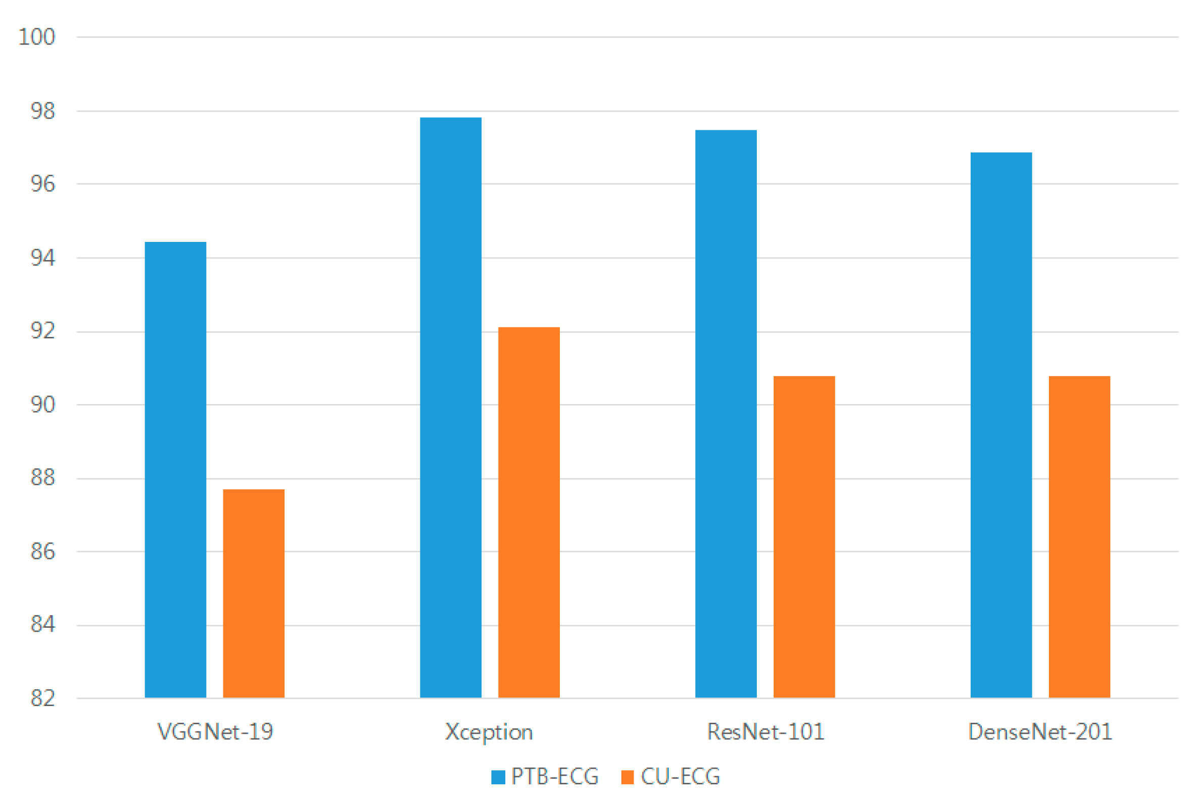
The mean accuracies of the different models in PTB-ECG were 94.43% for VGGNet-19, 97.82% for Xception, 97.48% for ResNet-101, and 96.87% for DenseNet-201. The mean accuracies of the different models in CU-ECG were 87.70% for VGGNet-19, 92.13% for Xception, 90.78% for ResNet-101, and 90.80% for DenseNet-201. The mean accuracies of PTB-ECG and CU-ECG for the different models were 91.06% for VGGNet-19, 94.97% for Xception, 94.13% for ResNet-201, and 93.84% for DenseNet-201. The Xception accuracies were 3.91%, 0.84%, and 1.14% higher than the VGGNet-19, ResNet-101, and DenseNet-201 accuracies, respectively. Figure 16 shows a comparison between the accuracies of various models based on the CNN. The mean accuracies of PCA-L2 and PCANet were 97.81 and 98.54 in PTB-ECG, 88.75 and 90.42 in CU-ECG, and 2.4 and 84.78 in MIT-BIH-arrhythmia-ECG, respectively. The Xception in PTB-ECG was 0.1% higher than PCA-L2 and 0.72% lower than PCANet. The Xception in CU-ECG was 3.38% and 1.71% higher than PCA-L2 and PCANet, respectively.

5. Conclusions

We evaluated ECG biometrics using pre-configured models of CNNs with various time-frequency representations. Biometrics technology records a person’s physical or behavioral characteristics in a digital signal via a sensor and analyzes it to identify the person. Biometrics offer great convenience to human lifestyles throughout society. An ECG signal is obtained by detecting and amplifying a minute electrical signal flowing on the skin using a noninvasive electrode when the heart muscle depolarizes at each heartbeat. In biometrics, the ECG is especially advantageous in security applications because the heart is located within the body and moves while the subject is alive. However, a few body states generate noisy biometrics. The analysis of signals in the frequency domain has a robust effect on the noise. As the ECG is noise-sensitive, various studies have applied time-frequency transformations that are robust to noise, with CNNs achieving a good performance in image classification. Various studies have applied the time-frequency representations of 1D ECG signals to 2D CNNs. Combinations of the time-frequency representations and CNN deep models have not been investigated. In this study, we employed MFCC, spectrogram, log spectrogram, mel spectrogram, and scalogram time-frequency transforms and the VGGNet, GoogLeNet, ResNet, and DenseNet deep CNN models. The PTB-ECG and CU-ECG databases were used in this study. The MFCC accuracies were 0.45%, 2.60%, 3.90%, and 0.25% higher than the spectrogram, log spectrogram, mel spectrogram, and scalogram accuracies, respectively. The Xception accuracies were 3.91%, 0.84%, and 1.14% higher than the VGGNet-19, ResNet-101, and DenseNet-201 accuracies, respectively. The mean accuracies of PCA-L2 and PCANet were 97.81 and 98.54 in PTB-ECG, 88.75 and 90.42 in CU-ECG, and 2.4 and 84.78 in MIT-BIH-arrhythmia-ECG, respectively. The Xception in PTB-ECG was 0.1% higher than PCA-L2 and 0.72% lower than PCANet. The Xception in CU-ECG was 3.38% and 1.71% higher than PCA-L2 and PCANet, respectively. The Xception with time-frequency representation showed close accuracy in PTB-ECG, which was easily successfully classified. However, the Xception outperformed other methods in CU-ECG, which was not easily successfully classified. Further studies would focus on new and better time-frequency representations.

References

1. Mobarakeh, A.K.; Carrillo, J.A.C.; Aguilar, J.J.C. Robust face recognition based on a new supervised kernel subspace learning method. Symmetry 2019, 19, 1643. [Google Scholar] [CrossRef] [PubMed]
2. Zhang, Y.; Juhola, M. On biometrics with eye movements. IEEE J. Biomed. Health Inform. 2017, 21, 1360–1366. [Google Scholar] [CrossRef] [PubMed]
3. Boles, W.W. A security system based on human iris identification using wavelet transform. In Proceedings of the First International Conference on Conventional and Knowledge based Intelligent Electronics Systems, Adelaide, Australia, 21–23 May 1997; pp. 533–541. [Google Scholar]
4. Jain, A.K.; Arora, S.S.; Cao, K.; Best-Rowden, L.; Bhatnagar, A. Fingerprint recognition of young children. IEEE Trans. Inf. Forensics Secur. 2017, 12, 1505–1514. [Google Scholar] [CrossRef]
5. Wang, H.; Hu, J.; Deng, W. Compressing fisher vector for robust face recognition. IEEE Access. 2017, 5, 23157–23165. [Google Scholar] [CrossRef]
6. Pokhriyal, N.; Tayal, K.; Nwogu, I.; Govindaraju, V. Cognitive-biometric recognition from language usage: A feasibility study. IEEE Trans. Inf. Forensics Secur. 2017, 12, 134–143. [Google Scholar] [CrossRef]
7. Nguyen, B.P.; Tay, W.L.; Chui, C.K. Robust biometric recognition from palm depth images for gloved hands. IEEE Trans. Human-Machi. Syst. 2015, 45, 799–804. [Google Scholar] [CrossRef]
8. Xu, W.; Lee, E.J. A Hybrid method based on dynamic compensatory fuzzy neural network algorithm for face recognition. Int. J. Control. Autom. Syst. 2014, 12, 688–696. [Google Scholar] [CrossRef]
9. Lin, C.; Kumar, A. Matching contactless and contact-based convolutional fingerprint images for biometrics identification. IEEE Trans. on Image Process. 2018, 27, 2008–2021. [Google Scholar] [CrossRef] [PubMed]
10. Jang, Y.K.; Kang, B.J.; Kang, R.P. A novel portable iris recognition system and usability evaluation. Int. J. Control. Autom. Syst. 2010, 8, 91–98. [Google Scholar] [CrossRef]
11. Hong, S.J.; Lee, H.S.; Tho, K.A.; Kim, E.T. Gait recognition using multi-bipolarized contour vector. Int. J. Control. Autom. Syst. 2009, 7, 799–808. [Google Scholar] [CrossRef]
12. Kim, M.J.; Kim, W.Y.; Paik, J.K. Optimum geometric transformation and bipartite graph-based approach to sweat pore matching for biometric identification. Symmetry 2018, 10, 175. [Google Scholar] [CrossRef]
13. Yang, J.; Sun, W.; Liu, N.; Chen, Y.; Wang, Y.; Han, S. A novel multimodal biometrics recognition model based on stacked ELM and CCA methods. Symmetry 2018, 10, 96. [Google Scholar] [CrossRef]
14. Korshunov, P.; Marcel, S. Impact of score fusion on voice biometrics and presentation attack detection in cross-database evaluations. IEEE J. Sel. Top. Signal. Process. 2017, 11, 695–705. [Google Scholar] [CrossRef]
15. Zhang, L.; Cheng, Z.; Shen, Y.; Wang, D. Palmprint and palmvein recognition based on DCNN and a new large-scale contactless palmvein dataset. Symmetry 2018, 10, 78. [Google Scholar] [CrossRef]
16. Tolosana, R.; Vera-Rodriguez, R.; Fierrez, J.; Ortega-Garcia, J. Exploring recurrent neural networks for on-line handwritten signature biometrics. IEEE Access 2018, 6, 5128–5138. [Google Scholar] [CrossRef]
17. Gahi, Y.; Lamrani, M.; Zoglat, A.; Guennoun, M.; Kapralos, B.; El-Khatib, K. Biometric identification system based on electrocardiogram data. In Proceedings of the New Technologies, Mobility and Security, Tangier, Morocco, 5–7 November 2008; pp. 1–4. [Google Scholar]
18. Byeon, Y.H.; Lee, J.N.; Pan, S.B.; Kwak, K.C. Multilinear eigenECGs and FisherECGs for individual identification from information obtained by an electrocardiogram sensor. Symmetry 2018, 10, 487. [Google Scholar] [CrossRef]
19. Chen, K.C.; Chien, P.C. A fast ECG diagnosis using frequency-based compressive neural network. In Proceedings of the IEEE Global Conference on Consumer Electronics, Nagoya, Japan, 24–27 October 2017; pp. 1–2. [Google Scholar]
20. Akdeniz, F.; Kayikçioğlu, T. Detection of ECG arrhythmia using large Choi Williams time-frequency feature set. In Proceedings of the Medical Technologies National Congress, Trabzon, Turkey, 12–14 October 2017; pp. 1–4. [Google Scholar]
21. Sharma, R.R.; Kumar, M.; Pachori, R.B. Joint time-frequency domain-based CAD disease sensing system using ECG signals. IEEE Sens. J. 2019, 19, 3912–3920. [Google Scholar] [CrossRef]
22. Zhao, Z.; Liu, C.; Li, Y.; Li, Y.; Wang, J.; Lin, B.S.; Li, J. Noise rejection for wearable ECGs using modified frequency slice wavelet transform and convolutional neural networks. IEEE Access 2019, 7, 34060–34067. [Google Scholar] [CrossRef]
23. Aviña-Cervantes, J.G.; Torres-Cisneros, M.; Martinez, J.E.S.; Pinales, J. Frequency, time-frequency and wavelet analysis of ECG signal. In Proceedings of the Multiconference on Electronics and Photonics, Guanajuato, Mexico, 7–10 November 2006; pp. 257–261. [Google Scholar]
24. Zhang, Q.; Zhou, D.; Zeng, X. PulsePrint: Single-arm ECG biometric human identification using deep learning. In Proceedings of the IEEE Annual Ubiquitous Computing, Electronics and Mobile Communication Conference, New York, NY, USA, 19–21 October 2017; pp. 452–456. [Google Scholar]
25. Luz, E.J.D.S.; Moreira, G.J.P.; Oliveira, L.S.; Schwartz, W.R.; Menotti, D. Learning deep off-the-person heart biometrics representations. IEEE Trans. Inf. Forensics Secur. 2018, 13, 1258–1270. [Google Scholar]
26. Deshmane, M.; Madhe, S. ECG based biometric human identification using convolutional neural network in smart health applications. In Proceedings of the Fourth International Conference on Computing Communication Control and Automation, Pune, India, 16–18 August 2018; pp. 1–6. [Google Scholar]
27. Wu, J.; Liu, C. Research on personal identity verification based on convolutional neural network. In Proceedings of the IEEE International Conference on Information and Computer Technologies, Kahului, HI, USA, 14–17 March 2019; pp. 57–64. [Google Scholar]
28. Simonyan, K.; Zisserman, A. Very deep convolutional networks for large-scale image recognition. Comput. Sci. 2015, arXiv:1409.1556v6. [Google Scholar]
29. Chollet, F. Xception: Deep learning with depthwise separable convolutions. Comput. Sci. 2017, arXiv:1610.02357v3. [Google Scholar]
30. He, K.; Zhang, X.; Ren, S.; Sun, J. Deep residual learning for image recognition. In Proceedings of the IEEE Conference on Computer Vision and Pattern Recognition, Las Vegas, NV, USA, 27–30 June 2016; pp. 770–778. [Google Scholar]
31. Huang, G.; Liu, Z.; Maaten, L.V.D.; Weinberger, K.Q. Densely connected convolutional networks. Comput. Sci. 2018, arXiv:1608.06993v5. [Google Scholar]
32. Israel, S.A.; Irvine, J.M.; Cheng, A.; Wiederhold, M.D.; Wiederhold, B.K. ECG to identify individuals. Pattern Recognit. 2005, 38, 133–142. [Google Scholar] [CrossRef]
33. Towhid, S.; Rahman, M. Spectrogram segmentation for bird species classification based on temporal continuity. In Proceedings of the 20th International Conference of Computer and Information Technology, Dhaka, Bangladesh, 22–24 December 2017; pp. 22–24. [Google Scholar]
34. Meng, H.; Yan, T.; Yuan, F.; Wei, H. Speech emotion recognition from 3D log-mel spectrograms with deep learning network. IEEE Access 2016, 4, 1–14. [Google Scholar] [CrossRef]
35. Xu, M.; Duan, L.Y.; Cai, J.; Chia, L.T.; Xu, C.; Tian, Q. HMM-based audio keyword generation. In Advances in Multimedia Information Processing - PCM 2004, Proceedings of Pacific-Rim Conference on Multimedia; Aizawa, K., Nakamura, Y., Satoh, S., Eds.; Springer: Heidelberg, Berlin, 2004; pp. 566–574. [Google Scholar]
36. Shi, L.; Ahmad, I.; He, Y.J.; Chang, K.H. Hidden Markov model based drone sound recognition using MFCC technique in practical noisy environments. J. Commun. Netw. 2018, 20, 509–518. [Google Scholar] [CrossRef]
37. Khorrami, H.; Moavenian, M. A comparative study of DWT, CWT and DCT transformation in ECG arrhythmias classification. Expert Syst. Appl. 2010, 37, 5751–5757. [Google Scholar] [CrossRef]
38. Li, T.; Zhou, M. ECG classification using wavelet packet entropy and random forests. Entropy 2016, 18, 285. [Google Scholar] [CrossRef]
39. Goldberger, A.L.; Amaral, L.N.; Glass, L.; Hausdorff, J.M.; Ivanov, P.C.; Mark, R.G.; Mietus, J.E.; Moody, G.B.; Peng, C.K.; Stanley, H.E. PhysioBank, PhysioToolkit, and PhysioNet: Components of a new research resource for complex physiologic signals. Circulation 2000, 101, e215–e220. [Google Scholar] [CrossRef] [PubMed]
40. Wubbeler, G.; Stavridis, M.; Kreiseler, D.; Bousseljot, R.D.; Elster, C. Verification of humans using the electrocardiogram. Pattern Recognit. Lett. 2007, 28, 1172–1175. [Google Scholar] [CrossRef]
41. Choi, H.S.; Lee, B.H.; Yoon, S.R. Biometric authentication using noisy electrocardiograms acquired by mobile sensors. IEEE Access 2016, 4, 1266–1273. [Google Scholar] [CrossRef]
42. Lee, J.N.; Byeon, Y.H.; Pan, S.B.; Kwak, K.C. An EigenECG network approach based on PCANet for personal identification from ECG signal. Sensors 2018, 18, 4024. [Google Scholar] [CrossRef] [PubMed]
Figure 1. Structure of VGGNet with the time-frequency representations as inputs.
Applsci 09 04810 g001
Figure 2. Structure of ResNet with the time-frequency representations as inputs.
Applsci 09 04810 g002
Figure 3. Structure of DenseNet with the time-frequency representations as inputs.
Applsci 09 04810 g003
Figure 4. Structure of Xception with the time-frequency representations as inputs.
Applsci 09 04810 g004
Figure 5. Scale mappings of the log and mel transforms; (a) Log; (b) Mel.
Applsci 09 04810 g005
Figure 6. Process used to calculate MFCC.
Applsci 09 04810 g006
Figure 7. Time-frequency representation: (a) original signal; (b) MFCC; (c) spectrogram; (d) mel spectrogram; (e) log spectrogram; (f) scalogram.
Applsci 09 04810 g007
Figure 8. ECG biometrics using several time-frequency representations.
Applsci 09 04810 g008
Figure 9. Environment for acquiring the Chosun University (CU)-ECG signals.
Applsci 09 04810 g009
Figure 10. Process of making the input image from the raw ECG signal.
Applsci 09 04810 g010
Figure 11. Structure of Physikalisch-Technische Bundesanstalt (PTB)-ECG employed in this study.
Applsci 09 04810 g011
Figure 12. Training processes that achieved the best accuracies for the time-frequency representations applied to PTB-ECG. (a) Accuracy of DenseNet-201 using MFCC; (b) loss of DenseNet-201 using MFCC; (c) accuracy of Xception using spectrogram; (d) loss of Xception using spectrogram; (e) accuracy of Xception using log spectrogram; (f) loss of Xception using log spectrogram; (g) accuracy of Xception using mel spectrogram; (h) loss of Xception using mel spectrogram; (i) accuracy of ResNet-101 using scalogram; (j) loss of ResNet-101 using scalogram.
Applsci 09 04810 g012aApplsci 09 04810 g012b
Figure 13. Structure of CU-ECG.
Applsci 09 04810 g013
Figure 14. Training processes that achieved the best accuracies for the time-frequency representations applied to CU-ECG. (a) Accuracy of DenseNet-201 using MFCC; (b) loss of DenseNet-201 using MFCC; (c) accuracy of Xception using spectrogram; (d) loss of Xception using spectrogram; (e) accuracy of Xception using log spectrogram; (f) loss of Xception using log spectrogram; (g) accuracy of using Xception mel spectrogram; (h) loss of Xception using mel spectrogram; (i) accuracy of Xception using scalogram; (j) loss of Xception using scalogram.
Applsci 09 04810 g014aApplsci 09 04810 g014b
Figure 15. Comparison between the mean accuracies of the different time-frequency representations.
Applsci 09 04810 g015
Figure 16. Comparison between the mean accuracies of various models based on CNN.
Applsci 09 04810 g016