Predicting Students Success in Blended Learning—Evaluating Different Interactions Inside Learning Management Systems

Abstract

Algorithms and programming are some of the most challenging topics faced by students during undergraduate programs. Dropout and failure rates in courses involving such topics are usually high, which has raised attention towards the development of strategies to attenuate this situation. Machine learning techniques can help in this direction by providing models able to detect at-risk students earlier. Therefore, lecturers, tutors or staff can pedagogically try to mitigate this problem. To early predict at-risk students in introductory programming courses, we present a comparative study aiming to find the best combination of datasets (set of variables) and classification algorithms. The data collected from Moodle was used to generate 13 distinct datasets based on different aspects of student interactions (cognitive presence, social presence and teaching presence) inside the virtual environment. Results show there are no statistically significant difference among models generated from the different datasets and that the counts of interactions together with derived attributes are sufficient for the task. The performances of the models varied for each semester, with the best of them able to detect students at-risk in the first week of the course with AUC ROC from 0.7 to 0.9. Moreover, the use of SMOTE to balance the datasets did not improve the performance of the models.

1. Introduction

Student dropout and failure are two major problems faced during the teaching-learning process of computer programming at any education level [1]. These disciplines have high failure rates around the world, sometimes achieving over 50% [1,2,3,4,5]. According to the literature, many factors may contribute to this low approval rate, such as difficulties related to the required abstraction for the proper development of algorithms, difficulties in problem-solving, and also the early stage, in which the programming courses are placed inside the curricula [6,7,8].

In Brazil, for example, there is a huge demand for Information Technology (IT) professionals but the formal teaching-learning environments (schools, courses, universities, etc.) do not account for this demand. The prediction of the IT professionals demand is around 70,000 between 2020 and 2024 [9] but the Brazilian universities are graduating 46 thousand, which leaves a deficit of 24,000 per year. In other parts of the world, the scenario is heavier. It estimates that the deficit of IT professionals in Europe from 2015 until 2020 is roughly 800,000 [10,11].

Beside that market demand, international institutes and organisms consider the computational thinking a knowledge for future generation [12,13]. Resnik [14] says that the consumption of technology by the actual generation do not convert them, automatically, in technology producers or developers. The author state that this generation must understand how technology works to create, update and innovate in hardware, software and so on.

In this context, the early identification of at-risk students can help the educational staff to take some action to mitigate the students’ failure. One of the biggest challenges is to develop algorithms and tools to predict the students’ behavior, aiming to facilitate the intervention of professors, tutors and educators [15,16].

Educational Data Mining (EDM) is an interdisciplinary research area that deals with the development of methods and techniques to explore data from educational contexts and which has been exploring different techniques to detect at-risk students [17].

Interactions within the learning management systems are used in several works to extract knowledge and discover patterns [18]. For example, Murray et al. [19] shows that the students with the highest rates of access to the study materials within the Learning Management Systems (LMS) received highest grades, and Dickson [20] presents that the number of clicks made by a student is strongly correlated to its final grade in the course.

At the same time that there is an overwhelming amount of studies about the detection of at-risk students, most of the results reported in the literature do not show solutions able of detecting at-risk students until the middle of the course [21]. In this work, the collected data belongs to the whole course (15 weeks) but the prediction is based only on the first 8 weeks of the course.

Nevertheless, in this paper we also compare different types of interactions that took place within the LMS and it is based according to a conceptual framework proposed by Garrison et al. [22]. The authors proposed a framework to identify the critical elements required for a successful computer-mediated educational experience [22]. The critical elements identified are: (1) cognitive presence—representing the extent to which one is able to construct meaning; (2) social presence—representing the ability that the student has to project himself to the others participants of the virtual community as a real person and (3) teaching presence—being the design of an educational experience, facilitating and enhancing cognitive and social presence for the achievement of learning outcomes.

According to Swan [23], each of the critical elements proposed by Garrison et al. [22] represents different types of students’ interaction in the LMS. These interactions can affect learning efficiency, that is, with the course (cognitive presence), among peers (social presence) and with teachers/instructors (teaching presence).

In this context, the main goal of this paper is to evaluate whether the use of these three different types of presences significantly influences in the performance of predictive models to early detect at-risk students. To achieve this goal, we evaluate whether a given type of presence in the LMS is more suitable to early predict at-risk students or the data collected through a survey may help to improve the performance of the models.

Since the number of samples is small and unbalanced, we needed to find a solution to overcome this problem. Previous studies have shown that the use of the SMOTE (Synthetic Minority Over-sampling Technique)technique to balance datasets helps on improving the performance of the models [24]. As we are dealing with highly unbalanced datasets, we also applied SMOTE balancing technique to check if its use interferes in the models’ performance.

Before initiating the courses, social and demographic data were collected from the students. Since we get only the interaction count from Moodle logs, we included this information in the study to evaluate to which extent this information could help to improve the performances of the models. We base our studies on previous work that use solely the count of interactions to predict students at-risk, with the justification of using information that is not restricted to a given type of learning management system [25]. The idea here is to test the sole use of the interaction count to see if it achieves a satisfactory result.

In this work, we do not distinguish our analysis between students’ failure and dropout. Therefore, if it is not explicitly said the difference, the term “at-risk students” means students that got a final grade lower than 6.0 (on a scale from 1.0 to 10.0). In this context, students who dropped out got zero in their final grade and, consequently, are included in this definition.

For those reasons, the present work come up with the following research questions:

RQ1. 

Which are the most appropriate datasets to early predict at-risk students?

RQ2. 

Is the sole use of the count of students interactions sufficient to early predict students’ failure in the course?

RQ3. 

Does the use of oversampling techniques (SMOTE) help the models to achieve better performances?

RQ4. 

Does the use of data from questionnaires applied at the beginning of the course help to improve model performance?

The remainder of this paper is divided into 4 sections—Section 2 presents related works. Section 3 presents the methodology, the process of data collection, its description, the dataset generation and the model evaluation. Section 4 reports the results obtained in this study and Section 5 shows the works’ conclusion and discussion.

2. Related Work

Predicting at-risk students on higher education is a relatively well-established task in the literature, as well as the notion of interactions within the LMS. Some works show that students’ performance has often been associated with different measures of LMS interactions and usually has a high correlation with their success in the course. This section presents a non-exhaustive review of the literature that used user interaction data to predict at-risk students.

2.1. Programming Courses

In introductory programming course context, Costa et al. [24] presented a comparative study aiming to measure the effectiveness of educational data mining techniques aiming on predicting at-risk students. The results have shown that the techniques used in the study can identify students with the risk of failing, where the best results were achieved using the Support Vector Machine (SVM) algorithm. Azcona et al. [26] present a research methodology to detect at-risk students in computer programming courses too. The authors provide adaptive feedback to students based on weekly generated predictions. The models used students’ offline data and information about the activity logs. Results show that the students who followed the personalized guidance and recommendations performed better in exams. The usage of online learning material (in an introductory programming course) was used to predict academic success [27]. The results obtained have shown that the time spent with the material is a moderate predictor of student success. The performances of the models depend on the amount of data used to train them (where the predictions become more accurate during the progress of the course).

2.2. Computer Science/IT Courses

In a computer science course, Tillmann et al. [28] used exam results data from the LMS to indicators of academic success. Results show that the use of data of domain-specific skills could help to improve the accuracy and student interaction data almost does not interfere in the results. Using interaction logs from three computer science courses, Sheshadri et al. [29] tried to predict students’ performance in a blended course. Results show that the performance can be predicted using data from LMS and also from a forum, version control and homework system. Using a plug-in to capture data from Moodle, Jokhan et al. [30] tried to predict the student’s performance in the first year of an IT literacy course. A regression model was used to determine if there is any correlation between students’ online behavior and performance. Results show that the performance in this course could be predicted based on their average logins per week and the average completion rates of activities.

2.3. University

On an university context, a model to early predict students who are at-risk of failing was presented by Sandoval et al. [31]. The data comes from the university’s LMS, that is, activity logs for each user and the administrative information system called DARA, that is, past and current academic status and demographic data. The results outperform other approaches in terms of accuracy, cost and generalization. In Mwalumbwe and Mtebe [32], the authors designed a Learning Analytics tool to determine the causation between LMS usage and students’ performance at Mbeya University of Science and Technology. Results show that discussion posts, peer interaction, and exercises are significant factors for students’ academic achievement in blended learning at the university.

2.4. Fully Online

On a fully online course, Hung et al. [33] used time-series clustering to early identify at-risk online students. Data were collected from an online graduate program in the United States, and results show that the proposed approach could generate models with higher accuracy if it is compared to traditional frequency aggregation approaches. In Soffer and Cohen [34], the authors used learning analytics methods on engagement data from online courses aiming to find their impact on academic achievements. Results showed that there are significant differences between who completes the course and who does not. An example is that the students who complete the course are twice more active than those who do not complete (except for forum activities). In Kostopoulos et al. [35] it was combined classification and regression algorithms for predicting students’ performance in a distance web-based course. When the results are compared with some machine learning methods, they show that the proposed model is accurate and remains comprehensive. Baneres et al. [36] propose to identify at-risk students using an adaptive predictive model based on students’ grades, trained for each course. They also present an early warning system using dashboards visualization for stakeholders. The results show the effectiveness of the approach on data coming from a fully online university’s LMS.

2.5. Blended Courses

In a blended course context, Conijn et al. [37] processed data from LMS on 17 courses. Results show that the performance of predictive models strongly varies across courses, even when they are generated with data collected from a single institution. In Sukhbaatar et al. [38], the authors used a decision tree analysis on LMS data with the goal of predict (until the middle of the semester) students that are at-risk of failing or dropout in a blended course. Results showed that this approach worked well to predict the dropouts. However, to predict students that are at risk of failing, the method presented a lousy performance.

2.6. Multiple Data Sources

In Adejo & Connolly [39], the authors compared the use of multiple data sources (student record system, LMS and survey) and different classification algorithms aiming to predict student’s academic performance. The main result is that using multiple data sources combined with an ensemble of classifierhigh accuracy in the s brought a high accuracy in the prediction of student performance. Umer et al. [40] used machine learning algorithms and the LMS data to predict students at-risk of failing. Results show that those data can be used to predict students’ outcomes. However, the count of activities alone is not enough. In other words, the combination of LMS data and assessment scores can improve the accuracy of prediction models. Olivé et al. [41] tried to find which students would likely submit their assignments on time based on LMS data until two days before the deadline. The main goal was to perform an early prediction of at-risk students. The authors added contextual information to improve their predictions using neural networks, achieving satisfactory results.

2.7. Only Interaction Data/Log Files

Using only course log files, in Cohen [42], the author used data accumulated in three academic course to check if student activity on course websites may assist in providing early identification of learner dropout. Results show that identifying the changes in student activity during the course period could help in detecting at-risk students. In Kondo et al. [43] was proposed an automatic method to detect at-risk students by using log data of the LMS. Experimental results indicated that using this log data, some characteristics of behavior about learning which affect the student outcomes can be detected. Also, by using interaction data from the LMS, Usman et al. [44] used EDM and pre-processing techniques to predict students’ performance. Results show that the Decision Tree achieved the best performance, followed by Naive Bayes and kNN. In Detoni et al. [25], the authors presented a methodology to classify students using only the interaction count in the LMS. Three machine learning methods were tested and results showed that the patterns in the data could provide useful information to classify at-risk students, allowing personalized activities, trying to avoid the student dropout. In Zhou et al. [45], the authors created a feature selection framework to pre-processing the data coming from internet access logs and generate models to predict the students’ performance. Results have shown that this approach can identify most of the high-risk students. Some online characteristics were also discovered and can help educational professionals to understand the relation between students’ internet use and academic performance.

2.8. Early Prediction

Aiming to find the optimal time in a course to apply an early warning system, the authors of Howard et al. [46] examined eight prediction methods to identify at-risk students. The course has a weekly continuous assessment and a large proportion of resources on the LMS. The results show that the optimal time to implement an early warning system is in weeks 5-6 (halfway through the semester). This way, the students can make changes in their study patterns. One of the objectives in Lu et al. [47] was to find the moment that the at-risk students could be predicted. For that, the authors used learning analytics and big educational data approach to predict the students’ performance on a blended calculus course. Results show that the performance can be predicted when one-third of the semester is complete. With a similar idea, the authors of Gray and Perkins [48] proposed a new descriptive statistic for student attendance and applied machine learning methods to create a predictive model. Results show how at-risk students can be identified as early as week three in the fall semester. Appendix A presents an overview of the main characteristics of the works discussed in this section.

2.9. Approach Novelty

The novelty of our approach is based on the extensive comparison of datasets and classification algorithms, resulting in 65 combinations (13 datasets and 5 classification algorithms). We also used pre-processing techniques (SMOTE) aiming to tackle the lack of samples to train and test the algorithms. Some questionnaire data were used to aggregate more information on the discussion, adding information like social and demographic variables on the analysis. We also used three types of presence (cognitive, teaching and social) aiming to generate more data to predict student at-risk of failing and according to an existing theory about how interactions work inside Virtual Learning Environments.

The idea of making early predictions is to find out as early as possible whether the student is at risk of failing. For that, from the data available, we used just those related to the weeks up to the half of the semester (week 8). In this way, we are testing models that can be used in time to provide information that can help professors to intervene in order to avoid students failure.

3. Methodology

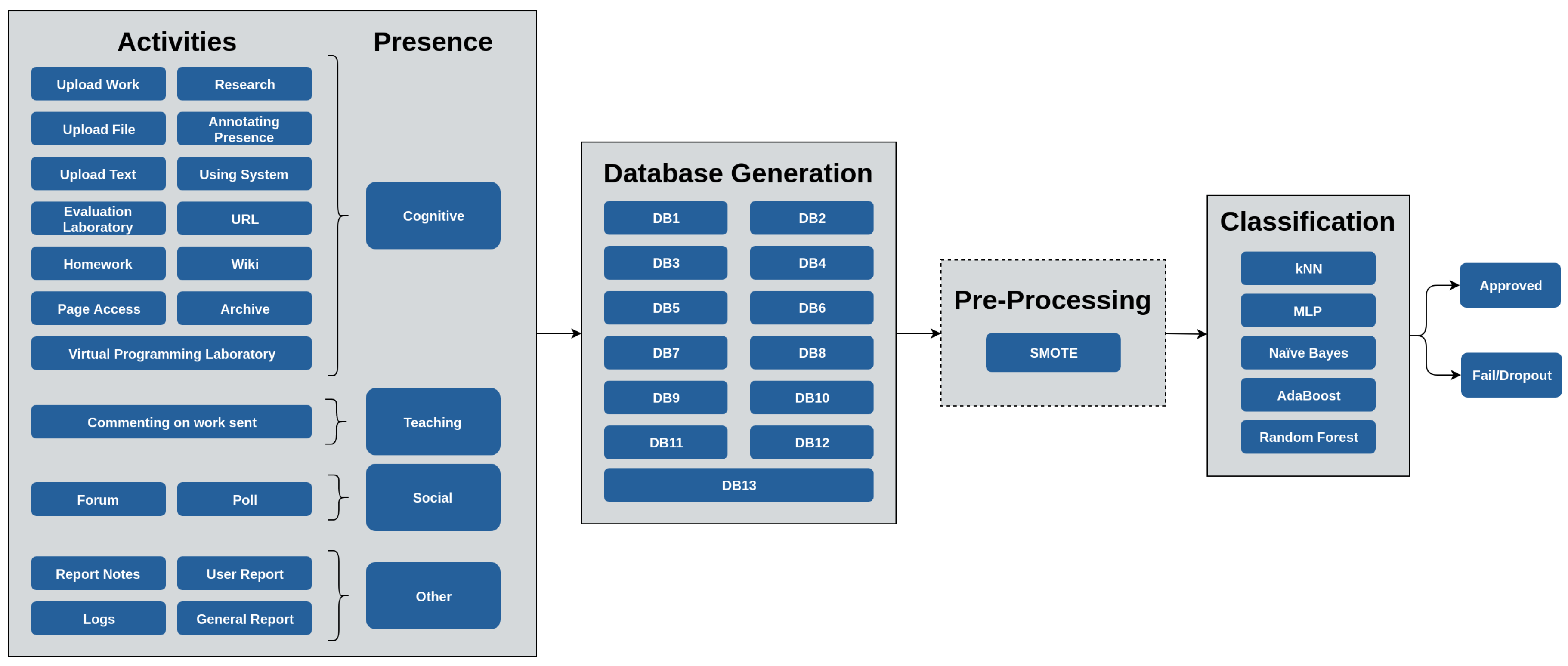
This section describes the methods used to achieve the goal of this paper. This research paper investigates thirteen different datasets (set of attributes), for each of the 4 (four) distinct semesters: 2016-1, 2016-2, 2017-1 and 2017-2, of an Introductory Programming Course to evaluate whether the types of presence, presented by Garrison et al. [22], influences in the performance of predictive models to early detect at-risk students. The overview of the adopted methodology is shown in Figure 1 and the four steps of the methodology are shown in Figure 2.

The first step consists of gathering data from Moodle logs, considering that the platform records the interactions that the students make in the VLE. The next step consists of generating the datasets containing different attributes to compare them and verify those which achieve the best results. Next, we employ some pre-processing techniques, such as oversampling, intending to increase the performance of the models. The fourth step consists of the generation and evaluation of the classification models. In the final step, we compare the obtained results to answer the research questions. The next subsections describe, in more detail, the steps followed.

3.1. Data Collection and Description

Data was collected from the Moodle logs of Introductory Programming courses of the Information and Communication Technologies (ICT) undergraduate program at the Federal University of Santa Catarina (UFSC). The introductory course is offered at ICT at night and it has 108 hours, in total, over 18 weeks. There are three classes per week, where one of them is an online activity. Every type of activity is computed as an “interaction”. In other words, independently of the type the activity (log in, click on a given link, send a file, etc.), the interaction count is incremented by one.

Table 1. Summary of data.

Semester	Interaction Count	Average of Interaction	Students Approved	Students Reproved	Total of Students
2016-1	10,395	547.10	6	13	19
2016-2	11,512	605.89	6	13	19
2017-1	23,457	902.19	9	17	26
2017-2	33,727	1349.08	12	13	25

shows the summary of the data.

The Average of Interaction is calculated by the Interaction Count divided by the Total of Students. The lecturer was the same for all four semesters. It is important to note that in 2016, the C programming language was used but in 2017 we started teaching the Python programming language. The activities were gradually developed by the lecturer for each semester and he also instead content from previous semester.

For example, every semester, the old exams are posted in the course. In 2017-1 (first semester of 2017), the lecturer posted new programming exercises, video classes and a bunch of links to other video classes and content. The LMS course became more abundant in the material than before. At the end of the course, in 2017-1, the lecturer created a new LMS course environment, reorganizing the topics and content, describing the environment to assist the student in following instructions and making the course very attractive to the student. In addition to the video classes and content, most of the activities cited here are related to programming exercises that can be developed, executed and evaluated in Moodle by the Virtual Programming Laboratory plugin (VPL) [49].

For all the courses, throughout the semester students had three assessments. In 2016-1 students had two tests—week 10 and 17 and a final assignment in week 18. The tests were handwriting, that is, students did not make it in VPL because the modified Moodle environment for tests (Moodle’s Test) that prohibits students access to the internet, was not available at the campus. In 2016-2 the Moodle’s test was installed and students had two VPL tests in weeks 8 and 16 and a final assignment in week 15. In 2017-1 students had two VPL tests in week 10 and week 16 and a final assignment in week 17. In 2017-2, it was a bit different, students had three VPL tests in weeks 9, 15 and 17.

It is important to note that in both semesters of 2016, the final assignment was made by a group of maximum 3 students, it was implemented at home, in 4 weeks and posted in Moodle. In 2017-1, the assignment was made by two students per group in two classes (the same double in both days). In 2017-2, all the tests were made within VPL in classes. The final score is calculated as follows: $FS=(T1\ast 0.35+T2\ast 0.35+ASGMT\ast 0.3)$, where FS is the final score, T1 and T2 are tests and ASGMT is the final assignment or the final test in 2017-2.

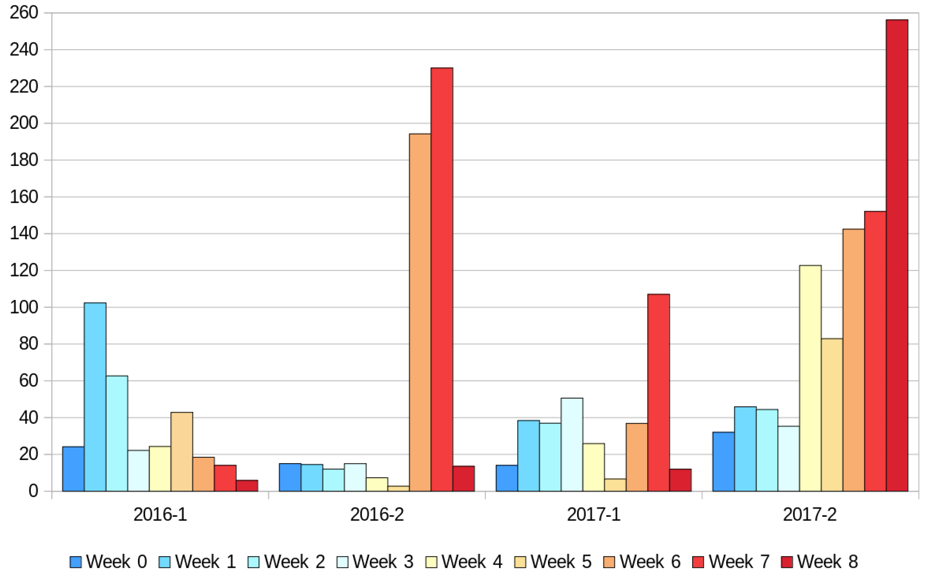
Every student interaction in the LMS is saved in the logs together with the description of the activity performed. From that, we calculated the interaction counting for each week during the course for every student. Figure 3 shows a frequency distribution of interactions on each week of the four semesters considered for this work. Regarding the weeks when the first test was applied, it is important to note that one or two weeks before the test, there was a peak of interactions, as seen in 2016-2, 2017-1 and 2017-2. It is also interesting that the students did not use the Moodle in 2016-1, even though there were 53 not-mandatory VPL activities there.

In 2016-1, there is not a peak per se. But the highest number of interaction happens on Week 1. For 2016-2 and 2017-1, most of the interaction happens on Week 7. The 2017-2 semester has the highest number of interactions, where the peak is found on Week 8. From the interactions, we generated thirteen datasets with different sets of derived attributes to compare the performances of the models.

Table 2. Description of the attributes.

Attribute	Description
Count	Interaction count for each week
Average	Average of interactions on the week
Median	Median of interactions on the week
Zeroed weeks [50]	Number of weeks with zero interactions until the moment
Average of the difference [50]	Average of the difference between interactions on week i and week $i+1$
Commitment factor [50]	Ratio between the student’s week interactions and the average class interaction for that week
Cognitive count [23]	Number of cognitive interaction on the week
Teaching count [23]	Number of teaching interaction on the week
Social count [23]	Number of social interaction on the week
Other count	Number of other types of interaction on the week

shows the description of the attributes generated.

It is important to point out that each attribute in Table 2 is gathered at student level, that is, every calculation in based on data collected for each student. Cognitive Count, Teaching Count and Social Count are the counting of the Cognitive, Teaching and Social Presences presented in Swan [23]. “Other count” is a category created by us for all the other interactions that do not fit the three previously mentioned categories. In other words, the sum of these four types of interactions result in $Coun{t}_i$ (Equation (1)).

Table 3. Example of interactions classification.

Attribute	Description
Cognitive count	Interactions involving content access and visualization: File upload/download, VPL exercise, URL access
Teaching count	Interactions with the professor: comments to the files sent
Social count	Interactions with other students: forum participation

presents how different interactions inside Moodle fall into the three types of presence evaluated in our work.

Students interactions are normally highly correlated to engagement in distance learning settings, reflecting the behaviour students have in relation the their course. According to Moore [51], the interaction with content (cognitive presence), interaction with instructors (teaching presence) and interaction among peers (social presence) are the three kinds of interactivity that affect the learning process. Each of these interaction types supports learning and in practice, none of them works independently [23]. The idea of using these types of interaction is to better discriminate each type of interaction aiming to help on the generation of better predictive models, that better capture students behaviour in those learning settings. The implicit idea is that students who fail present different interactions in the different types of presence than students who succeed and that difference helps to generate better models.

Following, we formalize every attribute contained in the datasets.

$$Coun{t}_i=\sum _{j=1}^7{x}_j.$$

(1)

Equation (1) represents the sum of interactions on every day j in each week i.

$$Averag{e}_i=\frac{{\sum }_{j=1}^7{x}_j}{7}.$$

(2)

Equation (2) represents the average number of interactions in week i, summing up the interactions on each day j, divided by the seven days on the week (to calculate the average, we used the .mean() method contained in Pandas library [52] (https://pandas.pydata.org/pandas-docs/stable/reference/api/pandas.DataFrame.mean.html)).

$$Media{n}_i=\left\{\begin{array}{cc}Sampl{e}_{n/2},\hfill & \mathrm{if}n\mathrm{is}\mathrm{odd}\hfill \\ \frac{Sampl{e}_{n/2}+Sampl{e}_{(n/2)+1}}{2},\hfill & \mathrm{if}n\mathrm{is}\mathrm{even}.\hfill \end{array}\right.$$

(3)

Equation (3) represents the Median, where n represents the number of samples in the vector. It is the value in the middle of the crescent ordered vector. If the number of samples is even, the median is the mean of the two middle values of the vector (To calculate the median, we used the .median() method contained in Pandas library (http://pandas.pydata.org/pandas-docs/stable/reference/api/pandas.DataFrame.median.html)).

$$ZeroedWee{k}_i=\left\{\begin{array}{cc}ZeroedWee{k}_{i-1}+1,\hfill & \mathrm{if}Coun{t}_i=0\hfill \\ ZeroedWee{k}_{i-1}+0,\hfill & \mathrm{otherwise}.\hfill \end{array}\right.$$

(4)

Equation (4) represents the number of weeks that the students had zero interactions, until week i. For example, if he had zero interactions on week i, the result is incremented in one. If the student had at least one interaction on week i, the result stays the same.

$$AO{D}_i=\frac{Coun{t}_i-Coun{t}_{i-1}}{2}.$$

(5)

The Average of the Difference represents the average of the difference of interactions between week $i-1$ and week i.

$$C{F}_i=\frac{Coun{t}_i}{\frac{{\sum }_{j=1}^{n}Coun{t}_{i,j}}{n}}.$$

(6)

The Commitment Factor represents the ratio between the interaction count of a student on week i divided by the average interaction count of the class, where j represents a student and n the number of students in the class.

Table 4. Attributes of each dataset.

Dataset	Variables
DB1	Count
DB2	Count, Average, Median
DB3	Count, Cognitive Count, Teaching Count, Social Count, Other Count
DB4	Count, Average, Median, Cognitive Count, Teaching Count, Social Count, Other Count
DB5	Count, Average, Median, Zeroed Week, Commitment factor, Average of the difference
DB6	Cognitive Count, Teaching Count, Social Count
DB7	Cognitive Count, Teaching Count
DB8	Cognitive Count, Social Count
DB9	Teaching Count, Social Count
DB10	Cognitive Count
DB11	Teaching Count
DB12	Social Count
DB13	All variables

shows the set of attributes/variables included in each dataset.

The idea when creating the datasets was to “separate” the derived attributes from each work. For example, in DB3 (dataset 3), we only use the attributes from Swan [23] (together with the interaction count). In DB5, we used attributes similar to Detoni el al. [50]. In DB4, the idea is similar, but with the addition of the average and median. In DB1, there is only the interaction counting, and in DB2, the attributes are derived from the interaction counting only (not using the type of interaction). DB6 contains strictly variables from Swan [23]. In DB7, DB8 and DB9, we created combinations of two variables from the same work [23]. In DB10, DB11 and DB12, the counting of each type of presence were used. DB13 is the datasets that contains all variables shown in Table 2 together.

Information from the logs was used together with a socio-demographic-motivational questionnaire that was applied to the students in the first week of the course. Questions were created to outline students’ profiles, such as their usage of computer/smartphone (if, how, and how much they use), the reasons they choose the ICT program, previous skills on computing and computer programming languages, among others. The idea of using data from the questionnaire was to test to which extent the inclusion of socio-demographic-motivational data about/from the students would improve the performances of the models in comparison with using only data coming from students’ interactions within the LMS. The motivational part is only one question and it is related to the main reason students choose the ICT program, that is for personal satisfaction, to get a better job/position, for family satisfaction (pressure), to apply for a PhD in the future or to get any degree.

3.2. Dataset Generation

The interaction counting was made week by week. It begins on Week 0 (last week before the beginning of the semester) to Week 17 (last week of the semester). However, in this work, we have used only data from Week 0 to Week 8 (middle of the semester) since the objective was to early predict the students that were at-risk of failing. It is important to note that in this work we do not distinguish between fail and dropout. We consider an at-risk student that student that gets a final grade below 6.0, the necessary grade to be approved on this course. So, independently if the student drops the course out in the first weeks, he is considered a failing student.

3.3. Data Pre-Processing

Table 1 shows the number of students in each semester and it is clear that there are not a lot of samples. Therefore, we applied the over-sampling technique called Synthetic Minority Over-sampling Technique (SMOTE) [53] to generate synthetic data. This allowed us to compare the performances of the models when using the original datasets and balanced datasets. The script was developed in Python using the method in the Imbalanced-learn library [54].

3.4. Generation and Evaluation of the Models

For classification, we used Naive Bayes, Random Forest, AdaBoost, Multilayer Perceptron (MLP), k-Nearest Neighbor (kNN) and Decision Tree algorithms. However, during the experiments, we removed the last one due to its over-fitting. All these algorithms were implemented using the Scikit-learn [55] library in Python.

Since the number of samples to train, validate and test the classifiers is small, we used the Leave-One-Out Cross-Validation. The performance was measured using the Area Under Curve (AUC)—ROC Curve [56]. It is a measure of performance for classification tasks at various threshold settings and represents how much a model can distinguish between classes. Consequently, the higher AUC, the better the model is at predicting. AUC has been used as a reference metric by related literature such as Gašević et al. [57].

3.5. Comparison between Cases

To compare the results and check if there are differences between performances we applied the Mann-Whitney U test [58]. This test is suitable for situations where the requisites for the application of Student T-test have not been met. The Mann-Whitney U test is a non-parametric test applied on two independent samples with the same size, checking for the null hypothesis. If the p-value is below a threshold (0.05 in this work), the difference between the two samples did not occur by chance.

To answer the research questions, we performed comparisons presented in Section 4. The difference between performances (and the improvement of one configuration versus the other) is considered existent when there is a statistic difference between them (i.e., the p-value of the test between the two samples is lower than 0.05).

4. Results

As previously mentioned, the ROC curve was calculated for each model generated for each DB. Sixty-five models for each semester were generated. Models were trained with the counting of the weeks. For example, to get the results in the first week, we fed the classifier with interaction data from week 0 only. For the second week, we used the counting of week 0 and week 1 and so on.

We calculated the mean and median of the ROC values until week 8 (middle of the semester) and sorted the results descending by the median, obtaining our Top-5 combinations for each semester. It is essential to say that the interaction count is made individually for each week and are not cumulative.

Table 5. Five best DB-Classifier combinations for each semester ordered (descending) by median.

Semester	DB	Classifier	Median
2016-1	DB12	AdaBoost	0.62820
	DB2	AdaBoost	0.55128
	DB5	AdaBoost	0.55128
	DB9	AdaBoost	0.55128
	DB12	MLP	0.55128
2016-2	DB2	AdaBoost	0.71795
	DB5	AdaBoost	0.71795
	DB9	kNN	0.71795
	DB12	kNN	0.71795
	DB1	Random Forest	0.71154
2017-1	DB2	AdaBoost	0.66013
	DB5	AdaBoost	0.63072
	DB6	kNN	0.60784
	DB8	kNN	0.60784
	DB10	Random Forest	0.60784
2017-2	DB2	AdaBoost	0.83974
	DB5	AdaBoost	0.83654
	DB13	AdaBoost	0.75641
	DB2	Random Forest	0.67949
	DB4	Random Forest	0.67628

shows the Top-5 performances for each semester, considering the combination of the DB and the classifier used. To do this, we need to compute the ROC value for each week. So, we get the predictions on test set for each week using leave-one-out validation, followed by the calculation of the ROC value and computation of the AUC for the week. The median is calculated using the AUC values from Week 0 to Week 8, that is, we get the median of these nine values.

The results show that the AdaBoost classifier appears in 11 of 20 cases, being the most present algorithm. Next, we have the Random Forest and kNN, both appearing four times each. Last, we have the MLP, which appears only one time, in the fifth position at 2016-1. Next section will answer the proposed Research Questions focused on the five best results.

4.1. Research Questions

4.1.1. RQ1. Which Are the Most Appropriate Datasets to Early Predict at-Risk Students?

To answer this question, Table 5 provides information about the Top-5 DB-classifier combination for each week, ordered by the median. The combination that presents better results is the DB2 with AdaBoost classifier, followed by the DB5 with the same classifier in almost every semester. The exception is 2016-1, where the DB12 with AdaBoost (again) achieved the best results. However, the two previously cited combinations (DB2 and DB5) are in the second and third positions, respectively. To confirm to what extent the differences between the best performances and the others were significant, we applied the Mann-Whitney test.

Table 6. Application of the Mann-Whitney test on the five best results, comparing the best with the other four combinations.

Semester	Combination 1	Combination 2	p-Value
2016-1	DB12—AdaBoost	DB2—AdaBoost	0.13032
	DB12—AdaBoost	DB5—AdaBoost	0.19794
	DB12—AdaBoost	DB9—AdaBoost	0.48212
	DB12—AdaBoost	DB12—MLP	0.48224
2016-2	DB2—AdaBoost	DB5—AdaBoost	0.32775
	DB2—AdaBoost	DB9—kNN	0.50000
	DB2—AdaBoost	DB12—kNN	0.50000
	DB2—AdaBoost	DB1—Random Forest	0.42911
2017-1	DB2—AdaBoost	DB5—AdaBoost	0.34448
	DB2—AdaBoost	DB6—kNN	0.14441
	DB2—AdaBoost	DB8—kNN	0.14441
	DB2—AdaBoost	DB10—Random Forest	0.34525
2017-2	DB2—AdaBoost	DB5—AdaBoost	0.41160
	DB2—AdaBoost	DB13—AdaBoost	0.18712
	DB2—AdaBoost	DB2—Random Forest	0.32884
	DB2—AdaBoost	DB4—Random Forest	0.26740

shows the results of the tests for each combination.

According to the results of the Mann-Whitney test, there is no significant statistical difference between the best five results. This means that one could use any of the combinations (model + DB) without loose or gain significant performances in the predictions. From now on, we will use “DB2—AdaBoost” as the best combination, since there was no significant difference between this one and “DB12—AdaBoost”. We choose the former because it appears as the best combination also in the other semesters (2016-2, 2017-1 and 2017-2). It is important to highlight though that from these findings, there is no better dataset configuration that one should use to train the models.

We considered the best combination as DB2 with AdaBoost since it brought the best result on almost every semester. However, it is necessary to say that there is no significant statistical difference between this combination the other four on Top-5 (Table 6). So, we may say that this combination is enough to predict at-risk students. The dataset consists of interaction count, with average and median, both derived variables from the first. This dataset may have brought the best results since it has the information on interaction count and, with the other two variables, gives a notion on the behavior of the students in the past weeks, until the moment of the prediction. It can also bring some insights into student’s engagement during the weeks.

4.1.2. RQ2. The Sole Use of the Count of Student Interactions Is Sufficient to Early Predict Students’ Failure in the Course?

Considering that there is no statistical difference between the models generated using DB1 and other datasets, one could say that the counting of student interactions could be sufficient to early predict student’s failure. In other words, the inclusion of several different derived attributes was not sufficient to improve the performance of the models at a statistically significant level. At the same time, it is essential to point out that the best results were obtained from DB2 and DB5, which are variations of DB1 that do not consider the different types of presence (cognitive, social and teaching).

4.1.3. RQ3. Does the Use of Oversampling Techniques (SMOTE) Help the Models to Achieve Better Performances?

To answer this question, we calculated the median of the performances of the models generated with original DBs (without the application of SMOTE). We compared them with the performances of the models generated with oversampled DBs. SMOTE was applied on the training set after splitting the data in training/testing sets. To check if there is any statistical difference between them, we apply the Mann-Whitney test again.

Table 7. Comparison between the ROC values of the normal and oversampled data.

Semester	Combination	p-Value	Median (Normal)	Median (Oversample)
2016-1	DB2—AdaBoost	0.03123	0.55128	0.59615
	DB5—AdaBoost	0.07874	0.55128	0.63461
	DB2—Random Forest	0.00603	0.42308	0.50641
	DB5—Random Forest	0.01344	0.42949	0.47436
2016-2	DB2—AdaBoost	0.00280	0.71795	0.51282
	DB5—AdaBoost	0.00038	0.71795	0.42949
	DB2—Random Forest	0.02070	0.62820	0.67949
	DB5—Random Forest	0.36134	0.67308	0.63461
2017-1	DB2—AdaBoost	0.06606	0.66013	0.54575
	DB5—AdaBoost	0.01047	0.63072	0.51961
	DB2—Random Forest	0.16419	0.54902	0.57516
	DB5—Random Forest	0.00067	0.52287	0.63399
2017-2	DB2—AdaBoost	0.35254	0.83974	0.75641
	DB5—AdaBoost	0.35279	0.83654	0.75320
	DB2—Random Forest	0.00016	0.67949	0.91987
	DB5—Random Forest	0.00011	0.67628	0.91987

summarizes the results.

Results show that there is an improvement on the median of ROC values in 9 out of the 16 cases (only for DB5 - AdaBoost on 2016-2 semester the results got worse) but these differences are statistically significant in only 7 out of the 16 cases (p-value is smaller than 0.05).

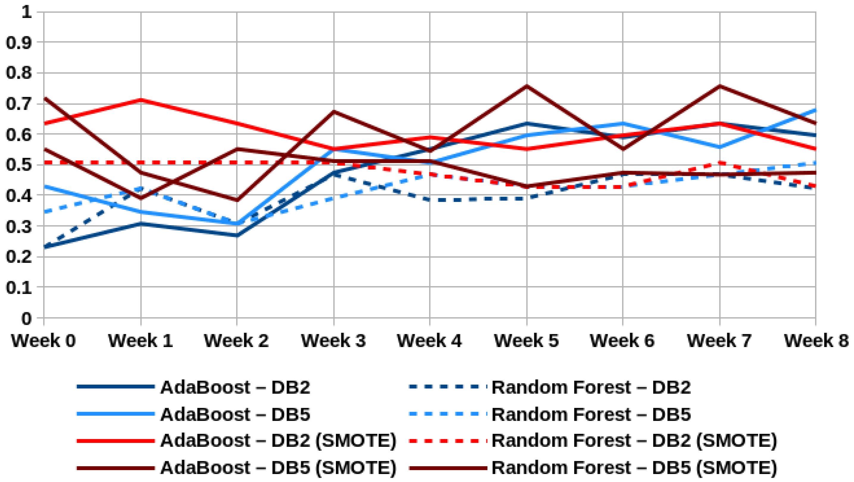
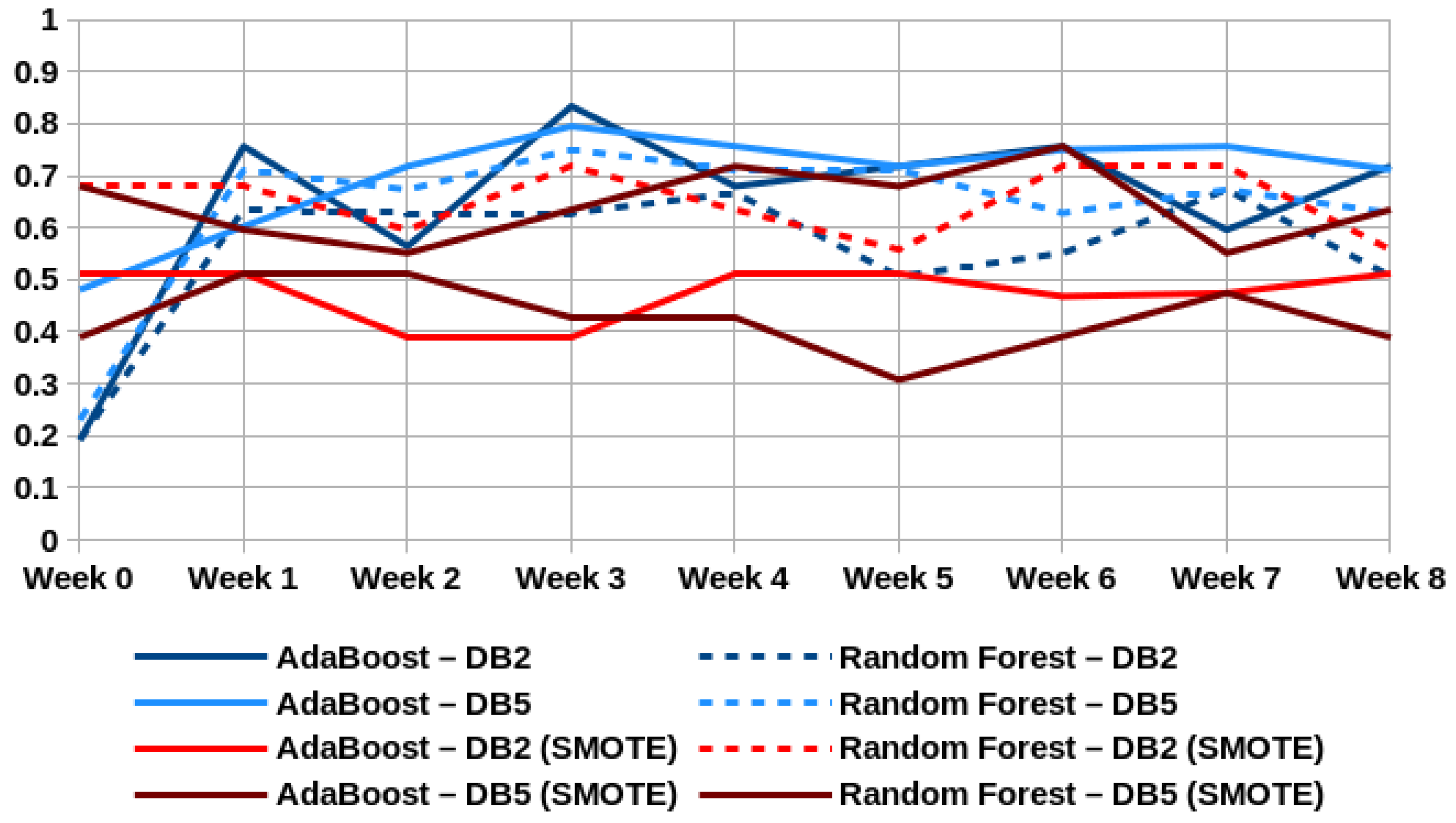
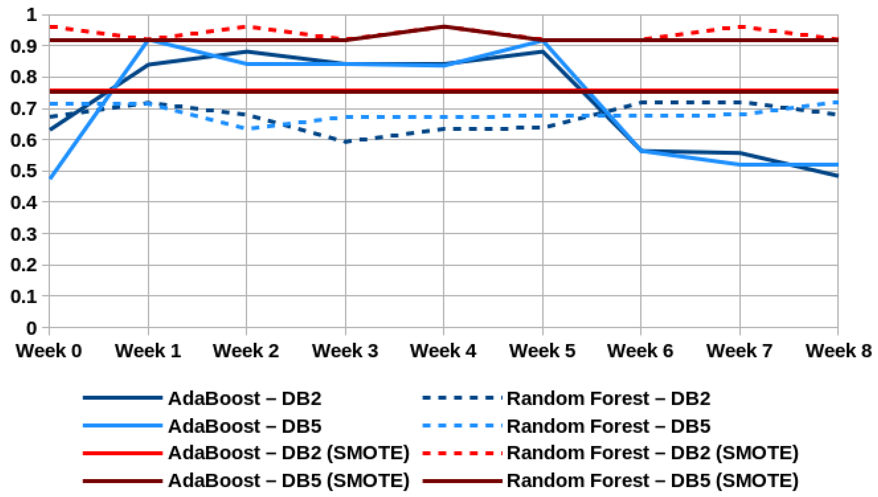
Figure 4, Figure 5, Figure 6 and Figure 7 help to better visualize the results for the first 8 weeks of the four evaluated semesters (2016-1, 2016-2, 2017-1 and 2017-2 respectively).

Figure 4 and Figure 5 show similar results for the semesters 2016-1 and 2016-2, respectively, which are when SMOTE is not applied, the results are better. It happens for the two cases, in both figures. It can be seen in Figure 4 and Figure 5 that the AdaBoost achieved the best prediction result with DB5.

In 2017-1 (Figure 6), it can be seen that the use of SMOTE improved the prediction results since the AdaBoost—DB5 combination with SMOTE presented the best results for the eight week. However, in Week 8, we can see that the Random Forest—DB5 combination presented similar results.

In Figure 7 we can see that the application of SMOTE brought the biggest difference if compared to the data without SMOTE. The Random Forest classifier (with DB2 and DB5) presented the best results and the application of SMOTE improved the results. However, in Week 8, results of Random Forest (without the SMOTE application) and AdaBoost—DB2/DB5 were pretty similar.

From the results, one can say that the use of SMOTE helps on improving the performances of the models in only 43.75% of the cases considering all four semesters. Moreover, the use of SMOTE showed the best improvement on 2017-2, where the ROC value for Random Forest with DB2 and DB5 stayed above all the other combinations on all the weeks.

4.1.4. RQ4. Does the Use of Data from Questionnaires Applied at the Beginning of the Course Help to Improve Models Performance?

To answer this question, we used the same methodology of the previous question, initially not including the use of SMOTE and then applying the SMOTE.

Table 8. Comparison between the ROC values for the normal data and including questionnaire answers.

Semester	Combination	p-Value	Median (Normal)	Median (Questionnaire)
2016-1	DB2—AdaBoost	0.02081	0.55128	0.67308
	DB5—AdaBoost	0.03846	0.55128	0.62820
	DB2—Random Forest	0.48202	0.42308	0.42308
	DB5—Random Forest	0.19819	0.42949	0.38461
2016-2	DB2—AdaBoost	0.44679	0.71795	0.67949
	DB5—AdaBoost	0.05542	0.71795	0.64103
	DB2—Random Forest	0.26698	0.62820	0.62820
	DB5—Random Forest	0.16124	0.67308	0.66667
2017-1	DB2—AdaBoost	0.00302	0.66013	0.49020
	DB5—AdaBoost	0.01466	0.63072	0.49346
	DB2—Random Forest	0.08310	0.54902	0.44118
	DB5—Random Forest	0.41219	0.52287	0.49673
2017-2	DB2—AdaBoost	0.39453	0.83974	0.79808
	DB5—AdaBoost	0.29755	0.83654	0.75641
	DB2—Random Forest	0.48230	0.67949	0.71154
	DB5—Random Forest	0.50000	0.67628	0.67628

presents the results.

On the one hand, in Table 8 it is possible to see the improvement of the performances (median of ROC values) in only 3 out of 16 cases, where only 2 cases are statistically significant. Both in 2016-1, with DB2 and DB5 with AdaBoost. On the other hand, there are some cases where the inclusion of data from the questionnaire decreases the performances of the models, in which two of them have a statistically significant level. According to these results, we can say that using questionnaire data, without performing feature selection, does not help with the prediction of failing of the students.

We also analyzed the case where over-sampled data was compared with the DBs plus questionnaire data (also over-sampled).

Table 9. Comparison between the ROC values on the normal data with oversample and data with oversampled plus questionnaire.

Semester	Combination	p-Value	Median (Oversample)	Median (Questionnaire Data with Oversample)
2016-1	DB2—AdaBoost	0.06890	0.59615	0.58974
	DB5—AdaBoost	0.21254	0.63461	0.58974
	DB2—Random Forest	0.00376	0.50641	0.50641
	DB5—Random Forest	0.13058	0.47436	0.46795
2016-2	DB2—AdaBoost	0.00506	0.51282	0.34615
	DB5—AdaBoost	0.1488	0.42949	0.39102
	DB2—Random Forest	0.0087	0.67949	0.71795
	DB5—Random Forest	0.03328	0.63461	0.71795
2017-1	DB2—AdaBoost	0.28199	0.54575	0.57189
	DB5—AdaBoost	0.2510	0.51961	0.49346
	DB2—Random Forest	0.0015	0.57516	0.66013
	DB5—Random Forest	0.0533	0.63399	0.60457
2017-2	DB2—AdaBoost	0.0000	0.75641	0.79487
	DB5—AdaBoost	0.0000	0.75320	0.79487
	DB2—Random Forest	0.2260	0.91987	0.95833
	DB5—Random Forest	0.02940	0.91987	0.96154

shows the results.

In Table 9, it is important to point out that the results got better in 8 out of 16 cases. However, in these 8 cases better results, there are statistical differences in six of them. Based on these results, we can reinforce our previous statement that data from the questionnaire does not help to improve the performance of the models (even when the datasets are balanced).

5. Conclusions

This work presented a comparative study aiming to find the best combination between dataset and classification algorithm (using and not using pre-processing algorithms) to early predict at-risk students in introductory programming courses. Thirteen dataset combinations together with five classification algorithms (k-Nearest Neighbor, Multilayer Perceptron, Naive Bayes, AdaBoost and Random Forest) were used in the experiments.

The literature has works that also analyze log data from Moodle for generating predictive models for early identification of at-risk students, though the present work differs from them by providing a categorization of the counting of the logs according to the three elements required for a successful computer-mediated learning experience proposed by Garrison et al. [22], that is, cognitive, social and teaching presences.

We tested to which extent the classification of the counting of the logs into these three dimensions would serve as better datasets for the generation of more accurate predictive models. The main idea was that the different classes of students (Approved versus Reproved) would interact differently in those dimensions of presence and that could help the models to better capture students behavior in the learning settings. However, results have shown that there is no improvement in the performance of the models using those three dimensions: cognitive, social and teaching presences. Because of that, one can assume that the simple counting of interactions can be used to generate predictive models, corroborating with previous work [59]. This contradicts the findings of other authors, such as Conijn et al. [37] that say that predictive models cannot be generalized only by the LMS data logs and additional data sources are needed.

Considering that our interest is to early predict at-risk students, we measured the performances of the models until the middle of the semester (8 weeks). It is possible to say that the models achieved performances that can be considered satisfactory (with AUC ROC values of 90% already in the first week) and it is similar to the results found in the literature, for example, Detoni et al. [25], Howard et al. [46], Sandoval et al. [31], and Lu et al. [47]. These results were found considering the pre-processing of the datasets using SMOTE to balance the classes. Even with datasets being highly unbalanced, the use of SMOTE did not helped on increasing the performance of the models, improving on only 43.75% of the cases. Improvements in the performances of the models to predict at-risk students by applying SMOTE were reported in the literature in Costa et al. [24].

At last, we tested whether the inclusion of general, demographic and motivational information about the students would help to increase the performances of the models. The results show that data coming from the questionnaire did not help to improve the performance, contradicting results of other experiments reported by Tillmann et al. [28] and Adejo and Connolly [39], but corroborating previous findings of Brooks et al. [60].

The performance of the models varied according to the semester and the machine learning algorithm in use. The decision of which model apply and the the best moment for that would depend on the specifics of the semester. For instance, in some cases, it is possible to observe a drop in the performance of the models for some algorithms as the semester approaches to the middle. This is the case, for instance, of Adaboost-DB2 and Adaboost-DB5 at week 5 of semester 2017.2 (e.g., see Figure 7. In this scenario, it is recommended to use models generated by Random Forest with the use of SMOTE). From the figures, one could say that the best moment for predicting with good performances and before any significant loss, would be week 3. Again, for each semester, a given set of configuration should be picked accordingly.

One of the main contributions of our work is the investigation of the effectiveness of EDM techniques to early detect at-risk students and the extensive comparison of different combinations of classifiers and dataset (five classification algorithms with 13 DBs, generating 65 combinations for each semester). We also investigated the effect of pre-processing algorithms, such as SMOTE and the use of questionnaire data.

Regarding the courses’ context, activities, tests and assignment, an important discussion that we can provide are about the activities and materials the lecturer provided during the 4 semesters presented in this work. The lecturer gradually improved the quality and the quantity of the resources of the course. It includes VPL exercises, which increased from 53 in 2016-1 to 86 in 2017-2. It also increased the number of other resources (slides, websites, examples, tutorials and so on) from 23 to 60 at the end of 2017-2. A deep analysis of these aspects shows that after the 4th week, students are autonomous to interact with the course’s resources, more specifically, they can start programming using VPL. There are a lot of interactions in Moodle within VPL exercises. It seems that the course structure of the 2017-2 version is more intuitive to the students and it let them interact more precisely with the resources. We are able to conclude that a more structured course, with dozens of materials, best fits the students’ needs, because they can have good interactions with the course and, consequently, succeed. It also seems that student interaction means engagement, and more engagement leads students to succeed.

The limitation of the work lies on the small number of cases included in each dataset (semester), although this limitation was softened with the use of leave-one-out validation during the training and testing of the models and with the use of SMOTE (that generates and includes new synthetic cases in the samples).

Future works include the test of more pre-processing techniques, aiming to improve the quality of the data, since the number of samples used in this work was small. Also, we intend to use other classification algorithms or even a combination of them. Deep Learning techniques can be also used for classification. When available, we intend to process data from 2018 and 2019 to check if there are any differences in the results.

References

1. Bennedsen, J.; Caspersen, M.E. Failure rates in introductory programming: 12 years later. ACM Inroads 2019, 10, 30–36. [Google Scholar] [CrossRef] [Green Version]
2. Watson, C.; Li, F.W. Failure rates in introductory programming revisited. In Proceedings of the 2014 Conference on Innovation & Technology in Computer Science Education, Uppsala, Sweden, 21–25 June 2014; pp. 39–44. [Google Scholar]
3. Dasuki, S.; Quaye, A. Undergraduate Students’ Failure in Programming Courses in Institutions of Higher Education in Developing Countries: A Nigerian Perspective. Electron. J. Inf. Syst. Dev. Ctries. 2016, 76, 1–18. [Google Scholar] [CrossRef] [Green Version]
4. Hawi, N. Causal attributions of success and failure made by undergraduate students in an introductory-level computer programming course. Comput. Educ. 2010, 54, 1127–1136. [Google Scholar] [CrossRef]
5. Krpan, D.; Mladenović, S.; Rosić, M. Undergraduate Programming Courses, Students’ Perception and Success. Procedia- Behav. Sci. 2015, 174, 3868–3872. [Google Scholar] [CrossRef] [Green Version]
6. Jenkins, T. On the difficulty of learning to program. In Proceedings of the 3rd Annual Conference of the LTSN Centre for Information and Computer Sciences, The Higher Education Academy, Loughborough, UK, 27–29 August 2002; Volume 4, pp. 53–58. [Google Scholar]
7. Dunican, E. Making the analogy: Alternative delivery techniques for first year programming courses. In Proceedings of the 14th Workshop of the Psychology of Programming Interest Group, London, UK, 18 June 2002. [Google Scholar]
8. Byrne, P.; Lyons, G. The effect of student attributes on success in programming. Acm Sigcse Bull. 2001, 33, 49–52. [Google Scholar] [CrossRef]
9. BRASSCOM. Relatório Setorial de TIC. Technical Report, Brasscom, 2019. Available online: https://brasscom.org.br/relatorio-setorial-de-tic-2019/ (accessed on 3 October 2019).
10. Gareis, K.; Hüsing, T.; Birov, S.; Bludova, I.; Schulz, C.; Korte, W. E-Skills for Jobs in Europe: Measuring Progress and Moving Ahead; European Commission: Brussels, Belgium, 2014.
11. Korte, W.; Hüsing, T.; Dashja, E. High-Tech Leadership Skills for Europe-Towards an Agenda for 2020 and Beyond; European Communities: Brussels, Belgium, 2017. [Google Scholar]
12. European Political Strategy Centre (EPSC). Global Trends to 2030: The Future of Work and Workspaces. Technical Report, European Strategy and Policy Analysis System, 2018. Available online: https://espas.secure.europarl.europa.eu/orbis/sites/default/files/generated/document/en/Ideas%20Paper%20Future%20of%20work%20V02.pdf (accessed on 3 October 2019).
13. Bughin, J.; Hazan, E.; Lund, S.; Dahlström, P.; Wiesinger, A.; Subramaniam, A. Skill Shift: Automation and the Future of the Workforce; McKinsey Global Institute. McKinsey & Company: Brussels, Belgium, 2018. [Google Scholar]
14. Resnick, M. Mother’s Day, Warrior Cats, and Digital Fluency: Stories from the Scratch Online Community. In Proceedings of the Constructionism 2012 Conference: Theory, Practice and Impact, Athens, Greece, 21–25 August 2012; pp. 52–58. [Google Scholar]
15. Macfadyen, L.P.; Dawson, S. Mining LMS data to develop an ’early warning system’ for educators: A proof of concept. Comput. Educ. 2010, 54, 588–599. [Google Scholar] [CrossRef]
16. Lakkaraju, H.; Aguiar, E.; Shan, C.; Miller, D.; Bhanpuri, N.; Ghani, R.; Addison, K.L. A machine learning framework to identify students at risk of adverse academic outcomes. In Proceedings of the 21th ACM SIGKDD International Conference on Knowledge Discovery and Data Mining, Sydney, NSW, Australia, 10–13 August 2015; pp. 1909–1918. [Google Scholar]
17. Romero, C.; Ventura, S. Data mining in education. Wiley Interdiscip. Rev. Data Min. Knowl. Discov. 2013, 3, 12–27. [Google Scholar] [CrossRef]
18. Mishra, T.; Kumar, D.; Gupta, S. Mining students’ data for prediction performance. In Proceedings of the 2014 Fourth International Conference on Advanced Computing & Communication Technologies (ACCT), Rohtak, India, 8–9 February 2014; pp. 255–262. [Google Scholar]
19. Murray, M.; Pérez, J.; Geist, D.; Hedrick, A. Student interaction with content in online and hybrid courses: Leading horses to the proverbial water. In Proceedings of the Informing Science and Information Technology Education Conference, Porto, Portugal, 1–6 July 2013; Informing Science Institute: Porto, Portugal, 2013; pp. 99–115. [Google Scholar]
20. Dickson, W.P. Toward a Deeper Understanding of Student Performance in Virtual High School Courses: Using qUantitative Analyses and Data Visualization to Inform Decision Making; Technical Report; NCREL/Learning Point Associates: Naperville, IL, USA, 2005; Available online: https://msu.edu/user/pdickson/talks/DicksonNCREL2005.pdf (accessed on 13 December 2019).
21. Romero, C.; Ventura, S. Educational data mining: A review of the state of the art. IEEE Trans. Syst. Man Cybern. Part C Appl. Rev. 2010, 40, 601–618. [Google Scholar] [CrossRef]
22. Garrison, D.R.; Anderson, T.; Archer, W. Critical inquiry in a text-based environment: Computer conferencing in higher education. Internet High. Educ. 1999, 2, 87–105. [Google Scholar] [CrossRef] [Green Version]
23. Swan, K. Learning effectiveness online: What the research tells us. Elem. Qual. Online Educ. Pract. Dir. 2003, 4, 13–47. [Google Scholar]
24. Costa, E.B.; Fonseca, B.; Santana, M.A.; de Araújo, F.F.; Rego, J. Evaluating the effectiveness of educational data mining techniques for early prediction of students’ academic failure in introductory programming courses. Comput. Hum. Behav. 2017, 73, 247–256. [Google Scholar] [CrossRef]
25. Detoni, D.; Cechinel, C.; Matsumura, R.A.; Brauner, D.F. Learning to Identify At-Risk Students in Distance Education Using Interaction Counts. Rev. De Informática Teórica E Apl. 2016, 23, 124–140. [Google Scholar] [CrossRef] [Green Version]
26. Azcona, D.; Hsiao, I.H.; Smeaton, A.F. Detecting students-at-risk in computer programming classes with learning analytics from students’ digital footprints. In User Modeling and User-Adapted Interaction; Springer: Berlin, Germany, 2019; pp. 1–30. [Google Scholar]
27. Leppänen, L.; Leinonen, J.; Ihantola, P.; Hellas, A. Predicting Academic Success Based on Learning Material Usage. In Proceedings of the 18th Annual Conference on Information Technology Education, Rochester, NY, USA, 4–7 October 2017; pp. 13–18. [Google Scholar]
28. Tillmann, A.; Krömker, D.; Horn, F.; Gattinger, T. Analysing & Predicting Students Performance in an Introductory Computer Science Course; Hochschuldidaktik der Informatik HDI 2018; Universität Potsdam: Potsdam, Germany, 2018; pp. 29–46. [Google Scholar]
29. Sheshadri, A.; Gitinabard, N.; Lynch, C.F.; Barnes, T.; Heckman, S. Predicting student performance based on online study habits: A study of blended courses. arXiv 2019, arXiv:1904.07331. [Google Scholar]
30. Jokhan, A.; Sharma, B.; Singh, S. Early warning system as a predictor for student performance in higher education blended courses. Stud. Higher Educ. 2018, 44, 1900–1911. [Google Scholar] [CrossRef]
31. Sandoval, A.; Gonzalez, C.; Alarcon, R.; Pichara, K.; Montenegro, M. Centralized student performance prediction in large courses based on low-cost variables in an institutional context. Internet High. Educ. 2018, 37, 76–89. [Google Scholar] [CrossRef]
32. Mwalumbwe, I.; Mtebe, J.S. Using learning analytics to predict students’ performance in moodle learning management system: A case of mbeya university of science and technology. Electron. J. Inf. Syst. Dev. Ctries. 2017, 79, 1–13. [Google Scholar] [CrossRef] [Green Version]
33. Hung, J.L.; Wang, M.C.; Wang, S.; Abdelrasoul, M.; Li, Y.; He, W. Identifying at-risk students for early interventions—A time-series clustering approach. IEEE Trans. Emerg. Top. Comput. 2017, 5, 45–55. [Google Scholar] [CrossRef]
34. Soffer, T.; Cohen, A. Students’ engagement characteristics predict success and completion of online courses. J. Comput. Assisted Learn. 2019, 35, 378–389. [Google Scholar] [CrossRef]
35. Kostopoulos, G.; Kotsiantis, S.; Pierrakeas, C.; Koutsonikos, G.; Gravvanis, G.A. Forecasting students’ success in an open university. Int. J. Learn. Technol. 2018, 13, 26–43. [Google Scholar] [CrossRef]
36. Baneres, D.; Rodriguez-Gonzalez, M.E.; Serra, M. An Early Feedback Prediction System for Learners At-risk within a First-year Higher Education Course. IEEE Trans. Learn. Technol. 2019, 12, 249–263. [Google Scholar] [CrossRef]
37. Conijn, R.; Snijders, C.; Kleingeld, A.; Matzat, U. Predicting student performance from LMS data: A comparison of 17 blended courses using Moodle. IEEE Trans. Learn. Technol. 2017, 10, 17–29. [Google Scholar] [CrossRef]
38. Sukhbaatar, O.; Ogata, K.; Usagawa, T. Mining Educational Data to Predict Academic Dropouts: A Case Study in Blended Learning Course. In Proceedings of the IEEE TENCON 2018-2018 IEEE Region 10 Conference, Jeju, Korea, 28–31 October 2018; pp. 2205–2208. [Google Scholar]
39. Adejo, O.W.; Connolly, T. Predicting student academic performance using multi-model heterogeneous ensemble approach. J. Appl. Res. High. Educ. 2018, 10, 61–75. [Google Scholar] [CrossRef]
40. Umer, R.; Mathrani, A.; Susnjak, T.; Lim, S. Mining Activity Log Data to Predict Student’s Outcome in a Course. In Proceedings of the 2019 International Conference on Big Data and Education, London, UK, 30 March–1 April 2019; pp. 52–58. [Google Scholar]
41. Olivé, D.M.; Huynh, D.; Reynolds, M.; Dougiamas, M.; Wiese, D. A Quest for a one-size-fits-all Neural Network: Early Prediction of Students At Risk in Online Courses. IEEE Trans. Learn. Technol. 2019, 12, 171–183. [Google Scholar] [CrossRef]
42. Cohen, A. Analysis of student activity in web-supported courses as a tool for predicting dropout. Educ. Technol. Res. Dev. 2017, 65, 1285–1304. [Google Scholar] [CrossRef]
43. Kondo, N.; Okubo, M.; Hatanaka, T. Early Detection of At-Risk Students Using Machine Learning Based on LMS Log Data. In Proceedings of the 2017 6th IIAI International Congress on Advanced Applied Informatics (IIAI-AAI), Hamamatsu, Japan, 9–13 July 2017; pp. 198–201. [Google Scholar]
44. Usman, U.I.; Salisu, A.; Barroon, A.I.; Yusuf, A. A Comparative Study of Base Classifiers in Predicting Students’ Performance based on Interaction with LMS Platform. FUDMA J. Sci. 2019, 3, 231–239. [Google Scholar]
45. Zhou, Q.; Quan, W.; Zhong, Y.; Xiao, W.; Mou, C.; Wang, Y. Predicting high-risk students using Internet access logs. Knowl. Inf. Syst. 2018, 55, 393–413. [Google Scholar] [CrossRef]
46. Howard, E.; Meehan, M.; Parnell, A. Contrasting prediction methods for early warning systems at undergraduate level. Internet High. Educ. 2018, 37, 66–75. [Google Scholar] [CrossRef] [Green Version]
47. Lu, O.H.; Huang, A.Y.; Huang, J.C.; Lin, A.J.; Ogata, H.; Yang, S.J. Applying Learning Analytics for the Early Prediction of Students’ Academic Performance in Blended Learning. J. Educ. Technol. Soc. 2018, 21, 220–232. [Google Scholar]
48. Gray, C.C.; Perkins, D. Utilizing early engagement and machine learning to predict student outcomes. Comput. Educ. 2019, 131, 22–32. [Google Scholar] [CrossRef]
49. Rodríguez-del Pino, J.C.; Rubio-Royo, E.; Hernández-Figueroa, Z.J. A Virtual Programming Lab for Moodle with automatic assessment and anti-plagiarism features. In Proceedings of the International Conference on e-Learning, e-Business, Enterprise Information Systems, and e-Government (EEE), Las Vegas, ND, USA, 16–19 July 2012; The Steering Committee of The World Congress in Computer Science, CSREA Press: Las Vegas, ND, USA, 2012; pp. 80–85. [Google Scholar]
50. Detoni, D.; Cechinel, C.; Matsumura Araújo, R. Modelagem e Predição de Reprovação de Acadêmicos de Cursos de Educação a Distância a partir da Contagem de Interações. Revista Brasileira de Informática na Educação 2015, 23, 1–11. [Google Scholar]
51. Moore, M.G. Three types of interaction. Am. J. Distance Educ. 1989, 3, 1–7. [Google Scholar]
52. McKinney, W. Data structures for statistical computing in python. In Proceedings of the 9th Python in Science Conference, Austin, TX, USA, 28–30 June 2010; Volume 445, pp. 51–56. [Google Scholar]
53. Chawla, N.V.; Bowyer, K.W.; Hall, L.O.; Kegelmeyer, W.P. SMOTE: Synthetic minority over-sampling technique. J. Artif. Intell. Res. 2002, 16, 321–357. [Google Scholar] [CrossRef]
54. Lemaître, G.; Nogueira, F.; Aridas, C.K. Imbalanced-learn: A Python Toolbox to Tackle the Curse of Imbalanced Datasets in Machine Learning. J. Mach. Learn. Res. 2017, 18, 1–5. [Google Scholar]
55. Pedregosa, F.; Varoquaux, G.; Gramfort, A.; Michel, V.; Thirion, B.; Grisel, O.; Blondel, M.; Prettenhofer, P.; Weiss, R.; Dubourg, V.; et al. Scikit-learn: Machine Learning in Python. J. Mach. Learn. Res. 2011, 12, 2825–2830. [Google Scholar]
56. Bradley, A.P. The use of the area under the ROC curve in the evaluation of machine learning algorithms. Pattern Recognit. 1997, 30, 1145–1159. [Google Scholar] [CrossRef] [Green Version]
57. Gašević, D.; Dawson, S.; Rogers, T.; Gasevic, D. Learning analytics should not promote one size fits all: The effects of instructional conditions in predicting academic success. Internet High. Educ. 2016, 28, 68–84. [Google Scholar] [CrossRef] [Green Version]
58. Mann, H.B.; Whitney, D.R. On a test of whether one of two random variables is stochastically larger than the other. Ann. Math. Stat. 1947, 18, 50–60. [Google Scholar] [CrossRef]
59. Umer, R.; Susnjak, T.; Mathrani, A.; Suriadi, S. A learning analytics approach: Using online weekly student engagement data to make predictions on student performance. In Proceedings of the 2018 International Conference on Computing, Electronic and Electrical Engineering (ICE Cube), Quetta, Pakistan, 12–13 November 2018; pp. 1–5. [Google Scholar]
60. Brooks, C.; Thompson, C.; Teasley, S. Who you are or what you do: Comparing the predictive power of demographics vs. activity patterns in massive open online courses (MOOCs). In Proceedings of the Second (2015) ACM Conference on Learning@ Scale, Vancouver, BC, Canada, 14–18 March 2015; pp. 245–248. [Google Scholar]
Figure 1. Overview of the adopted methodology.
Applsci 09 05523 g001
Figure 2. Steps of the adopted methodology. The “Pre-Processing” step was showed in dotted lines because it is optional, i.e., applied only in some experiments.
Applsci 09 05523 g002
Figure 3. Interaction frequency distribution in each week for every semester.
Applsci 09 05523 g003
Figure 4. ROC Curve: 2016-1.
Applsci 09 05523 g004
Figure 5. ROC Curve: 2016-2.
Applsci 09 05523 g005
Figure 6. ROC Curve: 2017-1.
Applsci 09 05523 g006
Figure 7. ROC Curve: 2017-2.
Applsci 09 05523 g007