Adaptive Threshold-Aided K-Best Sphere Decoding for Large MIMO Systems

Abstract

This paper proposes an adaptive threshold-aided K-best sphere decoding (AKSD) algorithm for large multiple-input multiple-output systems. In the proposed scheme, to reduce the average number of visited nodes compared to the conventional K-best sphere decoding (KSD), the threshold for retaining the nodes is adaptively determined at each layer of the tree. Specifically, we calculate the adaptive threshold based on the signal-to-noise ratio and index of the layer. The ratio between the first and second smallest accumulated path metrics at each layer is also exploited to determine the threshold value. In each layer, in addition to the K paths associated with the smallest path metrics, we also retain the paths whose path metrics are within the threshold from the Kth smallest path metric. The simulation results show that the proposed AKSD provides nearly the same bit error rate performance as the conventional KSD scheme while achieving a significant reduction in the average number of visited nodes, especially at high signal-to-noise ratios.

1. Introduction

Large multiple-input multiple-output (MIMO) systems have received enormous attention from researchers in the field of wireless communication for their high spectral and power efficiency [1]. However, the promised benefits of large MIMO are expensive in terms of computational complexity at the receiver compared to the conventional MIMO systems [1,2]. In conventional MIMO systems, to simplify the exhaustive search of the optimal maximum likelihood (ML) receiver, a sphere decoder (SD) can be employed, which only searches for the ML solution inside a sphere to reduce computational complexity. Furthermore, low-complexity sub-optimal algorithms including parallel interference cancellation (PIC) [3] and successive interference cancellation (SIC) [4] can also be considered. However, to approach the channel capacity, it is required to employ a near-optimal receiver such as the SD. Even though the SD performs close to the ML receiver, its complexity grows exponentially with the number of transmit antennas, which results in excessively large complexity in large MIMO systems [2,5].

Among variants of SD, K-best SD (KSD) begins its search from the first layer, and K candidate paths that are associated with the smallest path metrics at each layer are preserved for the subsequent layers until the iteration process reaches the leaf layer [6,7]. Then, the one with the smallest path metric is chosen as the hard decision output of the KSD algorithm. The KSD requires fixed detection complexity [7] and can be implemented in a parallel fashion, which makes it suitable for hardware implementation [8]. However, to approach the bit-error rate (BER) performance of the original SD, the KSD needs to retain a large number of nodes in each layer, as presented in [9], which leads to a large computational complexity.

This paper presents an adaptive threshold-aided K-best SD (AKSD) algorithm. Unlike the traditional KSD, where the number of survival nodes is constant, in AKSD, the number of retained nodes dynamically changes in each layer of the tree. Specifically, to reduce the complexity while maintaining the near-optimal BER performance, we keep the nodes whose path metric is smaller than the Kth node’s metric plus threshold ${\mathsf{\Delta }}_i$. At each layer, the threshold is updated dynamically based on the signal-to-noise ratio (SNR) and the index of the tree-search layer. Furthermore, the ratio between the first and second smallest path metrics is also employed to determine the threshold. Intuitively, if the first minimum path metric is far less than the second, the path associated with the first is very likely to be an ML solution. Therefore, there is no need to keep a large number of nodes. In contrast, if this ratio is small, which decreases the probability that the path with the minimum path metric is the ML solution, then we need to keep a large number of nodes. The main contributions of this study can be summarized as follows:

• We propose the AKSD algorithm, in which the adaptive threshold controls the number of visited nodes in each layer of the tree. In this algorithm, the threshold for retaining the most promising nodes at each layer is adaptively determined based on the ratio between the first and second minimum path metrics at each layer, the SNR, and the layer index.
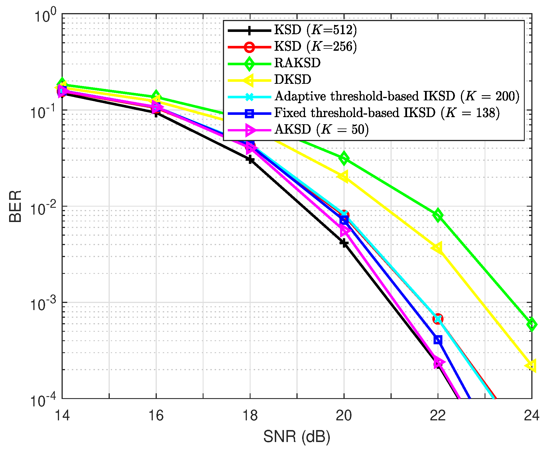
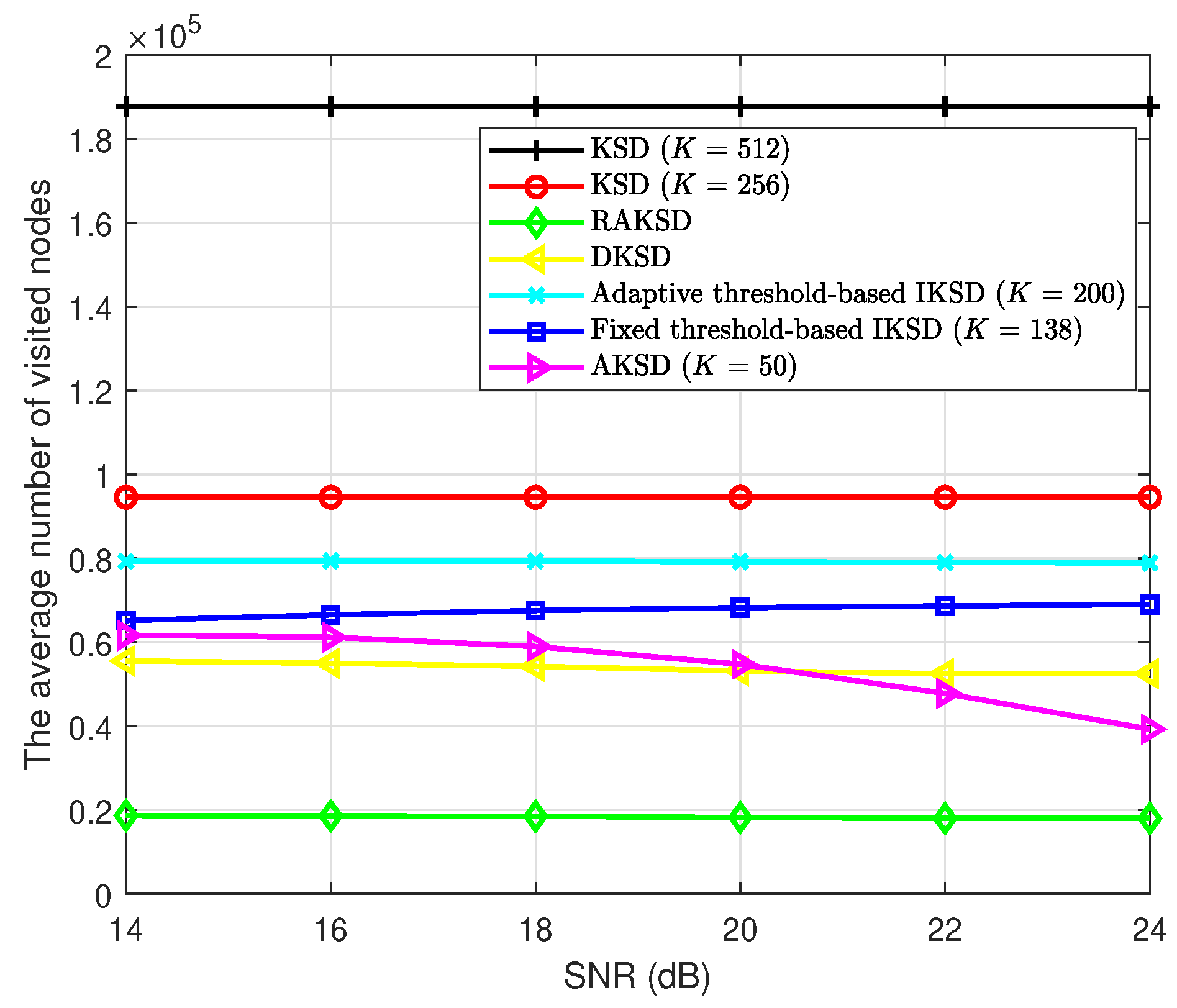
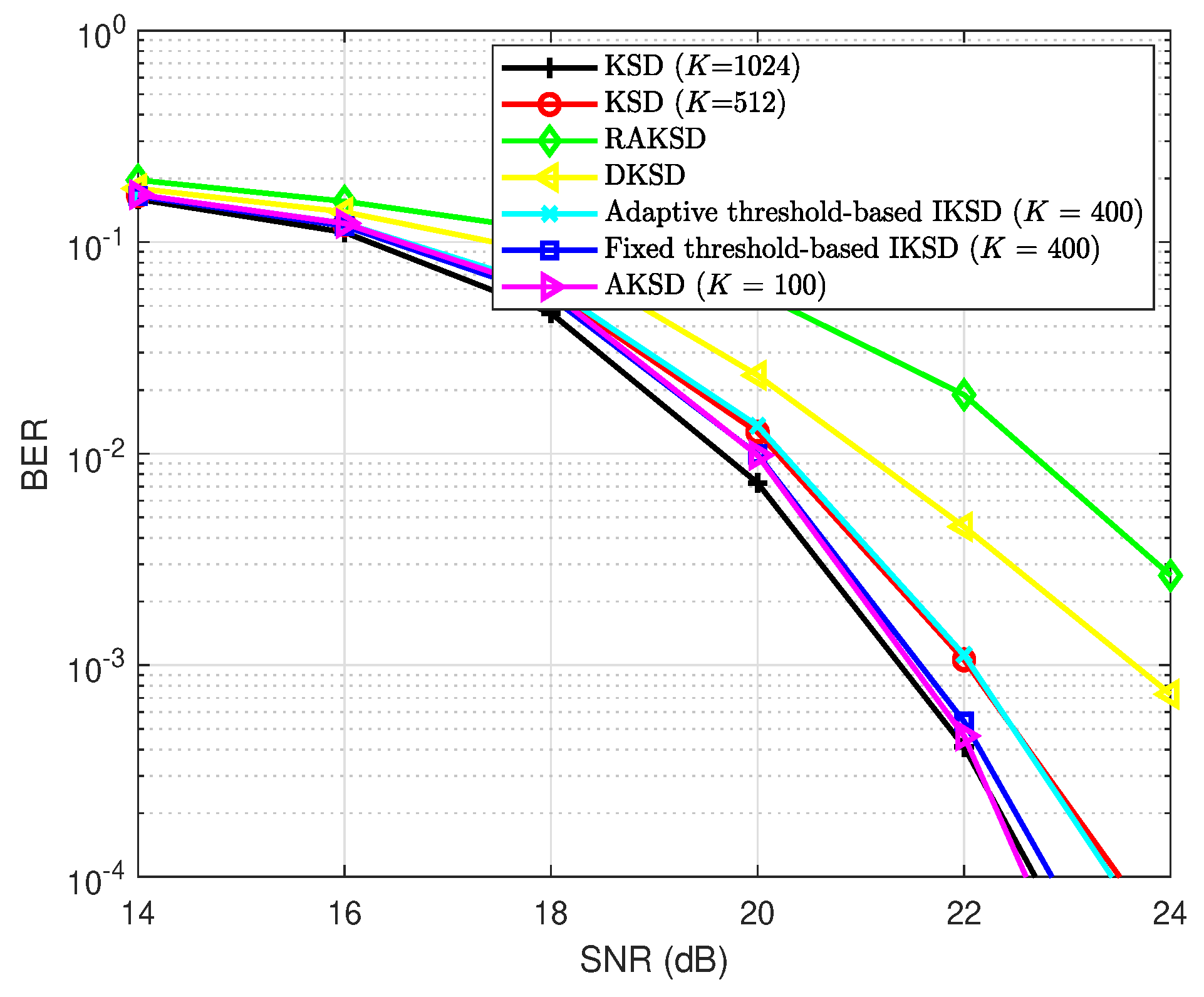
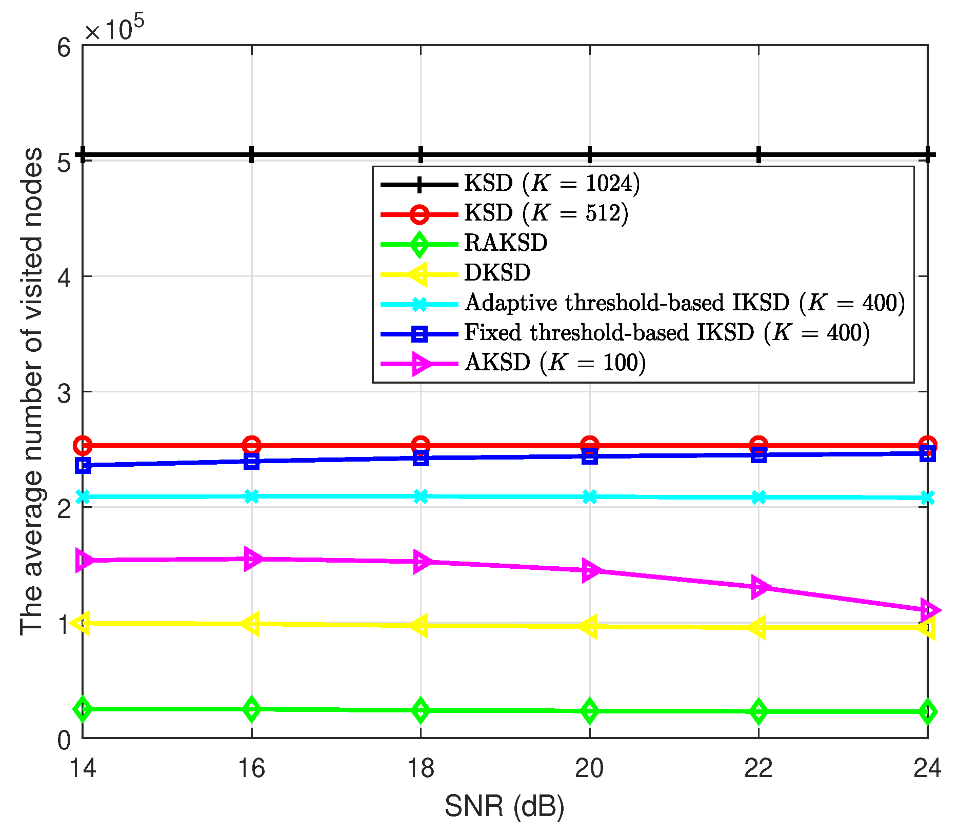
• To evaluate the performance of the proposed AKSD algorithm, we have performed simulations for large MIMO systems. The simulation results show that, compared to the conventional KSD algorithm, the AKSD algorithm requires up to 71% less computational complexity.

The rest of this paper is organized as follows. Section 2 describes the MIMO system model and the conventional SD algorithm. Section 3 explains the traditional KSD and proposed AKSD algorithm. The simulation results and discussions with respect to the BER performance and computational complexity are presented in Section 4. Finally, the conclusions of the study are described in Section 5.

Notations: A boldface capital letter, $\mathbf{X}$, is used to denote a matrix, and a boldface lowercase letter, $\mathbf{x}$, represents a column vector. The nth row and mth column entry of $\mathbf{X}$ is denoted by $x_{n,m}$, whereas the nth entry of vector $\mathbf{x}$ is denoted by $x_n$. The transpose operation is denoted by ${(·)}^T$, and the norm of a vector is denoted by $∥·∥$. Furthermore, $\Re (·)$ and $\Im (·)$ indicate the real and imaginary parts of a matrix or vector, respectively.

2. Background

2.1. MIMO System Description

In a MIMO system with $N_t$ transmit and $M_r$ receive antennas, the received signal vector $\tilde{\mathbf{y}}={[{\tilde{y}}_1,{\tilde{y}}_2,\dots ,{\tilde{y}}_{N_r}]}^T$ is given by

$$\tilde{\mathbf{y}}=\tilde{\mathbf{H}}{\tilde{\mathbf{s}}}_t+\tilde{\mathbf{n}},$$

(1)

where ${\tilde{\mathbf{s}}}_t={[{\tilde{s}}_{t,1},{\tilde{s}}_{t,2},\dots ,{\tilde{s}}_{t,N_t}]}^T$ is the transmitted signal vector with each component independently drawn from a complex constellation, such as quadrature amplitude modulation (QAM), and $\tilde{\mathbf{H}}$ denotes an $N_r\times N_t$ channel matrix, where ${\tilde{h}}_{i,j}$ is the complex channel gain between the jth transmit antenna and ith receive antenna. Furthermore, $\tilde{\mathbf{n}}={\left[{\tilde{n}}_1,{\tilde{n}}_2,\cdots {\tilde{n}}_{N_r}\right]}^T$ is a noise vector consisting of independent and identically distributed additive white Gaussian noise (AWGN) samples with zero mean and unit variance. We assume that the channel matrix is perfectly known at the receiver.

Complex system model (1) can be transformed to its equivalent real signal model $\mathbf{y}=\mathbf{H}{\mathbf{s}}_t+\mathbf{n}$, i.e.,

$$\left[\begin{array}{c}\Re \left(\tilde{\mathbf{y}}\right)\\ \Im \left(\tilde{\mathbf{y}}\right)\end{array}\right]=\left[\begin{array}{cc}\Re \left(\tilde{\mathbf{H}}\right)& -\Im \left(\tilde{\mathbf{H}}\right)\\ \Im \left(\tilde{\mathbf{H}}\right)& \Re \left(\tilde{\mathbf{H}}\right)\end{array}\right]\left[\begin{array}{c}\Re \left({\tilde{\mathbf{s}}}_t\right)\\ \Im \left({\tilde{\mathbf{s}}}_t\right)\end{array}\right]+\left[\begin{array}{c}\Re \left(\tilde{\mathbf{n}}\right)\\ \Im \left(\tilde{\mathbf{n}}\right)\end{array}\right].$$

(2)

In (2), the dimension of the matrices and vectors doubles compared to (1), i.e., ${\mathbf{s}}_t$ contains $N=2N_t$ elements, and the $(M\times 1)$-received signal vector $\mathbf{y}$, $(M\times N)$-channel matrix $\mathbf{H}$, and $(M\times 1)$-noise signal vector $\mathbf{n}$ also double their dimensions, such that $M=2N_r$.

Based on signal model (2), the optimal solution ${\widehat{\mathbf{s}}}_{\mathrm{ML}}$ can be determined as

$${\widehat{\mathbf{s}}}_{\mathrm{ML}}=arg\underset{\mathbf{s}\in {\mathsf{\Omega }}^N}{min}{\parallel \mathbf{y}-\mathbf{Hs}\parallel }^2,$$

(3)

where ${∥\mathbf{y}-\mathbf{Hs}∥}^2$ is the ML metric value for $\mathbf{s}$, and $\mathsf{\Omega }$ denotes the set of real entries in the constellation, e.g., $\mathsf{\Omega }=\{-3,-1,1,3\}$ in the case of 16-QAM.

2.2. Sphere Decoder for MIMO

The SD algorithm aims to reduce the complexity of ML detection by searching only inside a sphere [10,11,12]. Taking the QR decomposition of the channel matrix as $\mathbf{H}=\mathbf{QR}$, where Q is an $(M\times N)$ matrix satisfying ${\mathbf{Q}}^T\mathbf{Q}=\mathbf{I}$, and $\mathbf{R}$ is an upper triangular matrix of size $N\times N$, (3) transforms into the minimization of ${\widehat{\mathbf{s}}}_{\mathrm{ML}}={∥\mathbf{z}-\mathbf{R}\mathbf{s}∥}^2$, where $\mathbf{z}={\mathbf{Q}}^T\mathbf{y}$. The SD examines all signal vector candidates inside a sphere to generate the detection output

$${\widehat{\mathbf{s}}}_{\mathrm{SD}}=arg\underset{\mathbf{s}\in D}{min}{\parallel \mathbf{z}-\mathbf{Rs}\parallel }^2,D=\left\{\mathbf{s}\in {\mathsf{\Omega }}^N|{∥\mathbf{z}-\mathbf{Rs}∥}^2\le C_0^2\right\},$$

(4)

where $C_0$ denotes the initial radius of the sphere. At layer i of the SD, we use the condition

$$|z_i-\sum _{j=i}^N{r}_{i,j}{s}_j{|}^2\le d,d=C_0^2-T\left({\mathbf{s}}^{(i+1)}\right)$$

(5)

to determine a set of surviving paths $\left\{{\mathbf{s}}^{\left(i\right)}\right\}$, where ${\mathbf{s}}^{\left(i\right)}={[s_i^{\left(i\right)},s_{i+1}^{\left(i\right)},\cdots ,s_N^{\left(i\right)}]}^T$ is a surviving path at layer i, and $T\left({\mathbf{s}}^{\left(i\right)}\right)$ is the accumulated path metric of ${\mathbf{s}}^{\left(i\right)}$, which is defined as

$$T\left({\mathbf{s}}^{\left(i\right)}\right)=\sum _{k=i}^N|z_k-\sum _{j=k}^N{r}_{k,j}{s}_j^{\left(i\right)}{|}^2.$$

(6)

In this work, the initial radius is chosen as $C_0=\sqrt{\gamma N{\sigma }^2}$, where $\gamma ⩾1$ is typically set to nearly guarantee that the true solution exits in the sphere [8]. The radius is updated when the search process reaches the leaf layer [13]. The iterative search of SD continues until only one point is left inside the sphere and is a solution to (4).

3. K-Best SD Algorithm

3.1. Conventional KSD Algorithm

Tree-search algorithms are categorized as depth-first and breadth-first search methods [8]. In the typical KSD algorithm, the tree is traversed in a breadth-first fashion, and the search proceeds in the forward direction by keeping only the K best nodes at each layer of the tree [8]. Because of the breadth-first search method, the KSD algorithm does not update the sphere radius [9]. The search process starts from the root node ($i=N$), which represents the Nth transmitted symbol, and proceeds down to the leaf layer $(i=1)$. At the Nth layer, K nodes with the smallest path metrics are kept to extend to the next layer, and the other nodes are pruned.

Each of the K retained parent nodes is extended to its $\left|\mathsf{\Omega }\right|$ children nodes. Therefore, in the $(N-1)$th layer, the number of contender paths becomes $K\left|\mathsf{\Omega }\right|$, and, again, only K paths associated with the smallest path metrics at the $(N-1)$th layer are selected as parent nodes to the next layer. Specifically, we sort the candidate paths in ascending order of their path metrics $T\left({\mathbf{s}}^{\left(i\right)}\right)$ in (6). Let $\left\{{\tau }_i^{\left(l\right)}\right\}$ denote the ordered path metrics of $T\left({\mathbf{s}}^{\left(i\right)}\right)$, where $l=1,2,\cdots ,K\left|\mathsf{\Omega }\right|$. For example, ${\tau }_i^{\left(K\right)}$ is the Kth smallest path metric for the surviving paths at the ith layer. Then, the paths associated with ${\tau }_i^{\left(1\right)},{\tau }_i^{\left(2\right)},\dots ,{\tau }_i^{\left(K\right)}$ are retained, whereas the other paths are pruned.

The search process continues until it reaches the leaf layer. At the leaf layer, each path corresponds to a candidate of the transmitted signal vector, and the one with the minimum path metric among K contender paths is chosen as the final solution.

3.2. Adaptive Threshold for KSD

To reduce the computational complexity of the KSD, which can eventually lead to an improved trade-off between the complexity and performance, we consider dynamically adjusting the number of retained nodes at each layer rather than retaining a fixed number of nodes.

In the AKSD scheme, the number of retained nodes at each layer is adaptively determined. Specifically, in AKSD, we first select K contender paths associated with the K smallest path metrics at each layer of the tree. In addition to those K paths, we choose additional paths whose path metric is close to that of the Kth path, ${\tau }_i^{\left(K\right)}$, within a threshold ${\mathsf{\Delta }}_i$. Specifically, if the difference between ${\tau }_i^{(K+m)}$ and ${\tau }_i^{\left(K\right)}$ is less than ${\mathsf{\Delta }}_i$, i.e.,

$${\tau }_i^{(K+m)}\le {\mathsf{\Delta }}_i+{\tau }_i^{\left(K\right)},$$

(7)

the node corresponding to ${\tau }_i^{(K+m)}$ is retained. When only ${\tau }_i^{\left(l\right)}$, $l=1,2,\cdots ,m$, satisfies (7), then $(K+m)$ nodes corresponding to ${\tau }_i^{\left(1\right)},{\tau }_i^{\left(2\right)},\cdots ,{\tau }_i^{(K+m)}$ are retained, whereas those associated with ${\tau }_i^{(m+1)},\cdots ,{\tau }_i^{\left(K\right|\mathsf{\Omega }\left|\right)}$ are discarded.

Let $K_v$ and $K_p$ be the numbers of visited and survival nodes at a layer, respectively. Then, the number of survival nodes becomes $K_p=K+m$ under the assumption that all the survival nodes satisfy the sphere constraint (5). In the $(i-1)$th layer, $K_v$ is updated to $K_v=K_p\left|\mathsf{\Omega }\right|$.

The threshold at layer i is given by

$${\mathsf{\Delta }}_i=\alpha {\displaystyle \frac{i}{\rho \eta }},$$

(8)

where $\alpha$ is a constant value to control the threshold, which can be used to optimize the trade-off between performance and complexity, and $\rho$ is the SNR. Furthermore, $\eta ={\tau }_i^{\left(2\right)}/{\tau }_i^{\left(1\right)}$ is the ratio between the second smallest path metric ${\tau }_i^{\left(2\right)}$ and the smallest path metric ${\tau }_i^{\left(1\right)}$ at the ith layer.

In the low-SNR region, a relatively large number of nodes need to be retained to obtain the optimal solution, whereas a small number of retained nodes can be enough at high SNRs. Therefore, in (8), ${\mathsf{\Delta }}_i$ is chosen to be inversely proportional to $\rho$. Furthermore, to reduce the effect of error propagation, especially in large MIMO systems, where the tree search processes a large number of layers, more nodes should be kept in the higher layers and fewer in the bottom layers. Therefore, ${\mathsf{\Delta }}_i$ is chosen to be proportional to the layer index i, as shown in (8).

Intuitively, as the difference between the paths with the first and second smallest path metrics becomes larger, the path with the first smallest path metric becomes more likely to be the true solution [14]. In other words, the node corresponding to the first minimum path metric could lead to the final optimal solution. Therefore, the threshold ${\mathsf{\Delta }}_i$ decreases with the ratio between ${\tau }_i^{\left(2\right)}$ and ${\tau }_i^{\left(1\right)}$, as shown in (8).

Algorithm 1 summarizes the procedure of the proposed AKSD scheme. In Algorithm 1, steps 1–7 are used to find the path metrics at each layer of the tree. In step 8, the path metrics are ordered to generate $\left\{{\tau }_i^{\left(l\right)}\right\}$. Step 9 computes the threshold ${\mathsf{\Delta }}_i$, which is then used to determine the paths to retain in step 10.

Algorithm 1: The AKSD Algorithm.

INPUT:  $\mathbf{R},\mathbf{z},K,\rho$, $C_0$, $\alpha$ OUTPUT:  $\widehat{\mathbf{s}}$. 1: for$i=N$to 1 do 2:     if $i=N$ then 3:         Calculate the path metric of each path ${\mathbf{s}}^{\left(i\right)}$: 4:         $T\left({\mathbf{s}}^{\left(i\right)}\right)$ = $|z_i-r_{i,i}{s}_i^{\left(i\right)}{|}^2$, $s_i^{\left(i\right)}\in \mathsf{\Omega }$, 5:     else 6:         Expand all the surviving $K_p$ nodes at the ith layer 7:         to all $\left|\mathsf{\Omega }\right|$ children nodes to generate $\left\{{\mathbf{s}}^{\left(i\right)}\right\}$. 8:         For each path ${\mathbf{s}}^{\left(i\right)}$, compute the path metric: 9:         $T\left({\mathbf{s}}^{\left(i\right)}\right)={\sum }_{k=i}^N|z_k-{\sum }_{j=k}^N{r}_{k,j}{s}_j^{\left(i\right)}{|}^2$, 10:     end if 11:     Find ${\tau }_i^{\left(l\right)}$, $l=1,2,\cdots ,K_p\left|\mathsf{\Omega }\right|$, by sorting the elements in $\left\{T\left({\mathbf{s}}^{\left(i\right)}\right)\right\}$ in ascending order. 12:     Calculate ${\mathsf{\Delta }}_i$ in (8). 13:     Keep the K smallest path metric nodes and the nodes satisfying (7) and 14:     the sphere constraint (5), then update $K_p$. 15: end for 16: Set the surviving path with the smallest path metric to output $\widehat{\mathbf{s}}$.

4. Simulation Results

The proposed AKSD and the conventional KSD were tested with various values of K for comparison. The improved K-best SD (IKSD) algorithm [7] was also considered for comparison. In [7], three threshold rules were proposed, namely, the adaptive, normalized, and fixed thresholds. In this study, for comparison, we tested the adaptive threshold-based IKSD and the fixed threshold-based IKSD. In addition, the schemes in [9,14] were tested for comparison. The radius adaptive K-best decoder (RAKSD) in [9] employs tree decomposition and adaptive pruning to reduce the complexity, whereas the dynamic threshold-aided K-best sphere decoder (DKSD) in [14] exploits a dynamic threshold to adjust K. For the threshold in the proposed AKSD algorithm, the constant $\alpha$ was set to 1. For the initial radius, we set $\gamma =5$, as in [8]. The complexity was measured by the average number of visited nodes. Furthermore, the mean values in the simulation results were obtained by averaging over ${10}^7$ independent channel realizations. For simulations, we considered two large MIMO configurations: $(N_r,N_t,$$\mathsf{\Omega })=$$(48,48,16)$ and $(64,64,16)$.

In Figure 1, the BER comparison results for a MIMO system with $N_r=48$, $N_t=48$, and 16-QAM are shown. We can observe that the AKSD scheme with relatively small K achieves comparable or better BER performance with respect to the conventional KSD scheme with large K. Specifically, the performance of the proposed AKSD with $\mathit{K}=50$ is nearly the same as that of the conventional KSD with $\mathit{K}=512$ at high SNRs, where the AKSD achieves an SNR gain of 0.7 dB over the conventional KSD with $\mathit{K}=256$ at BER $={10}^{-4}$. Figure 1 also shows that the AKSD scheme achieves better BER performance compared to the adaptive threshold-based IKSD and fixed threshold-based IKSD. The SNR gains of the AKSD at BER $={10}^{-4}$ over the adaptive threshold-based IKSD with $\mathit{K}=200$ and the fixed threshold-based IKSD with $\mathit{K}=138$ are approximately $0.7$ dB and $0.25$ dB, respectively. Moreover, the AKSD scheme outperforms both the RAKSD and DKSD by approximately $2.0$ dB and $2.5$ dB, respectively, at a BER of ${10}^{-3}$.

Figure 2 compares the BER performance for $N_r=64$, $N_t=64$, and 16-QAM. Similar to Figure 1, it demonstrates that the AKSD scheme achieves nearly the same BER performance with that of the conventional KSD scheme with larger K at high SNRs. It is also worth noting that the proposed AKSD outperforms the fixed threshold-based IKSD with $K=400$, achieving an approximate SNR gain of $0.3$ dB for BER $={10}^{-4}$. In Figure 2, it is also observed that the AKSD scheme substantially outperforms the DKSD and RAKSD schemes.

In Figure 3, the complexity comparison for a MIMO system with $N_r=48,N_t=48$ and 16-QAM is shown. Figure 3 shows that the RAKSD scheme requires lower complexity than the other compared schemes; however, its BER performance is significantly worse than those of the other schemes, as shown in Figure 1. A similar observation can also be made for the DKSD scheme. Figure 3 also shows that the proposed scheme requires lower complexity than the other schemes providing comparable BER performances. Specifically, the complexity-reduction ratio of the AKSD at SNR = 20 dB, compared with the conventional KSD with $\mathit{K}=512$ is approximately $70\%$, whereas they achieve comparable BER performance, as shown in Figure 1. Furthermore, the AKSD scheme provides $20\%$ and $31\%$ complexity savings compared with the fixed threshold-based IKSD and the adaptive threshold-based IKSD, respectively. We note that the AKSD scheme outperforms the fixed threshold-based IKSD and adaptive threshold-based IKSD in terms of BER performance. In Figure 3, it is also observed that the complexity reduction of the proposed scheme becomes larger as the SNR increases. This is because, in the high-SNR region, $\rho$ in (8) is large, and the ratio of the second path metric to the first tends to be small, which results in a small number of retained nodes at each layer in the proposed AKSD scheme.

Figure 4 illustrates the comparison of the average number of visited nodes for a MIMO system with $N_r=64,N_t=64$, and 16-QAM. Similar to Figure 3, it is seen that the proposed AKSD scheme provides significant complexity reduction compared to the other existing schemes that provide comparable performances, i.e., the conventional KSD and IKSD. The complexity reduction ratio of the AKSD at SNR $=20$ dB with respect to the conventional KSD with $K=1024$ is approximately $71\%$. Furthermore, at SNR $=20$ dB, the AKSD scheme achieves approximately $30\%$ and $41\%$ complexity reduction compared to the adaptive threshold-based IKSD and fixed threshold-based IKSD with $K=400$, respectively.

5. Conclusions

In this paper, we present the AKSD algorithm, which reduces the computational complexity of the KSD for large MIMO systems. By employing the adaptive threshold, the proposed AKSD algorithm significantly reduces the number of visited nodes while preserving nearly the same BER performance as the conventional KSD. The adaptive threshold depends on the SNR, layer index, and ratio between the minimum and sub-minimum path metrics in each layer of the tree. In the AKSD algorithm, only the nodes whose path metrics are within the threshold from the Kth smallest path metric are retained. The simulation results show that the proposed scheme provides an improved trade-off between the complexity and BER performance compared to the conventional KSD and adaptive/fixed threshold-aided IKSD algorithms. For future work, the lattice reduction-aided adaptive KSD algorithm can be considered to further reduce the complexity. Furthermore, the deep learning-aided optimization of parameters such as $\alpha$ for the proposed scheme can be an interesting research direction for future work.

References

1. Wu, M.; Yin, B.; Wang, G.; Dick, C.; Cavallaro, J.R.; Studer, C. Large-scale MIMO detection for 3GPP LTE: Algorithms and FPGA implementations. IEEE J. Sel. Top. Signal Process. 2014, 8, 916–929. [Google Scholar] [CrossRef]
2. Rusek, F.; Persson, D.; Lau, B.K.; Larsson, E.G.; Marzetta, T.L.; Edfors, O.; Tufvesson, F. Scaling up MIMO: Opportunities and challenges with very large arrays. IEEE Signal Process. Mag. 2013, 30, 40–60. [Google Scholar] [CrossRef]
3. Tseng, S.; Lee, H. An adaptive partial parallel multistage detection for MIMO systems. IEEE Trans. Commun. 2005, 53, 587–591. [Google Scholar] [CrossRef]
4. Ting, S.H.; Sakaguchi, K.; Araki, K. On the practical performance of VBLAST. IEEE Commun. Lett. 2004, 8, 564–566. [Google Scholar] [CrossRef]
5. Barbero, L.G.; Thompson, J.S. Fixing the complexity of the sphere decoder for MIMO detection. IEEE Trans. Wireless Commun. 2008, 7, 2131–2142. [Google Scholar] [CrossRef]
6. Kong, B.Y.; Park, I. Improved Sorting Architecture for K-Best MIMO Detection. IEEE Trans. Circuits Syst. II Exp. Briefs 2017, 64, 1042–1046. [Google Scholar]
7. Han, S.; Cui, T.; Tellambura, C. Improved K-best sphere detection for uncoded and coded MIMO systems. IEEE Wirel. Commun. Lett. 2012, 1, 472–475. [Google Scholar] [CrossRef]
8. Guo, Z.; Nilsson, P. Algorithm and implementation of the K-best sphere decoding for MIMO detection. IEEE J. Sel. Areas Commun. 2006, 24, 491–503. [Google Scholar]
9. Shen, C.; Eltawil, A.M. A radius adaptive K-best decoder with early termination: Algorithm and VLSI architecture. IEEE Trans. Circuits Syst. I Reg. Pap. 2010, 57, 2476–2486. [Google Scholar] [CrossRef]
10. Castillo-Leon, J.F.; Cardenas-Juarez, M.; Pineda-Rico, U.; Stevens-Navarro, E. A Semifixed Complexity Sphere Decoder for Uncoded Symbols for Wireless Communications. IEICE Trans. Commun. 2014, 97, 2776–2783. [Google Scholar] [CrossRef]
11. Georgis, G.; Nikitopoulos, K.; Jamieson, K. Geosphere: An Exact Depth-First, Sphere Decoder Architecture Scalable to Very Dense Constellations. IEEE Access. 2017, 5, 4233–4249. [Google Scholar] [CrossRef]
12. Shim, B.; Kang, I. Sphere Decoding With a Probabilistic Tree Pruning. IEEE Trans. Signal Process. 2008, 56, 4867–4878. [Google Scholar] [CrossRef]
13. Zhao, W.; Giannakis, G.B. Sphere decoding algorithms with improved radius search. IEEE Trans. Commun. 2005, 53, 1104–1109. [Google Scholar] [CrossRef]
14. Weiliang, F.; Yang, L.; Zhijun, W.; Xinyu, M. A new dynamic K-best SD algorithm for MIMO detection. In Proceedings of the 2014 International Conference on Wireless Communications and Signal Processing (WCSP), Hefei, China, 23–25 October 2014; pp. 1–5. [Google Scholar]
Figure 1. The BER performance comparison of KSD algorithms for a 48 × 48 MIMO system with 16-QAM.
Applsci 09 04624 g001
Figure 2. The BER performance comparison of KSD algorithms for a 64 × 64 MIMO system with 16-QAM.
Applsci 09 04624 g002
Figure 3. The complexity comparison of KSD algorithms for a 48 × 48 MIMO system with 16-QAM.
Applsci 09 04624 g003
Figure 4. The complexity comparison of KSD algorithms for a 64 × 64 MIMO system with 16-QAM.
Applsci 09 04624 g004