Independent Random Recurrent Neural Networks for Infrared Spatial Point Targets Classification

Abstract

Exo-atmospheric infrared (IR) point target discrimination is an important research topic of space surveillance systems. It is difficult to describe the characteristic information of the shape and micro-motion states of the targets and to discriminate different targets effectively by the characteristic information. This paper has constructed the infrared signature model of spatial point targets and obtained the infrared radiation intensity sequences dataset of different types of targets. This paper aims to design an algorithm for the classification problem of infrared radiation intensity sequences of spatial point targets. Recurrent neural networks (RNNs) are widely used in time series classification tasks, but face several problems such as gradient vanishing and explosion, etc. In view of shortcomings of RNNs, this paper proposes an independent random recurrent neural network (IRRNN) model, which combines independent structure RNNs with randomly weighted RNNs. Without increasing the training complexity of network learning, our model solves the problem of gradient vanishing and explosion, improves the ability to process long sequences, and enhances the comprehensive classification performance of the algorithm effectively. Experiments show that the IRRNN algorithm performs well in classification tasks and is robust to noise.

1. Introduction

Spatial targets recognition is a significant problem in precise guidance systems and space surveillance systems. Infrared imaging technology is widely used in spatial targets recognition systems. On account of the long distance between the target and the sensor, spatial targets are often shown as a single pixel on the infrared image which is a great challenge in recognition [1]. The grey level of the targets changes along with time called infrared signature, which contains numerous information and can be employed in discrimination systems.

In the past few decades, a lot of analysis methods have been utilized. Resch [2] implemented exoatmosphere object recognition using the ratios of the object’s irradiance and the time-averaged irradiance values of each object in the FOV (field of view). A spatial target may have micro-motions due to maneuvering control or uneven force during exo-atmospheric flight, such as tumbling, spinning and precessing [3,4]. An analysis method based on mixed micro-Doppler time-frequency sequences has been put forward to extract micro-motion dynamic and inertial characteristics (including the spin rate, the precession rate, and the nutation angle, etc.) of free rigid targets in the space [5,6,7].

As the important precondition for target classification, the IR radiation signature has been studied and achieved effective results. Constructing a model of the infrared signature of spatial targets helps us to understand the signature better [8]. Dynamic parameters in the model change with the movement of the target. The infrared signature is influenced by a range of factors, such as wavelength range, LOS (line of sight) orientation, shape, and temperature of targets [9,10].

In the field of machine learning, Artificial Neural Networks (ANNs) have superior feature learning and data representation capabilities [11,12]. RNNs is an improved structure of feed-forward ANNs which has time-recurrent structures and memory ability of previous information. Moreover, RNNs algorithm has a simple structure, high computational efficiency, and low computational and storage resources [13]. However, the RNNs algorithm only focuses on local information essentially, especially when using the error back-propagation method to train the network, which inevitably limits the RNNs’ grasp of the overall information of the sequence, hindering its ability to learn complex decision functions [13,14]. The widely used LSTM algorithm is capable of selectively remembering and forgetting data, and retaining hidden important data and features for a longer period of time. By using the “processor” in the LSTM algorithm to determine whether the information is important, the information of the target data waveform is forced to “memorize” and “forget” by learning the training method [15,16,17]. However, for both RNNs and LSTM, the ability to process long sequences is limited, which is not conducive to the characteristics of the periodicity of the time series data [18].

In the research of spatial targets classification, it is necessary to propose a more effective classification algorithm for the infrared radiation intensity sequence characteristics based on the actual situation [19]. Based on the recurrent structure of RNNs, this paper proposes an IRRNN model, which adopts an independent structure in the hidden layer, so the unsaturated activation function can be used to solve the problem of gradient vanishing and gradient explosion. At the same time, our model introduces the historical output information into the input layer in the form of random weighting, which is the direction that the data tends to be easy to classify [20].

The rest of the paper is organized as follows. An infrared signature model is constructed in Section 2 and simulation has been conducted. Discrimination of spatial point targets based on IRRNN is put forward in Section 3, followed by experiments and a discussion in Section 4. Conclusions are presented in the last section.

2. Infrared Radiation Sequence Model

2.1. Radiation Intensity Analysis

The emitted radiation is the main part of external radiation on the surface of the targets in outer space. The emitted radiation is determined by temperature, infrared emissivity, projection area, observing angle, etc. [21]. If the target surface is assumed to have gray body radiation and diffuse reflection characteristics, according to Planck’s law, the infrared radiation intensity received by the detector focal plane in the band can be approximated as

$$I\left({\lambda }_1-{\lambda }_2\right)=A_0{A}_{proj}/\left(\pi R^2\right)·{\displaystyle {\int }_{{\lambda }_1}^{{\lambda }_2}{M}_T\left(\lambda \right)}\mathrm{d}\lambda ·\Delta t.$$

(1)

Suppose A₀ is the entrance pupil area, M_T(λ) is the radiation value at temperature of T, and Δt is integration time of observing. If all available parameters are attributed to κ, then Equation (1) can be further expressed as

$$I\left({\lambda }_1-{\lambda }_2\right)=\kappa ·A_{proj}·1/R^2·u\left(T\right).$$

(2)

It can be seen from the formula that the infrared radiation intensity is mainly determined by the target surface temperature T, the detection distance R (i.e., the linear distance between the detector and the target), and the geometric projection area of the target in the Line of Sight (LOS).

The heat transfer method in the outer space environment is mainly heat radiation, and the changes of T of various targets in the middle stage are only maintained in a small range [22]. In the situation of long-distance detection, there is often a dense point target group, and the spatial distance is close. The changes of R are basically the same, so these two variables are difficult to provide important information for the classification of ballistic targets [23,24]. In addition, A_proj depends on the target nutation and geometric parameters, which affects the wave structure of the data and is an important parameter for target recognition research.

2.2. Attitude Motion Model

To calculate the geometric projection area of the ballistic target in the LOS direction, it is common practice to split the target surface into a number of small pieces and then accumulate the projected area of each small piece. Assume that the target surface is divided into N small-area slices, the normal vector and area of each slice are respectively ${\overrightarrow{n}}_i$ and a_i, and the vector of LOS is ${\overrightarrow{n}}_{los}$. The key to calculating the projection area sequence is to transform ${\overrightarrow{n}}_i$ and ${\overrightarrow{n}}_{los}$ into the reference coordinate system and determine the rotational transformation relationship of ${\overrightarrow{n}}_i$ over time in the reference coordinate system.

Assume that the corresponding vector of ${\overrightarrow{n}}_i$ in the reference coordinate system (X, Y, Z) is ${{\overrightarrow{n}}_i}^{\prime }$, the conversion relationship between the two can be described by the rotation matrix R_init determined by the Euler angle (φ,θ,φ) [22]. The order of Euler angles is zxy; R_init can be mathematically expressed as

$$R_{init}=\left[\begin{array}{ccc}\cos \varphi & -\sin \varphi & 0\\ \sin \varphi & \cos \varphi & 0\\ 0& 0& 1\end{array}\right]·\left[\begin{array}{ccc}1& 0& 0\\ 0& \cos \theta & -\sin \theta \\ 0& \sin \theta & \cos \theta \end{array}\right]·\left[\begin{array}{ccc}\cos \phi & 0& \sin \phi \\ 0& 1& 0\\ -\sin \phi & 0& \cos \phi \end{array}\right].$$

(3)

At time t₀, the azimuth and elevation angles of the target local axis z in the reference coordinate system are α₀ and β₀ respectively, as shown in Figure 1, and R_init can be determined by the Euler angle (−α₀, 0, 0.5π-β₀), so ${\overrightarrow{n}}_i{}^{\prime }=R_{init}·{\overrightarrow{n}}_i$.

The target nutation contains two rotational motions: spinning and coning, as shown in Figure 1. Let the azimuth and elevation angles of the nutation axis be α_n and β_n, and the angular velocities of the coning and spinning are ω_n and ω_s respectively. According to the Rodriguez formula [25], the nutation rotation matrix R(t) of the target at the time t is

$$R\left(t\right)=R_{coni}\left(t\right)·R_{spin}\left(t\right)$$

(4)

where

$$\begin{array}{l}{R}_{coni}\left(t\right)=I+{\widehat{e}}_1\sin {\omega }_{n}t+{\widehat{e}}_1^2\left(1-\cos {\omega }_{n}t\right),\\ R_{spin}\left(t\right)=I+{\widehat{e}}_2\sin {\omega }_{s}t+{\widehat{e}}_2^2\left(1-\cos {\omega }_{s}t\right).\end{array}$$

(5)

In the Equation (5), ${\widehat{e}}_1,{\widehat{e}}_2$ are antisymmetric matrices, which are defined as

$$\begin{array}{l}{\widehat{e}}_1=\left[\begin{array}{ccc}0& -\sin {\beta }_n& \sin {\alpha }_n\cos {\beta }_n\\ \sin {\beta }_n& 0& -\cos {\alpha }_n\cos {\beta }_n\\ -\sin {\alpha }_n\cos {\beta }_n& \cos {\alpha }_n\cos {\beta }_n& 0\end{array}\right],\\ {\widehat{e}}_2=\left[\begin{array}{ccc}0& -\sin {\beta }_0& \sin {\alpha }_0\cos {\beta }_0\\ \sin {\beta }_0& 0& -\cos {\alpha }_0\cos {\beta }_0\\ -\sin {\alpha }_0\cos {\beta }_0& \cos {\alpha }_0\cos {\beta }_0& 0\end{array}\right].\end{array}$$

(6)

Therefore, the vector ${\overrightarrow{n}}_i{}^{\prime }$ will change to ${\overrightarrow{n}}_i^r$, that is, ${\overrightarrow{n}}_i^r=R\left(t\right)·{\overrightarrow{n}}_i{}^{\prime }=R_{coni}\left(t\right)·R_{spin}\left(t\right)·{\overrightarrow{n}}_i{}^{\prime }$. The geometric projection area of the target at this time is

$$A_{proj}={\displaystyle \sum _{i=1}^N{a}_i·\max \left(\cos \left(-{\overrightarrow{n}}_{los},{\overrightarrow{n}}_i^r\right),0\right)},$$

(7)

where $\cos \left(-{\overrightarrow{n}}_{los},{\overrightarrow{n}}_i^r\right)$ is the cosine of the angle between the vector ${\overrightarrow{n}}_{los}$ and ${\overrightarrow{n}}_i^r$.

2.3. Infrared Radiation Sequence Simulation

The infrared radiation model and the attitude motion model of the spatial point target are analyzed, and the main factor affecting the target radiation sequence (projection area) are discussed in Section 2.1 and Section 2.2. Based on the above model, a visual simulation experiment is performed on the infrared radiation sequence of the spatial point target in this section.

Our simulation is based on the elliptical ballistic theory to calculate the flight path of a spatial target. Assuming that the spatial target is only affected by the gravity of the Earth, according to the law of universal gravitation and Newton’s second law, the differential equation of the basic motion of the space object is

$${\mathbf{r}}^{″}=-\frac{\mu }{r^2}\frac{\mathbf{r}}{r},$$

(8)

where μ = 3.986005 × 10¹⁴ m³/s² is the gravity constant of the Earth.

According to theoretical mechanics, the space target flight trajectory is located in the ballistic plane determined by its velocity vector and the Earth’s gravitational vector. According to the law of conservation of momentum and the law of universal gravitation, the equation of elliptical ballistic motion of the target can be derived as

$$r=\frac{P}{1+e\cos f},$$

(9)

where e is the eccentricity of the elliptical trajectory, and P is the half-diameter.

We assume that the scanning frequency of the infrared sensor is 50 Hz, the aperture of the lens is 0.25 m, and the detection wavebands is 8–10 μm [26]. Assume that the starting point of the free flight segment is (135° E, 52° N, 151 km) and the highest point of the flight path is 457.3 km from the ground. The unit vector of LOS is set as n’ = [0.59, 0.34, 0.73].

The simulation uses spatial point target data of four different shape types, including cone, cone-cylinder, ball-base cone, and curved pieces. The shape, physical property, micro-motion parameters, and sensor property parameters of various spatial targets are shown in

Table 1. Simulation parameters for four classes of spatial targets.

Parameters	Type1	Type2	Type3	Type4
3Dmodels
Size parameters	r = 0.3 ± 0.05 m h = 1.0 ± 0.25 m	r = 0.3 ± 0.05 m h1 = 0.4 ± 0.15 m h2 = 0.6 ± 0.10 m	r = 0.3 ± 0.05 m h = 1.0 ± 0.25 m	r = 0.30 ± 0.10 m h = 0.5 ± 0.20 m φ = 0.6 ± 0.1π
Micro-motion	Spinning and coning	Spinning and coning	Tumbling	Tumbling
Micro-motion parameters	θ = 0.2π ωs = 5.0π rad/s αc = 0.0π βc = 0.35π ωc = 1.0π rad/s	θ = 0.2π ωs = 5.0π rad/s αc = 0.0π βc = 0.35π ωc = 1.0π rad/s	θ = 0.3π αt = 0.0π βt = 0.3π ωt = 1.0π rad/s	θ = 0.3π αt = 0.0π βt = 0.2π ωt = 1.0π rad/s
Coating material αV/ε IR	0.85/0.7	0.25/0.50	0.25/0.50	0.52/0.20
Target weight (g)	200	120	85	45
Initial temperature (K)	320	320	320	680
Radiation Intensity Sequence

[4,13,22].

Considering the thermal noise, non-uniformity of the infrared sensor, etc., Gaussian additive white noise is used to describe the data deviation caused by these factors in the infrared radiation simulation to improve the authenticity of the data [22]. The gray scale sequences generated by these target shapes are shown in Figure 2.

3. Classification of IR Radiation Intensity Sequence Based on IRRNN

Aiming at the spatial point target shape classification problem studied in this paper, and according to the characteristics of the target infrared radiation intensity time series samples, this paper proposes an Independent Random RNN algorithm structure. The main idea is to use the independent neuron structure to extend the length of the RNN neural network and introduce a Random RNN (RRNN) algorithm to add all historical network output values before the current time, together with the random weight matrix, to the input part of the network.

3.1. Structure of IndRNN

In this section, we will introduce the structure of IndRNN. The main difference with RNNs is the way the hidden layer is connected. According to the calculation formula of the traditional RNNs, we describe the IndRNN using the following formula:

$${\mathbf{h}}_t=f\left({\mathbf{W}}^{HI}{\mathbf{x}}_t+\mathbf{w}\odot {\mathbf{h}}_{t-1}+{\mathbf{B}}^H\right).$$

(10)

The weight w is a vector, consisting of all diagonal elements of W^HH in the Equation (8), and the dimension is H. Symbol $\odot$ indicates the Hadamard product, which is the corresponding elements of the two matrices multiplied. It can be seen from Equation (8) that each neuron in the hidden layer is independent of other neurons in the layer. So for the jth neuron, the state of its hidden layer h_j,t can be expressed as:

$$h_{j,t}=f\left({\mathbf{W}}_j^{HI}{\mathbf{x}}_t+w_j{h}_{j,t-1}+B_j{}^H\right),$$

(11)

where ${\mathbf{W}}_j^{HI}$ and w_j are the jth row and the jth element of the weight matrix and the weight vector, respectively. Each hidden layer neuron only receives the information from the input and its own state at a previous moment. So each hidden layer neuron in the IndRNN processes a spatial-temporal pattern independently.

3.1.1. Analysis of IndRNN Structure

This section mainly explains the gradient back propagation of IndRNN and how it solves the problem of gradient vanishing and explosion. For gradient back propagation of each layer, the gradient of the IndRNN can be calculated independently for each neuron because there is no interaction between the neurons in one hidden layer [19].

The output of the jth neuron is calculated without ignoring the deviation, $h_{j,t}=f\left({\mathbf{W}}_j^{HI}{\mathbf{x}}_t+w_j{h}_{j,t-1}\right)$. Assuming that the objective function to be minimized at time t’ is V_j, when the gradient is propagated back to time step t, we have:

$$\begin{array}{ll}\frac{\partial V_j}{\partial h_{j,t}}& =\frac{\partial V_j}{\partial h_{j,t{}^{\prime }}}\frac{\partial h_{j,t{}^{\prime }}}{\partial h_{j,t}}=\frac{\partial V_j}{\partial h_{j,t{}^{\prime }}}{\displaystyle \prod _{k=t}^{t{}^{\prime }-1}\frac{\partial h_{j,k+1}}{\partial h_{j,k}}}\\ & =\frac{\partial V_j}{\partial h_{j,t{}^{\prime }}}{\displaystyle \prod _{k=t}^{t{}^{\prime }-1}{f}_{j,k+1}^{\prime }{w}_j}=\frac{\partial V_j}{\partial h_{j,t{}^{\prime }}}{w}_j^{t{}^{\prime }-t}{\displaystyle \prod _{k=t}^{t{}^{\prime }-1}{f}_{j,k+1}^{\prime }},\end{array}$$

(12)

where $f_{j,k+1}^{\prime }$ is the derivative of the element activation function. It can be seen that the gradient only relates to exponential terms of the scalar value w_j that can be easily adjusted, as well as the gradient of the activation function, which is usually defined over a certain range. However, the gradient of the RNN $\frac{\partial V}{\partial h_{t{}^{\prime }}}{\displaystyle {\prod }_{k=t}^{t{}^{\prime }-1}diag\left(f^{\prime }\left(h_{k+1}\right)\right)}{\mathbf{W}}^T$, where $diag\left(f^{\prime }\left(h_{k+1}\right)\right)$ is the Jacobian matrix of the element activation function. Compared with RNNs, the gradient of IndRNN depends directly on the recurrent weight, which only changes a small amplitude according to the learning rate. RNNs depends on the matrix product, which is mainly determined by the eigenvalue, and the change is very intense even if only each matrix element has small changes [14]. Therefore, the training of IndRNN is better than traditional RNNs. In order to solve the gradient explosion and vanishing problem over time, we only need to adjust the exponential term $w_j^{t{}^{\prime }-t}{\displaystyle \prod _{k=t}^{t{}^{\prime }-1}{f}_{j,k+1}^{\prime }}$ to the appropriate range.

In order to maintain long-term memory in the network, the current state (time step t) can still effectively influence the future state (time step t′) after a large time interval, so the gradient at time t’ should also be effectively propagated to the time step t. By assuming a minimum effective gradient ϵ, a range of recurrent weights of IndRNN neurons can be obtained to maintain long-term memory. Specifically, in order to maintain the memory of the t’-t time step, it can be obtained according to Equation (10).

$$\left|w_j\right|\in \left[\sqrt[t{}^{\prime }-t]{\frac{ϵ}{{\displaystyle {\prod }_{k=t}^{t{}^{\prime }-1}{f}_{j,k+1}^{\prime }}}},+\infty \right].$$

(13)

In order to avoid the vanishing of the gradient of the neurons, the above constraints should be satisfied. To avoid gradient explosion problems, the scope needs to be further constrained to

$$\left|w_j\right|\in \left[\sqrt[t{}^{\prime }-t]{\frac{ϵ}{{\displaystyle {\prod }_{k=t}^{t{}^{\prime }-1}{f}_{j,k+1}^{\prime }}}},\sqrt[t{}^{\prime }-t]{\frac{\gamma }{{\displaystyle {\prod }_{k=t}^{t{}^{\prime }-1}{f}_{j,k+1}^{\prime }}}}\right],$$

(14)

where γ is the maximum gradient value without explosion. For commonly used activation functions, such as ReLU and tanh, their derivatives are not greater than 1, i.e., Especially for ReLU, the gradient is 0 or 1. Considering that short-term memory is important for network performance, the constraints on recurrent weight ranges using the ReLU activation function can be relaxed to $\left|w_j\right|\in \left[0,\sqrt[t{}^{\prime }-t]{\gamma }\right]$. When the recurrent weight is 0, the neuron uses only information from the current input without retaining any memory information in the past. In this way, different neurons can learn to keep memories of different lengths.

3.1.2. Experiments to Process Long Sequences

Task Description: Enter two sequences, the first sequence is a string of evenly sampled between (0,1), the second sequence is a string of equal length, of which only two numbers are 1, and the rest of the numbers are 0. It is required that the output is the sum of the two numbers in the first sequence corresponding to the two digits 1 in the second sequence. This experiment was used to test whether the model has long-term memory capacity [15]. The experimental sequence lengths were 100, 1000, 2000, and 5000, respectively, using MSE as the objective function.

LSTM is currently used with a wide range as an improved RNN structures and for comparison. The hidden layer structure in the LSTM and IndRNN network models in the experiment is a layer containing 128 neurons. LSTM uses tahn as the activation function, the initial learning rate is set to 2 × 10⁻³; IndRNN uses ReLU as the activation function, and the initial learning rate is set to 2 × 10⁻⁴. The experiment uses mean square error (MSE) as the objective function, and uses Adam optimization method to update the network parameters in the training process. Both training data and testing data were randomly generated throughout the experiment.

The results are shown in Figure 3a–d. First, for short sequences (T = 100), both models perform well and converge to very small errors. When the sequence length is increased to 1000, the LSTM is no longer able to minimize the error. However, the IndRNN model can still converge very quickly.

We also performed a sequence of 2000 and 5000 sequences on the IndRNN model. The results are shown in Figure 3c,d, and the IndRNN still converges well. This illustrates that IndRNN can use the ReLU activation function to effectively solve the gradient explosion and vanishing problem over time, making training efficient and maintaining long-term memory.

3.2. Structure of RRNN

The RRNN algorithm adds the historical information before current state in the input space through the random weight matrix, as shown in Figure 4. The input layer in the figure consists of two parts, one is the data input at time step t, and the other is the weighted mapping of all output data information before time t. The rest of the network structure is consistent with the traditional RNN model.

In the input layer of RRNN, the historical output information is transmitted as a storage unit together with the input data at time step t to the hidden layer, and the storage memory of the historical information is enhanced. Then the input of the hidden layer at time step t is as follows:

$${{\mathbf{x}}^{\prime }}_{\mathrm{t}}=\sigma \left({\mathbf{x}}_{\mathrm{t}}+\beta {\displaystyle \sum _{\mathrm{i}=1}^{\mathrm{t}-1}{\mathbf{W}}_{\mathrm{i}}{\mathbf{y}}_{\mathrm{i}}}\right),$$

(15)

where β is the weight that determines the proportion of historical information in the input space. The larger the value is, the larger the weight of the historical information is and the smaller the proportion of input information at the current time is, and β can be determined empirically. σ(·) is a saturated nonlinear function used by traditional RNNs to avoid degradation of the model into a simple linear model and to define the range of values of x_t′. Input ${{\mathbf{x}}^{\prime }}_{\mathrm{t}}\in {ℝ}^{\mathrm{I}\times 1}$, and ${\mathbf{W}}_i\in {ℝ}^{I\times O}$ is the weight matrix of historical information y_i mapped to the input layer.

The historical output information y_i, i = 1, 2,... t is analyzed. Since the output of the network is not very reliable at the first few states and the noise is high, it may cause deviations after mapping to the input space. Therefore, it is considered whether to use a randomly generated weight matrix W_i to cancel the noise, that is, each column element of W_i is subject to a random distribution of N (0, 1).

The advantage of using the random weight matrix W_i is that in the high-dimensional space, the historical information y_i can make the input information x_t at time step t tend to different directions in space by random weighting, so that the combined x_t′ data is more separable. According to the pseudo-orthogonal property of the high-dimensional space [27], when the number of rows of the random weight matrix W_i is large, the column vectors of W_i are approximately orthogonal. In this paper, the length of the input sequence satisfies the requirement of higher dimension, and the column vectors of W_i can be regarded as orthogonal. The network output y_i in this paper is the classification result, and the orthogonal column vector of the random weight matrix W_i will weight the corresponding y_i, which will make the combined x_t′ tend to different directions, thereby facilitating the subsequent classification processing.

Since the RRNN structure only improves the input layer based on the traditional RNN’s structure, the network structure of other layers remains unchanged. Therefore, the calculation model of the RRNN network becomes:

$$\begin{array}{l}{{\mathbf{x}}^{\prime }}_t=\sigma \left({\mathbf{x}}_t+\beta {\displaystyle {\sum }_{i=1}^{t-1}{W}_i{\mathbf{y}}_i}\right);\\ {\mathbf{a}}_t={\mathbf{W}}^{\mathrm{HI}}·{{\mathbf{x}}^{\prime }}_t+{\mathbf{W}}^{\mathrm{HH}}·{\mathbf{h}}_{t-1}+{\mathbf{B}}^{\mathrm{H}};\\ {\mathbf{h}}_t=f_h({\mathbf{a}}_t);\\ {\mathbf{b}}_t={\mathbf{W}}^{\mathrm{OH}}·{\mathbf{h}}_t+{\mathbf{B}}^{\mathrm{O}};\\ {\mathbf{y}}_t=f_o({\mathbf{b}}_t),\end{array}$$

(16)

where, I, H, and O are the number of nodes of the input layer, the hidden layer, and the output layer respectively; a_t and h_t respectively represent the input and output of the hidden layer at time step t; and b_t and y_t represent the input and output of the output layer at time step t, respectively. W^HI, W^HH, and W^OH are the weight matrix between the network layers respectively; B^H and B^O are the offset parameters of the hidden layer and the output layer; W_i is the random weight matrix; and $f_h(·)$ and $f_o(·)$ are the activation function of the hidden layer and the output layer, respectively. Since the network structure is similar to the traditional RNNs algorithm, the RRNN training uses the gradient descent with momentum optimization method.

We choose the random weighted matrix to process the historical output information. The basis and advantages are:

(1) Make full use of the historical output information y₁, y₂, …, y_t−1 before time step t, and the random weighted history information ${\displaystyle {\sum }_{i=1}^{t-1}{W}_i{\mathbf{y}}_i}$ is approximately irrelevant to the input data x_t at time t analysis.

(2) The parameters in the randomly generated weight matrix W can reduce the over-fitting effect, which is similar to the increase of random noise for the input data to improve the generalization of the classification network [28].

(3) The randomly generated weight matrix W does not need to be obtained through learning, omitting the complicated steps of calculating the gradient of W and back-passing. Compared with the traditional RNNs, the training difficulty is not increased, and the classification performance is improved.

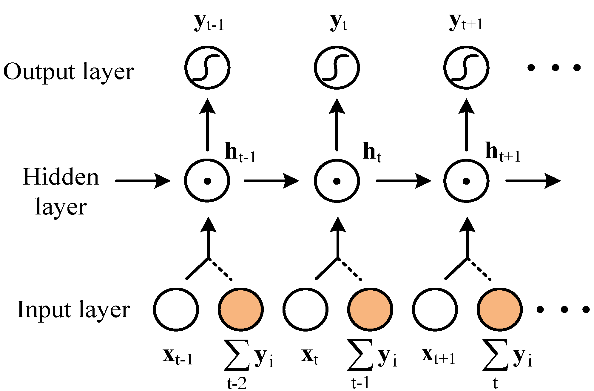
3.3. Classification Algorithm Based on IRRNN

3.3.1. IRRNN Overall Structure and Algorithm

Aiming at the sample dataset characteristics and classification requirements of the targets, this paper proposes an IRRNN model. On the one hand, to ensure that the periodic features of the sample sequence are preserved and not destroyed by truncation, we use the IndRNN structure, which has the ability to process longer sequences than the traditional RNNs structure. On the other hand, in order to improve the classification performance of the RNNs model, we use the RRNN model to map historical output information to the input layer through a random weight matrix.

The spatial point targets generally have micro-motion forms such as precession or tumbling in the exo-atmosphere, so that the infrared radiation intensity sequences have periodic characteristics, and different shapes and micro-motion features will be fully embodied in the sequences, which makes the traditional feature extraction methods hard to extract. Therefore, the RNNs model is suitable for the classification of target infrared radiation intensity sequences. The length of each input sequence determines whether the feature information can be completely input to the neural network. IndRNN makes the training simpler and more efficient because of its independent structure. At the same time, it solves the problem of gradient explosion and vanishing and can input longer sequences. Therefore, we use the IndRNN structure to make the periodic characteristic information of the sequence not lost and can be used for subsequent classification.

The infrared radiation intensity sequence of the spatial point target has high correlation in time, and the information before time step t has important reference value for the classification of current time. Therefore, we combine the historical output information before time step t by random weighting with the input data at time t and input it to the hidden layer for further processing.

The structure of the IRRNN is as shown in the following Figure 5. First, the historical output information is weighted by the random weight matrix W and combined with the input data of the current time together, and then becomes the new input data and enters the hidden layer. Then the neurons of the hidden layer are independent of each other, and the training is more efficient and stable and can effectively converge when the input sequence is long.

To reflect the structure of the IndRNN, the connection of the hidden layer is represented by the symbol of the Hadamard product $\odot$, and ReLU is used as the activation function.

Since the network structure of IRRNN improves the structure of the input layer and the connection mode of the hidden layer only on the basis of the traditional RNNs, the other network structures remain unchanged, so according to the Equations (8) and (14), the IRRNN network can be obtained. The calculation model is

$$\begin{array}{l}{{\mathbf{x}}^{\prime }}_t=\sigma \left({\mathbf{x}}_t+\beta {\displaystyle {\sum }_{i=1}^{t-1}{W}_i{\mathbf{y}}_i}\right);\\ {\mathbf{a}}_t={\mathbf{W}}^{\mathrm{HI}}·{{\mathbf{x}}^{\prime }}_t+\mathbf{w}\odot {\mathbf{h}}_{t-1}+{\mathbf{B}}^{\mathrm{H}};\\ {\mathbf{h}}_t=f_h({\mathbf{a}}_t);\\ {\mathbf{b}}_t={\mathbf{W}}^{\mathrm{OH}}·{\mathbf{h}}_t+{\mathbf{B}}^{\mathrm{O}};\\ {\mathbf{y}}_t=f_o({\mathbf{b}}_t),\end{array}$$

(17)

where $\odot$ indicates the Hadamard product, and other parameters are the same as Equation (14). In the formula, $f_h(·)$ and $f_o(·)$ are the activation function of the hidden layer and the output layer respectively. Because of the structure of IndRNN, $f_h(·)$ can be a unsaturated nonlinear function, so we choose ReLU as the activation function. And $f_o(·)$ still chooses Softmax as the activation function.

Through the above analysis of the IRRNN network structure, we use cross entropy as the loss function for the classification problem of the infrared radiation intensity time series of the spatial point target and use the gradient descent with momentum optimization method to update the network parameters during the training process. The specific training process of the IRRNN algorithm is shown in Algorithm 1. It is shown as follows:

Algorithm 1 Training process of time series classification algorithm based on IRRNN.

1. Determine network parameters: Number of neurons in the input layer of the IRRNN model network I, number of neurons in the hidden layer and backward transmission hidden layer H; Determine the error threshold for stopping training ε > 0; The total number of target time series in the sample set N. 2. Sample data preprocessing and parameter settings:    The training set, validation set, and testing set are divided according to 2:1:1, and generate random weighted matrix W1, W2,…, WT-1. 3. Initialize network weights and offset parameters:   Determine the initial value of WHI, w, WHO, BH, BO, etc. 4. Training process:    Assume that currently all N sequences in the training sample set for the kth pass, take sequence X(n) = [x1, x2, …, xT] as example     (1) For training sample xt at time step t, calculate the value of the network output value and loss function lt, etc.         $\begin{array}{l}{\mathbf{x}}_{\mathrm{t}}^{\prime }=\mathsf{\sigma }\left({\mathbf{x}}_{\mathrm{t}}+\mathsf{\beta }{\displaystyle {\sum }_1^{\mathrm{t}-1}{\mathbf{W}}_{\mathrm{i}}{\mathbf{y}}_{\mathrm{i}}}\right),\\ {\mathbf{a}}_{\mathrm{t}}={\mathbf{W}}^{\mathrm{HI}}·{\mathbf{x}}_{\mathrm{t}}^{\prime }+\mathbf{w}\odot {\mathbf{h}}_{\mathrm{t}-1}+{\mathbf{B}}^{\mathrm{H}},{\mathbf{h}}_{\mathrm{t}}={\mathrm{f}}_{\mathrm{h}}\left({\mathbf{a}}_{\mathrm{t}}\right),\\ {\mathbf{b}}_{\mathrm{t}}={\mathbf{W}}^{\mathrm{OH}}·{\mathbf{h}}_{\mathrm{t}}+{\mathbf{B}}^{\mathrm{O}},{\mathbf{y}}_{\mathrm{t}}={\mathrm{f}}_{\mathrm{o}}\left({\mathbf{b}}_{\mathrm{t}}\right),\\ {\ell }_{\mathrm{t}}=-{\mathbf{d}}_{\mathrm{t}}·\ln {\mathbf{y}}_{\mathrm{t}}.\end{array}$\     (2) Calculate the loss function for all time steps from 1 to T         ${\mathrm{E}}_{\mathrm{train}}={\displaystyle {\sum }_{\mathrm{t}=1}^{\mathrm{T}}{\ell }_{\mathrm{t}}}$     (3) Calculate the gradient of loss function Etrain to parameters $\nabla {\mathbf{W}}_{\mathrm{ji}}^{\mathrm{HI}}$, $\nabla {\mathbf{w}}_{\mathrm{ji}}^{}$, $\nabla {\mathbf{W}}_{\mathrm{ji}}^{\mathrm{OH}}$, etc.     (4) Update the network parameters by gradient descent with momentum optimization method, and obtain ${\mathbf{W}}_{\mathrm{j}\mathrm{i}}^{\mathrm{H}\mathrm{I}}\left(\mathrm{k}+1\right)$, ${\mathbf{W}}_{\mathrm{j}\mathrm{i}}^{}\left(\mathrm{k}+1\right)$, ${\mathbf{W}}_{\mathrm{j}\mathrm{i}}^{\mathrm{O}\mathrm{H}}\left(\mathrm{k}+1\right)$, etc.         $\begin{array}{l}{\mathbf{W}}_{\mathrm{j}\mathrm{i}}^{\mathrm{H}\mathrm{I}}\left(\mathrm{k}+1\right)={\mathbf{W}}_{\mathrm{j}\mathrm{i}}^{\mathrm{H}\mathrm{I}}\left(\mathrm{k}\right)+\mathrm{m}\left({\mathbf{W}}_{\mathrm{j}\mathrm{i}}^{\mathrm{H}\mathrm{I}}\left(\mathrm{k}\right)-{\mathbf{W}}_{\mathrm{j}\mathrm{i}}^{\mathrm{H}\mathrm{I}}\left(\mathrm{k}-1\right)\right)-\lambda \nabla {\mathbf{W}}_{\mathrm{j}\mathrm{i}}^{\mathrm{H}\mathrm{I}}\\ {\mathbf{W}}_{\mathrm{j}\mathrm{i}}^{}\left(\mathrm{k}+1\right)={\mathbf{W}}_{\mathrm{j}\mathrm{i}}^{}\left(\mathrm{k}\right)+\mathrm{m}\left({\mathbf{W}}_{\mathrm{j}\mathrm{i}}^{}\left(\mathrm{k}\right)-{\mathbf{W}}_{\mathrm{j}\mathrm{i}}^{}\left(\mathrm{k}-1\right)\right)-\lambda \nabla {\mathbf{W}}_{\mathrm{j}\mathrm{i}}^{}\\ {\mathbf{W}}_{\mathrm{j}\mathrm{i}}^{\mathrm{O}\mathrm{H}}\left(\mathrm{k}+1\right)={\mathbf{W}}_{\mathrm{j}\mathrm{i}}^{\mathrm{O}\mathrm{H}}\left(\mathrm{k}\right)+\mathrm{m}\left({\mathbf{W}}_{\mathrm{j}\mathrm{i}}^{\mathrm{O}\mathrm{H}}\left(\mathrm{k}\right)-{\mathbf{W}}_{\mathrm{j}\mathrm{i}}^{\mathrm{O}\mathrm{H}}\left(\mathrm{k}-1\right)\right)-\lambda \nabla {\mathbf{W}}_{\mathrm{j}\mathrm{i}}^{\mathrm{O}\mathrm{H}}\end{array}$     where m is momentum parameters, m [0, 1]; and λ is the learning rate, α $\in$ [0, 1].     (5) Enter the next sequence X(n’) in the training sample set and repeat the training process in steps (1) to (4) until all N sample sequences are processed through the network and proceed to the next step. 5. Stop the training, when the training error reaches the threshold. 6. Save the trained network parameters.

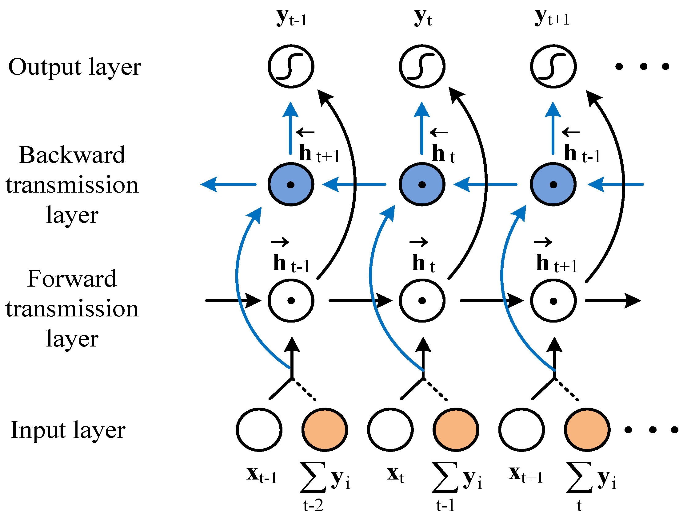
3.3.2. Bi-Direction Extension Structure of IRRNN

When the infrared radiation intensity time series of the spatial point target is processed according to the IRRNN structure of the previous section, only the data information before time step step t is used for the classification of decision processing at the current time, and the data information after time step t cannot be utilized. In fact, for the time series classification task of the spatial point target of this paper, due to the periodicity and continuity of the target motion, the sample data information before and after the current time step t is very important for the classification decision of the current time. Therefore, this paper proposes a Bi-direction IRRNN model, which makes the sample information change from the original forward-only transmission to a bidirectional network structure that can be forward and reverse. The sample information before and after time step t can be applied in the decision of the current state.

The network structure of the bidirectional IRRNN (B-IRRNN) is shown in Figure 6. As shown, there are two hidden layers that are independent of each other, and the input data is processed simultaneously in forward and backward manners. Then the output obtained is the weighted sum of results in two directions. It can be seen as a combination of two unidirectional RNNs networks, in particular, the hidden layer transmission of the two networks is reversed, and the output is determined by the results of the two networks together.

As shown in Figure 6, in the forward transmission layer, the hidden layer state $\overrightarrow{\mathbf{h}}$ is recursively calculated from t = 1 to T, and the corresponding output is $\overrightarrow{\mathbf{y}}$. In the backward transmission layer, the hidden layer state $\overleftarrow{\mathbf{h}}$ is inversely recursively calculated from t = T to 1, and the corresponding output is $\overleftarrow{\mathbf{y}}$. The final output is the weighted sum of the two output values. Therefore, the calculation formula of the B-IRRNN model is:

$$\begin{array}{c}{\overrightarrow{{\mathbf{x}}^{\prime }}}_t=\sigma \left({\mathbf{x}}_t+\beta {\displaystyle {\sum }_{i=1}^{t-1}{\mathbf{W}}_i{\overrightarrow{\mathbf{y}}}_i}\right),{\overleftarrow{{\mathbf{x}}^{\prime }}}_t=\sigma \left({\mathbf{x}}_t+\beta {\displaystyle {\sum }_{i=1}^{t-1}{\mathbf{W}}_i{\overleftarrow{\mathbf{y}}}_i}\right)\\ {\overrightarrow{\mathbf{h}}}_t=f_h\left({\overrightarrow{\mathbf{W}}}^{\mathrm{HI}}·{\overrightarrow{{\mathbf{x}}^{\prime }}}_t+\overrightarrow{\mathbf{w}}\odot {\overrightarrow{\mathbf{h}}}_{t-1}+{\overrightarrow{\mathbf{B}}}^{\mathrm{H}}\right),{\overleftarrow{\mathbf{h}}}_t=f_h\left({\overleftarrow{\mathbf{W}}}^{\mathrm{HI}}·{\overleftarrow{{\mathbf{x}}^{\prime }}}_t+\overleftarrow{\mathbf{w}}\odot {\overleftarrow{\mathbf{h}}}_{t-1}+{\overleftarrow{\mathbf{B}}}^{\mathrm{H}}\right)\\ {\overrightarrow{\mathbf{y}}}_t=f_o\left({\overrightarrow{\mathbf{W}}}^{\mathrm{OH}}·{\overrightarrow{\mathbf{h}}}_t+{\overrightarrow{\mathbf{B}}}^{\mathrm{O}}\right),{\overleftarrow{\mathbf{y}}}_t=f_o\left({\overleftarrow{\mathbf{W}}}^{\mathrm{OH}}·{\overleftarrow{\mathbf{h}}}_t+{\overleftarrow{\mathbf{B}}}^{\mathrm{O}}\right)\\ {\mathbf{y}}_t={\alpha }_1{\overrightarrow{\mathbf{y}}}_t+{\alpha }_2{\overleftarrow{\mathbf{y}}}_t,\end{array}$$

(18)

where α₁ and α₂ are the weighting coefficients of the output, and α₁ + α₂ = 1 is required. Considering that the information before and after the current time is equally important in the time series of the infrared radiation intensity of the target, the equal weight addition is used here, so α₁ = α₂ = 0.5. In the training process of B-IRRNN, the training parameters of the forward parameters ${\overrightarrow{\mathbf{W}}}^{\mathrm{H}\mathrm{I}},\overrightarrow{\mathbf{w}},{\overrightarrow{\mathbf{B}}}^{\mathrm{H}},{\overrightarrow{\mathbf{W}}}^{\mathrm{O}\mathrm{H}},{\overrightarrow{\mathbf{B}}}^{\mathrm{O}}$ and the backward parameters ${\overleftarrow{\mathbf{W}}}^{\mathrm{HI}},\overleftarrow{\mathbf{w}},{\overleftarrow{\mathbf{B}}}^{\mathrm{H}},{\overleftarrow{\mathbf{W}}}^{\mathrm{OH}},{\overleftarrow{\mathbf{B}}}^{\mathrm{O}}$ are respectively optimized, and the memory required is about twice the unidirectional IRRNN network.

4. Experiments and Discussion

The purpose of this section is to discuss the performance of the proposed IRRNN algorithm by conducting multiple sets of experiments. Firstly, the classification performance of the IRRNN algorithm for the UCR data set is tested. Then, the classification performance of the IRRNN algorithm model and its extended form B-IRRNN for the infrared radiation intensity time series of the spatial target are discussed.

4.1. URC Data Set Classification Experiment

Since the UCR public data set is widely used in time series processing problems, including time series data sets taken from different fields, some of the data sets are selected to test the performance of the proposed time series classification model based on IRRNN.

The experiment selected seven sequence data sets in the UCR for classification experiments. Four algorithms were used for comparison experiments, including the most basic feedforward neural networks (FNNs), traditional RNNs model, LSTM, and IRRNN proposed in this paper. The experiment uses the cross-validation method to determine the optimal network parameter values to prevent over-fitting phenomena that may occur during training. In addition, we performed 50 Monte Carlo simulations for each sample set, taking the average of all results as the final result. The accuracy of the classification for each data set by the four algorithms is shown in

Table 2. Classification accuracy of four algorithms in UCR data set.

Name	Sequence Length	Accuracy
		FNNs	RNNs	LSTM	IRRNN
ECG200	96	0.8189	0.8433	0.8650	0.8974
ArrowHead	251	0.7495	0.8012	0.8166	0.8285
SyntheticControl	60	0.7230	0.7432	0.7843	0.7812
OSULeaf	427	0.5823	0.6059	0.6337	0.6828
FaceAll	131	0.5541	0.5722	0.5870	0.6931
SwedishLeaf	128	0.7419	0.7692	0.7705	0.8131
FiftyWords	270	0.3932	0.4239	0.5152	0.6549

, and the algorithm with the highest classification accuracy for each data set is in bold.

As show in Table 2, it can be seen that the IRRNN model obtains the highest classification accuracy on the six data sets and is slightly lower than the LSTM model only on the “SytheticControl” data set. In general, the model classification performance based on RNNs is better than the basic feedforward neural network model, indicating that the recurrent structure of the neural network in time is very beneficial to the classification task of sequences. In the UCR data set classification task, the classification performance of LSTM is better than the RNNs model. However, the proposed IRRNN is more advantageous than the LSTM in the classification task. The independent structure solves the problem of gradient vanishing and explosion and can quickly converge to the optimal solution. The addition of random weighted history information makes the data tend to be easy to classify, and the network can be generalized. The validity and robustness of the IRRNN algorithm is teted by experiments.

4.2. Classification Experiment of Radiation Intensity Sequences

The experiment in this section mainly tests the proposed IRRNN classification model to classify the infrared radiation intensity sequences of spatial point targets and distinguishes them according to the different shapes of the target. According to the modeling analysis in Section 2, the specific parameters of the four types of targets are shown in Algorithm 1. In addition, in order to increase the difficulty of classification, we normalize all generated simulation sequences so that they are distributed between [0, 1]. This can enhance the diversity of the training sample set and also improve the robustness of the classification network to the target size parameters in retraining.

4.2.1. Classification Experiment

The infrared radiation intensity time series sample set of the spatial point target used in the experiment is obtained by modeling the real ballistic scene in Section 2, and the data length can be adjusted and changed. The classification performance of IRRNN algorithm can be tested at different moments in the case of data dynamic input. Considering that the observation of the target in the space infrared sensor may be obscured, and the data may be missing, we set the target sample sequence to be randomly acquired from 120 s to 300 s, and the sequence of the interception time is 30 s. The classification performance of algorithms are observed at times of 8 s, 16 s, 24 s from the start point of each sequence. The experiment was divided into three groups, and the performance of the classification algorithm with the beginning time tbeg of 150, 200, and 250 s was tested. Set the acquired sample data to a signal-to-noise ratio (SNR) level of 20 dB. The simulated infrared radiation intensity sequence sample data of the targets is 2000 sets, and the four types of targets each have 500 sets. Samples are randomly assigned to the training set, validation set and testing set according to the ratio of 2:1:1. So the number of samples for the training set is 1000, and the number of samples for the validation set and testing set is 500.

In this experiment, a separate IndRNN structure(2 layers) and RRNN structure were added to compare with the IRRNN structure and its bi-directional extended structure B-IRRNN. The purpose is to compare the effects of these two structures on classification performance. Traditional RNNs were used as a reference.

According to the classification algorithm performance in three groups of experiments as shown in

Table 3. Classification accuracy of four algorithms when t_beg = 150 s.

Observing Time (s)	Accuracy
	RNNs	IndRNN	RRNN	IRRNN	B-IRRNN
8	0.6375	0.8081	0.7729	0.8856	0.9124
16	0.7449	0.8424	0.8302	0.8987	0.9176
24	0.7892	0.8840	0.8743	0.9101	0.9315

,

Table 4. Classification accuracy of four algorithms when t_beg = 200 s.

Observing Time (s)	Accuracy
	RNNs	IndRNN	RRNN	IRRNN	B-IRRNN
8	0.6503	0.7985	0.7946	0.8822	0.9048
16	0.7455	0.8393	0.8420	0.8995	0.9109
24	0.7917	0.8867	0.8851	0.9098	0.9272

and

Table 5. Classification accuracy of four algorithms when t_beg = 250 s.

Observing Time (s)	Accuracy
	RNNs	IndRNN	RRNN	IRRNN	B-IRRNN
8	0.6416	0.7953	0.7864	0.8751	0.8939
16	0.7568	0.8413	0.8395	0.8903	0.9120
24	0.8059	0.8725	0.8874	0.9026	0.9234

, the following conclusions can be obtained:

(1) The classification accuracy of traditional RNNs algorithm improves with the increase of the sequence length. Because the RNN’s network can store the state information of the previous states and accumulate the historical history as the sequence length increases and the accuracy of classification of time series is also improved. However, although traditional RNNs have the ability of time-delay memory, the problem of degradation in parameter learning still exists. Only the sequence information in local time can be learned, and the long-term dependence of the sequence cannot be learned.

(2) IndRNN and RRNN have more advanced structures than traditional RNNs, and the classification performance is greatly improved compared with RNNs. The independent structure of IndRNN solves the problem of gradient vanishing and explosion, and can learn the long-term dependencies of sequences. For the RRNN structure, the historical output information uses the form of random weighting to make the new input data tend to the direction that is easy to classify.

(3) The classification performance of the IRRNN algorithm proposed in this paper is more prominent than the independent IndRNN algorithm and RRNN algorithm. Combining the advantages of both of them, the performance of the classification algorithm is significantly enhanced.

(4) The B-IRRNN model obtained the best classification performance at all observation times, and its classification accuracy was higher than that of the unidirectional IRRNN model. Because the B-IRRNN classification model has two hidden layers of forward propagation and backward propagation, it can simultaneously use past and future sequence information to help the classification decision at current time. It has more advantages than the unidirectional IRRNN model in time series classification.

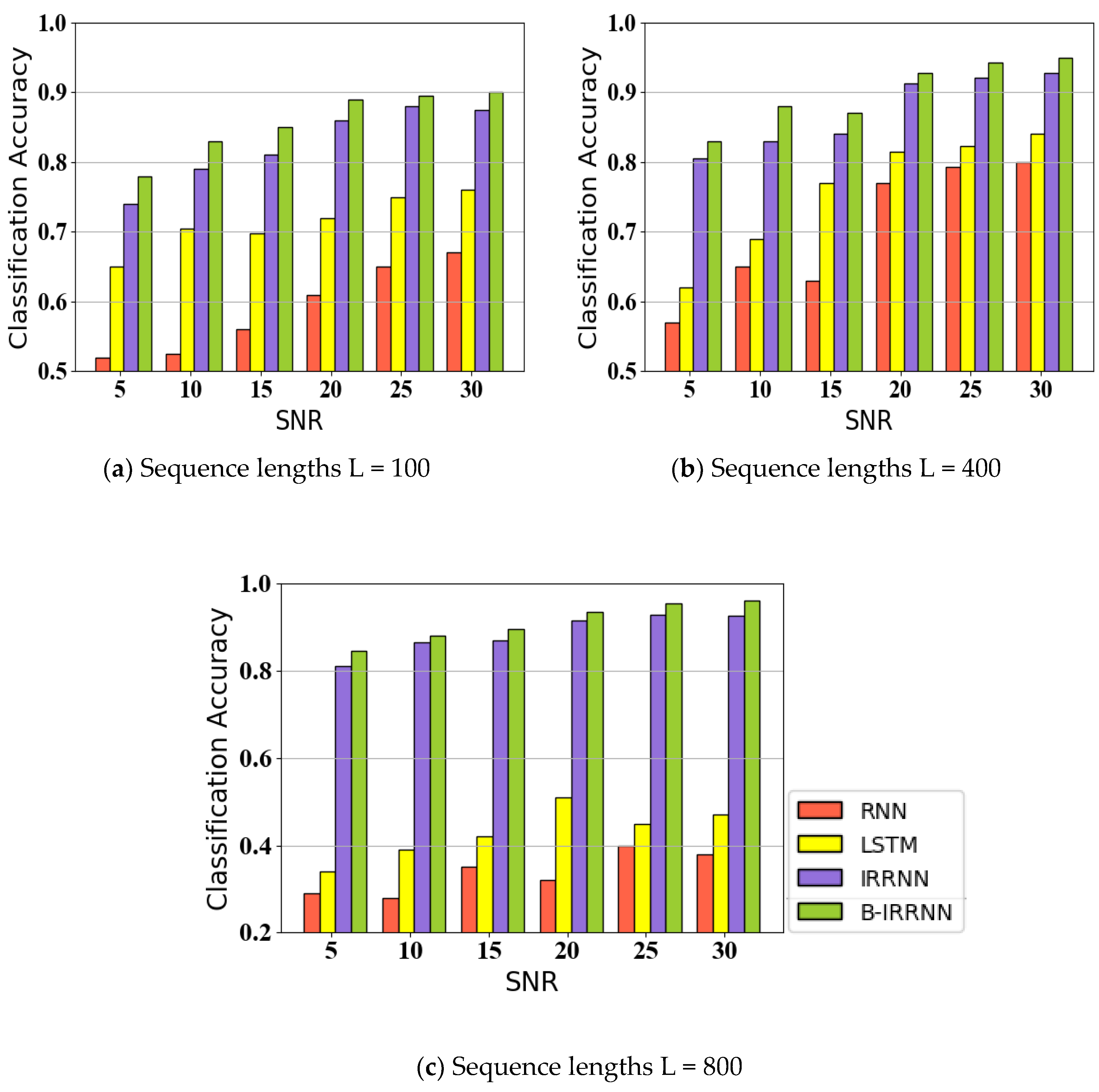
4.2.2. Effect of Noise and Sequence Length

The experiment mainly tests the classification performance of four algorithms including RNNs, LSTM, IRRNN, and B-IRRNN under the situation of different noise levels and different sequence lengths. In the training process, all the algorithms are trained with the same signal-to-noise ratio that is SNR = 20 dB and the same sequence length L = 400. Classification performance of infrared radiation intensity time series of spatial point targets by different algorithms are tested under different signal-to-noise ratio levels (5 dB, 10 dB, 15 dB, 20 dB, 25 dB, and 30 dB) and different input sequence lengths (200, 400, 600, 800, and 1000). Ten independent Monte Carlo simulation experiments were carried out, and the mean of the classification accuracy of each algorithm was taken as the final result. As shown in Figure 7, we can get the following conclusions:

(1) With the increase of SNR, the classification accuracy of each algorithm is obviously improved, indicating that noise is an important factor affecting the classification task of spatial point target based on radiation intensity sequence. Therefore, the selected classification algorithm must be robust to noise. Compared with traditional RNNs and LSTM, the proposed IRRNN algorithm and B-IRRNN algorithm have obvious advantages, and even in the case of high noise level, they have more stable classification ability and verify the robustness to noise.

(2) Comparing Figure 7a,b, it can be seen that the classification accuracy of four algorithms increases steadily with the increase of the sequence length, because the longer the sequence, the more periodic information of the target motion included and the more favorable to the classification of the sequence. It can be clearly seen from Figure 7c that when the sequence reaches a certain length, traditional RNNs and the LSTM cannot achieve effective classification of the sequence. This is because the problems of gradient vanishing and gradient explosion still exist, and their structure and activation function decided that a long sequence could not be processed. At this time, the advantage of the IRRNN algorithm and B-IRRNN algorithm are reflected. Their ability to process long sequences is strong, and the classification accuracy does not fluctuate greatly with the length of the sequence, remains at a relatively stable high level, and improves with the sequence length increases.

In summary, the IRRNN algorithm can process long sequences due to the independent structure of its hidden layer, which is beneficial to capturing the long-term periodic features of spatial point targets. The historical information is introduced into the input through random weighting simultaneously, which effectively improves the comprehensive classification performance of the algorithm and enhances the generalization capabilities of the network. In addition, the independent structure of the IRRNN algorithm simplifies the network parameters and calculations, and the random weighting of historical information does not increase the learning complexity of the network. Therefore, the IRRNN algorithm can accomplish the classification easily and efficiently. For the infrared radiation intensity time series classification task of the spatial point target studied in this paper, IRRNN can process long time sequences, achieve stable classification accuracy, be robust to noise, and output classification results in real time, which is in accordance with classification task requirements.

5. Conclusions

This paper proposes a time series classification model based on IRRNN. The infrared signature model of spatial point targets has been constructed as the premise, and samples of infrared radiation intensity sequences are achieved. Our model improves the abilities of avoiding gradient vanishing and explosion, processing long-length sequences, and classifying effectively. In addition, the bidirectional extension structure of IRRNN was carried out to obtain a better classification performance. Experiments show that our algorithm achieves higher classification accuracy under various sequence lengths and noise levels compared with RNNs and LSTM. The proposed IRRNN model can effectively solve the problem of infrared radiation intensity time series classification of spatial point targets.

References

1. Gronlund, L. Countermeasures to the US National Missile Defense. In Proceedings of the Aps April Meeting, Washington, DC, USA, 28 April–1 May 2001. [Google Scholar]
2. Resch, C.L. Neural network for exo-atmospheric target discrimination. Proc. SPIE Int. Soc. Opt. Eng. 1998, 3371, 119–128. [Google Scholar]
3. Chen, V.C.; Li, F.; Ho, S.S.; Wechsler, H. Micro-Doppler effect in radar: Phenomenon, model, and simulation study. IEEE Trans. Aerosp. Electron. Syst. 2006, 42, 2–21. [Google Scholar] [CrossRef]
4. Liu, J.; Li, Y.; Chen, S.; Lu, H.; Zhao, B. Micro-motion dynamics analysis of ballistic targets based on infrared detection. J. Syst. Eng. Electron. 2017, 28, 472–480. [Google Scholar]
5. Huang, L.; Li, X.; Liu, J. IR radiative properties modeling and feature extraction method on ballistic target. In Proceedings of the Seventh International Conference on Digital Image Processing (ICDIP 2015), Los Angeles, CA, USA, 9–10 April 2015. [Google Scholar]
6. Qiu, C.; Zhang, Z.; Lu, H.; Zhang, K. Infrared modeling and imaging simulation of midcourse ballistic targets based on strap-down platform. Syst. Eng. Electron. 2014, 25, 776–785. [Google Scholar] [CrossRef]
7. Wang, H.Y.; Zhang, W.; Wang, F.G. Visible characteristics of space-based targets based on bidirectional reflection distribution function. Sci. China Technol. Sci. 2012, 55, 982–989. [Google Scholar] [CrossRef]
8. Li, F.; Xu, X. Modeling Time-Evolving Infrared Characteristics for Space Objects with Micromotions. IEEE Trans. Aerosp. Electron. Syst. 2012, 48, 3567–3577. [Google Scholar] [CrossRef]
9. Liu, L.; Du, X.; Ghogho, M.; Hu, W.; McLernon, D. Precession missile feature extraction using the sparse component analysis based on radar measurement. EURASIP J. Adv. Signal Process. 2012, 24. [Google Scholar] [CrossRef]
10. Wang, J.; Yang, C. Exo-atmospheric target discrimination using probabilistic neural network. Chin. Opt. Lett. 2011, 9, 070101. [Google Scholar] [CrossRef]
11. Bengio, Y. Learning deep architectures for AI. In Foundations Trends Machine Learning; Now Publishers Inc: Hanover, MA, USA, 2009; Volume 2, pp. 1–27. [Google Scholar]
12. Graves, A. Supervised Sequence Labeling with Recurrent Neural Networks; Springer: New York, NY, USA, 2012. [Google Scholar]
13. Ma, Y.; Chang, Q.; Lu, H.; Liu, J. Reconstruct Recurrent Neural Networks via Flexible Sub-Models for Time Series Classification. Appl. Sci. 2018, 8, 630. [Google Scholar] [CrossRef]
14. Pascanu, R.; Mikolov, T.; Bengio, Y. On the difficulty of training recurrent neural networks. In Proceedings of the International Conference on Machine Learning, Atlanta, GA, USA, 16–21 June 2013. [Google Scholar]
15. Hammer, B. On the approximation capability of recurrent neural networks. Neurocomputing 2000, 31, 107–123. [Google Scholar] [CrossRef]
16. Hochreiter, S.; Schmidhuber, J. Long short-term memory. Neural Comput. 1997, 9, 1735–1780. [Google Scholar] [CrossRef] [PubMed]
17. Graves, A.; Beringer, N.; Schmidhuber, J. Rapid Retraining on Speech Data with LSTM Recurrent Networks; Technical Report No. IDSIA–09–05; Instituto Dalle Molle di studi sull’ intelligenza artificiale: Manno, Switzerland, 2005. [Google Scholar]
18. Pierre, B.; Soren, B.; Paolo, F.; Gianluca, P.; Giovanni, S. Bidirectional Dynamics for Protein Secondary Structure Prediction. Seq. Learn. Paradig. Algorithms Appl. 2000, 21, 99–120. [Google Scholar]
19. Baldi, P.; Brunak, S.; Frasconi, P.; Pollastri, G.; Soda, G. How to construct deep recurrent neural networks. In Proceedings of the International Conference on Learning Representation, Banff, AB, Canada, 14–16 April 2014. [Google Scholar]
20. Li, S.; Li, W.; Cook, C.; Zhu, C.; Gao, Y. Independently Recurrent Neural Network (IndRNN): Building A Longer and Deeper RNN. Comput. Vis. and n.a. Recognit. 2018. [Google Scholar] [CrossRef]
21. Linares, R.; Jah, M.; Crassidis, J.L.; Christopher, K.N. Space object shape characterization and tracking using light curve and angles data. J. Guid. Control Dyn. 2014, 37, 13–26. [Google Scholar] [CrossRef]
22. Wu, Y.; Lu, H.; Zhao, F.; Zhang, Z. Estimating Shape and Micro-Motion Parameter of Rotationally Symmetric Space Objects from the Infrared Signature. Sensors 2016, 16, 1722. [Google Scholar] [CrossRef] [PubMed]
23. Liu, J.; Chen, S.; Lu, H.; Zhao, B. Ballistic targets micro-motion and geometrical shape parameters estimation from sparse decomposition representation of infrared signatures. Appl. Opt. 2017, 56, 1276–1285. [Google Scholar] [CrossRef] [PubMed]
24. Liu, J.; Chen, S.; Lu, H.; Zhao, B. Nutation characteristics analysis and infrared signature simulation of ballistic targets. In Proceedings of the Advanced Information Technology, Electronic and Automation Control Conference, Chongqing, China, 25–26 March 2017; pp. 1001–1005. [Google Scholar]
25. Wetterer, C.J.; Jah, M. Attitude estimation from light curves. J. Guid. Control Dyn. 2009, 32, 1648–1651. [Google Scholar] [CrossRef]
26. Kaasalainen, M.; Torppa, J. Optimization methods for asteroid light-curve inversion I: Shape determination. Icarus 2001, 153, 24–36. [Google Scholar] [CrossRef]
27. Kohonen, T. Self-Organizing Maps; Springer: Berlin, Heidelberg, 2001. [Google Scholar]
28. An, G. The effects of adding noise during back-propagation training on a generalization performance. Neural Comput. 1996, 8, 643–674. [Google Scholar] [CrossRef]
Figure 1. Geometry of IR sensor and a target with nutation, where the IR detection coordinates are parallel to the reference coordinates.
Applsci 09 04622 g001
Figure 2. Infrared radiation intensity sequence of four shapes of spatial targets.
Applsci 09 04622 g002
Figure 3. MSE of LSTM and IndRNN with different sequence lengths.
Applsci 09 04622 g003
Figure 4. The structure of RRNN unfolded by time.
Applsci 09 04622 g004
Figure 5. Structure of IRRNN model unfolded by time.
Applsci 09 04622 g005
Figure 6. Structure of B-IRRNN model unfolded by time.
Applsci 09 04622 g006
Figure 7. Classification performance of four algorithms under the situations of different SNR sequence lengths.
Applsci 09 04622 g007