1. Introduction
Water depth is one of the basic elements of seabed topographic mapping and marine environment survey. The key and basic data provided by water depth monitoring are used in coastal engineering construction, ship navigation, and island development and utilization. The traditional bathymetric method of using ship-borne echo sounding achieved remarkable success. However, survey vessels and surveyors cannot easily carry out the traditional methods in shallow water (0–2 m) due to the influence of tide and submerged reef, indicating a restriction of these methods. Compared with traditional onsite acoustic measurements, the remote sensing inversion of water depth has the advantages of synchronous measurement in large coverage areas, high efficiency, and low cost. Remote sensing is an effective complement to traditional bathymetric methods in places where underwater terrains are complicated and unstable, and in sea areas affected by issues with rights and conflicts of interest.
The remote sensing inversion models of water depth can be divided into three types: Theoretical models [
1,
2], semi-empirical and semi-theoretical models [
3,
4,
5], and empirical models [
6,
7]. Among them, theoretical models need several physical parameters, including water environment, seabed sediment, and atmospheric environment. On the one hand, remote sensing images usually take the form of historical data, and deriving the physical parameters of synchronous images is difficult. On the other hand, morbidity inversion is a serious issue owing to the excessive number of physical parameters. Empirical models use a large amount of water depth data collected onsite and establish functional relations in the gray levels of remote sensing image bands for data inversion, but physical environment parameters, such as atmosphere and water quality, are ignored. Although the empirical models are relatively uncomplicated, their universality is poor, and executing them in inaccessible sea areas is difficult. Semi-empirical and semi-theoretical models combine the advantages of the above two models. These models can simultaneously model the radiation transfer of sunlight in water and use a small amount of field depth data to complete the inversion of water depth. In view of this advantage, the semi-empirical and semi-theoretical models are presently the most mainstream method of water depth inversion. However, the restive nature of acquiring in situ data for islands and reefs far from the mainland, particularly those parts that are difficult or inappropriate to reach, is regarded a crucial bottleneck in the inversion of water depth.
Airborne light detection and ranging (LiDAR) bathymetry can effectively and efficiently measure shallow waters and oceans, but the advantages are more obvious in areas inaccessible to surveying vessels. LiDAR bathymetry is widely used in the field of modern ocean bathymetry because of its high accuracy, efficiency, and mobility. However, LiDAR bathymetry relies on an aircraft platform, which is expensive. Therefore, the combination of passive remote sensing with a small amount of LiDAR waveform data can not only reduce the cost of depth inversion but also complete the high-precision inversion of depth data in sea areas that are difficult or inappropriate to reach.
2. Related Work
The bathymetric system of LiDAR matured as a technology in recent years. However, the data processing software of the bathymetric system is limited to some extent, and bathymetric accuracy is affected by the processing of waveform data, which are affected by bottom reflection, suspended matter, and sea waves [
8]. The bathymetric algorithm of the LiDAR waveform accordingly became a research focus of many scholars. The bathymetric inversion methods mainly include the peak detection method [
9,
10], mathematical function fitting method [
11,
12,
13], and convolutional filtering method [
14,
15,
16]. Billard [
17] proposed a method to detect seabed reflection signal by removing the low-frequency part of the echo signal through high-pass filtering. Wagner [
9] employed the peak detection method to search the echo signal from the surface and the bottom of the sea, and the method was found to be feasible. Wong [
18] decomposed two kinds of independent reflection signals, namely, sea surface echo signals and sea bottom echo signals, from which water depth was then estimated. Chen [
19] improved the inversion accuracy of water depth by using the phase ambiguity resolution technique to correct wave and tide measurements. Yao [
20] established a LiDAR echo waveform model based on the bi-Gaussian pulse fitting method and applied it to separate surface and bottom reflection signals. A minimum depth of 0.4 m was retrieved from their study. Zhang [
21] utilized a Gaussian function entailing the double fitting of simulated waveform data to retrieve water depth. Their results showed that a mean absolute error (MAE) of 15.6 cm and a mean relative error (MRE) of 4.58% could be achieved at the water depth of 1–15 m using the LiDAR depth-detection model. In practice, a portion of the LiDAR effective signal leaches and the low-frequency signal is removed when using a filtering method, but the error is larger and the efficiency rate is slower when a peak detection method is used directly. The resultant fitting effect is unsatisfactory for deep waters due to the large energy gap between the echo signals from the sea surface and the sea bottom. Moreover, the bathymetric inversion error for deep waters is greater than that in shallow waters.
The accuracy of depth inversion by passive remote sensing is lower than that by LiDAR. Meanwhile, bathymetric retrieval by active optical remote sensing has high precision and maneuverability. Consequently, bathymetric retrieval methods based on active and passive remote sensing were studied in recent years. Pacheco [
22] utilized the multi-band logarithmic linear model and Landsat 8 remote sensing image to invert shallow water depths (0–12 m) in areas around islands. The inversion algorithm of passive optical remote sensing was optimized using LiDAR bathymetric data. The average error of the inversion results was 0.2 m, and the median error was 0.1 m. Tian [
23] carried out bathymetric retrieval by active and passive remote sensing with the use of a passive optical image from Landsat-8 and airborne LiDAR depth data, and subsequently analyzed the results of different density LiDAR data for depth inversion by passive optical sensing. Their results showed that the change in LiDAR density only minimally affected the water depth inversion results, and the average relative error changed by 0.3%. Many scholars also conducted substantial research and experiments on sediment classification and topographic mapping using active and passive remote sensing data [
24,
25,
26]. Depth inversion by active and passive remote sensing can not only improve the accuracy of passive optical depth inversion, but also reduce the use of active optical data, as well as reduce costs.
On the basis of the above discussions, this study takes Ganquan Island as an example and uses the bathymetric values extracted from Aquarius LiDAR waveform data. Multi-Gaussian function fitting is performed to derive the control points and validation points, and the bathymetric method of combining active and passive remote sensing is carried out in the sea area around islands far from the mainland.
3. Materials and Methods
3.1. Research Area and Data
3.1.1. Research Area
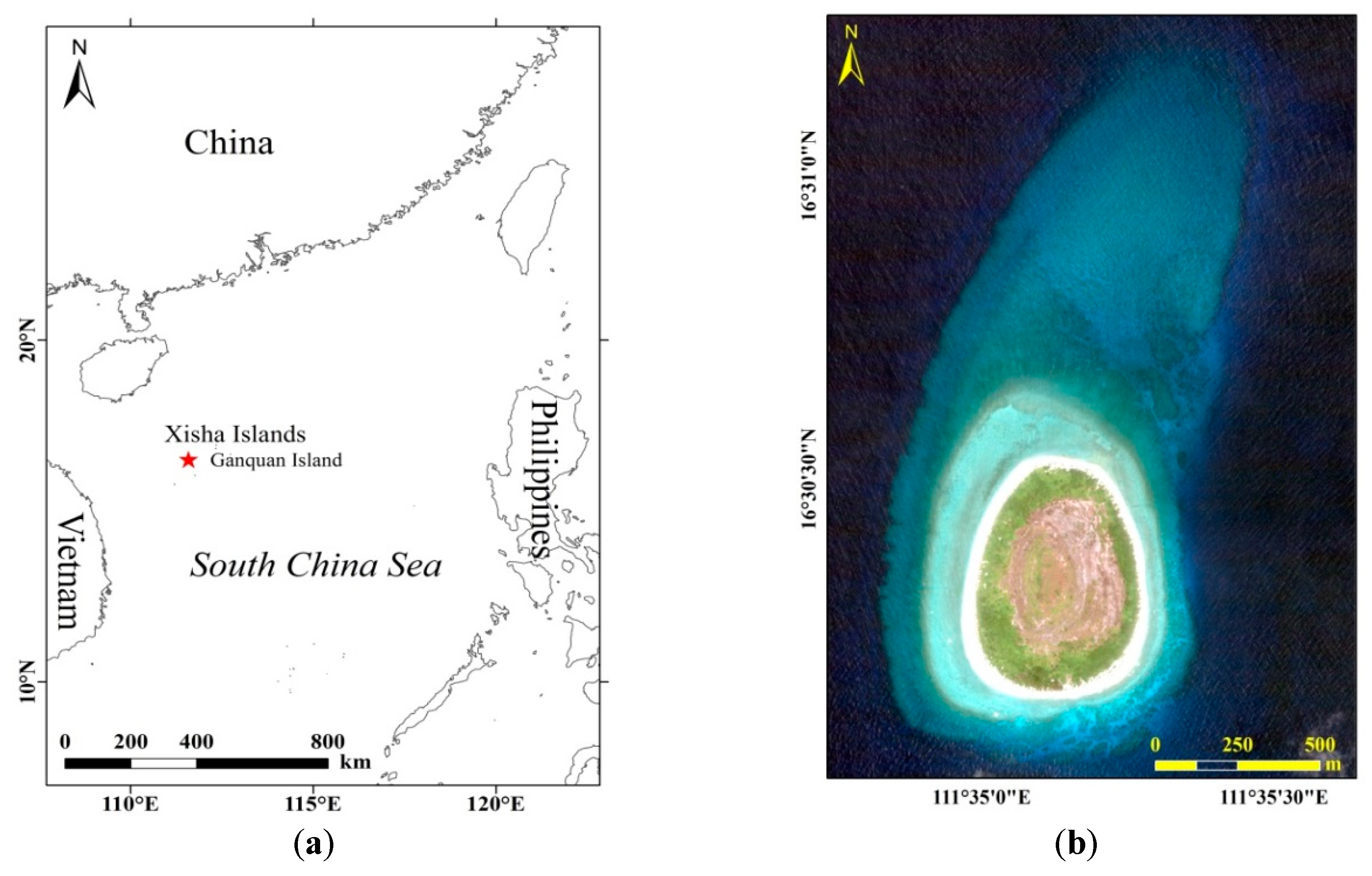
Ganquan Island (111°35′10″ east longitude and 16°30′28″ north latitude) belongs to the Xisha Islands in China. The island has a tropical monsoon climate, and it is approximately 500 m from east to west (width) and 700 m from north to south (length), with an area of approximately 0.3 km
2. The waters around Ganquan Island are clear and limpid and largely unaffected by human activities. The study area and multispectral image are shown in the
Figure 1a,b respectively.
3.1.2. Aquarius LiDAR Waveform Data
The Aquarius LiDAR bathymetry system (Optech Company, Canada) is an amphibious measuring system for shallow sea areas which can measure both land information and shallow water information within 15 m. The bathymetry system uses a blue-green laser (532 nm). The specific parameters are shown in
Table 1.
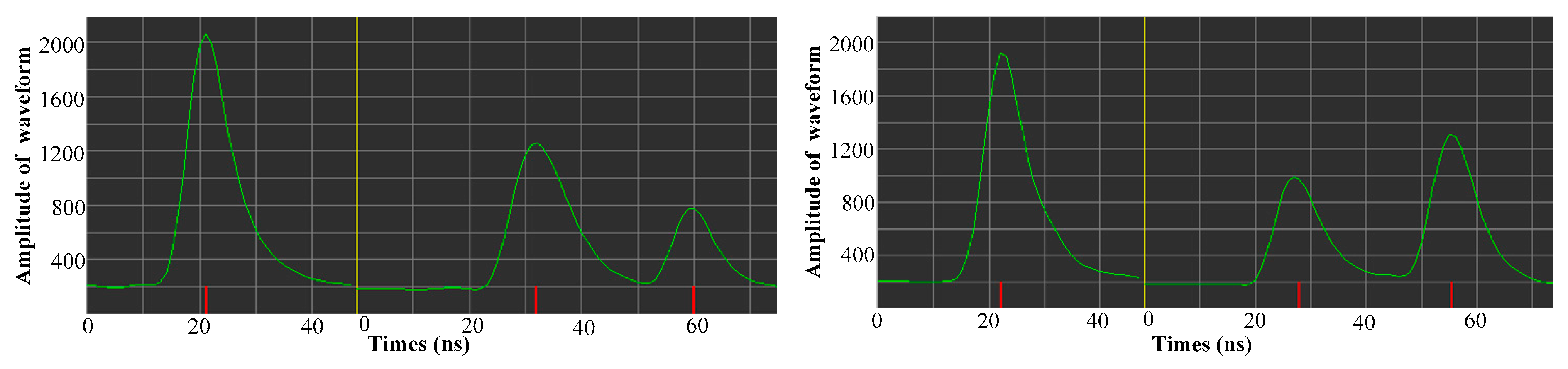
The waveform data obtained by an Aquarius-airborne LiDAR were acquired from the findings of an onsite survey conducted on 19 January 2013. Flight time was approximately 3 h, and total data volume was approximately 55 GB. The information stored in each waveform data included reflected pulse signals, received pulse signals, and GPS time. The left side of the yellow vertical line in
Figure 2 represents the transmitting pulse, while the right side represents the receiving pulse. Different targets or regions appear with varying return signal characteristics, mainly in terms of energy value, shape, and quantity of echo signals.
3.1.3. QuickBird Passive Optical Image
The QuickBird satellite provides a panchromatic band with 0.61-m spatial resolution and a multi-spectral image with 2.44-m spatial resolution, as shown in
Table 2. The passive optical image adopted in this study was the multispectral image (
Figure 1b). The image acquisition time was 2:31:52 a.m. (Coordinated Universal Time, UTC) on 20 April 2012.
3.1.4. Auxiliary Data
The auxiliary data used in this study mainly included tide tables for the period covering 2012 and 2013 published by National Marine Scientific Data Center. The time period of the LiDAR data measured onsite was approximately 3 h, and the tides changed considerably during those periods. Therefore, performing a tidal correction on each water depth value converted from the waveform data was necessary to ensure the accurate use of control points and validation points.
3.2. Data Processing and Method
For the LiDAR waveform data, we propose a multi-Gaussian function fitting method to extract water depth. The bathymetric values were converted into mean lower low water (MLLW) data to unify the standards of measurement. A series of preprocessing steps for the QuickBird image, such as radiation calibration and atmospheric correction, were needed. The improved logarithmic conversion ratio model (ILCRM) was used for the active and passive combination of water depth inversion in this study.
3.2.1. QuickBird Image Preprocessing
1. Radiation calibration
The ground object signals received by satellite sensors are recorded with a dimensionless Digital Number (DN) value, and the process of converting the DN value into a radiation brightness value with practical physical significance is called radiation calibration. The basic principle of radiometric calibration is to establish the quantitative relationship between the DN value and the radiation brightness value in the corresponding field of view.
The calibration formula for the remote sensing image of QuickBird is
where
L is the inputted pupil radiation brightness of the sensor,
DN is the pixel gray value,
absCalFactor is the absolute scaling factor, and
effectiveBandwidth is the effective width of the spectrum. The information on absolute calibration factor and effective spectral width can be found in the calibration file (*.IMD). The details are listed in
Table 3.
After radiometric calibration, the QuickBird remote sensing image is converted from one with the original dimensionless DN into one with a radiance value with units.
2. Atmospheric correction
Satellite sensors are affected by the scattering and absorption of atmospheric particles, aerosols, and molecules in the process of receiving solar photoelectric and electromagnetic radiation. The effects of scattering attenuate the signals received by the sensors. Meanwhile, some of the scattered light from the sky directly penetrates the satellite sensor without interacting with ground objects. This part of the signal does not contain any ground object information; we call this phenomenon atmospheric path radiation. Therefore, the atmospheric effects need to be eliminated to obtain highly realistic ground radiation or reflectance.
The atmospheric correction method used in this study was the 6S model method. The 6S model, which is the abbreviation of second simulation of the satellite signal in the solar spectrum, was developed by adding a new scattering algorithm based on the 5S model and, thus, can better reflect the real situation than the LOW resolution atmospheric TRANsmission (LOWTRAN) and MODerate resolution atmospheric TRANsmission (MODTRAN) models.
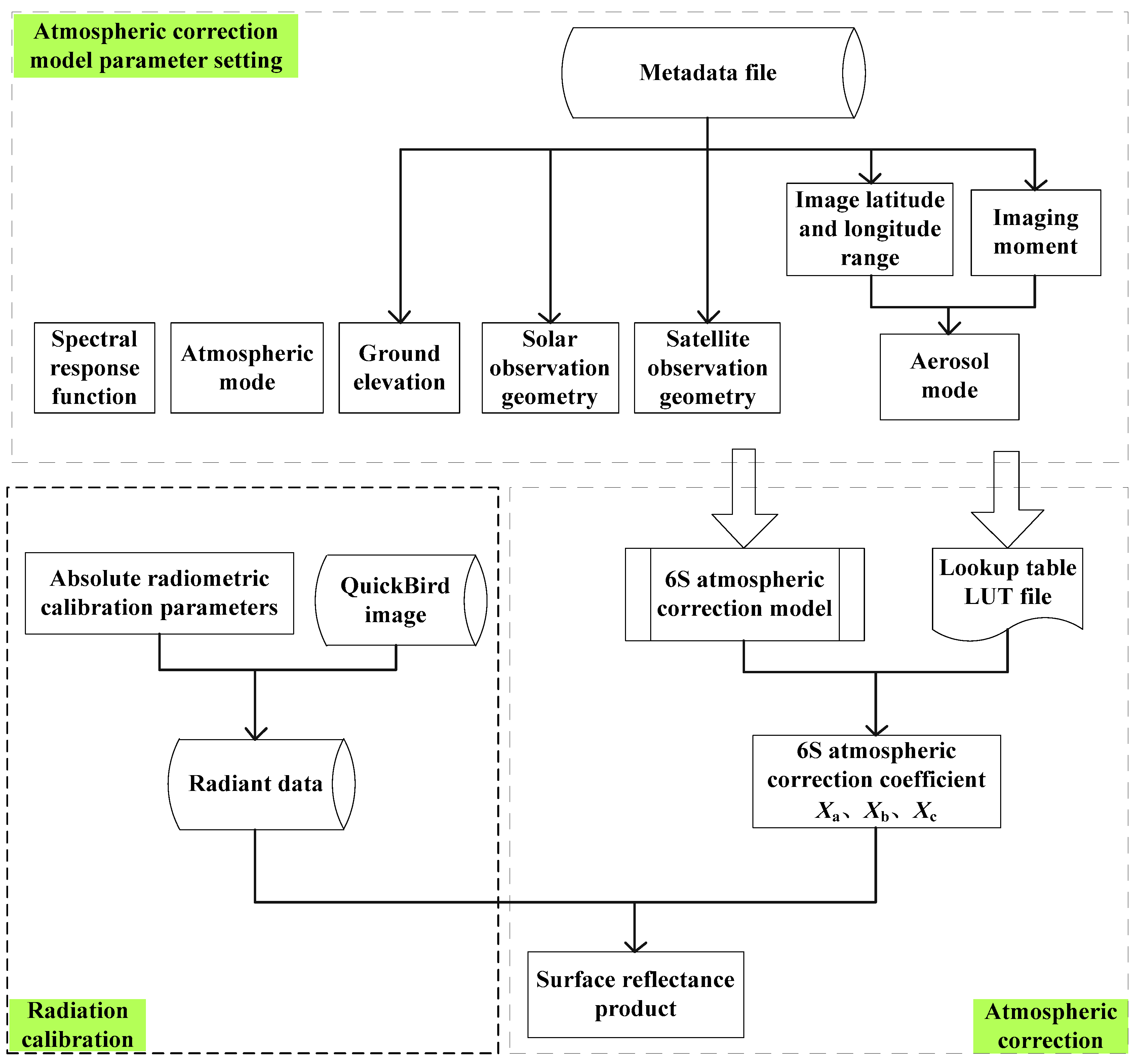
Figure 3 shows the technical route of the 6S atmospheric correction that consists of three parts: Parametric setting of the atmospheric correction model, radiation calibration, and atmospheric correction [
27].
The parameters of the 6S atmospheric correction model were set as follows: Ground elevation, solar observation geometry, satellite observation geometry, and other parameters obtained directly from the *.IMD file corresponding to the metadata of the remote sensing image; the spectral response function obtained from the data disclosed by the sensor; the atmospheric model parameters with default values obtained according to the remote sensing image data, mainly in the aerosol mode, atmospheric mode, and solar spectrum function; and a customization of the actual situation. We selected marine aerosol and tropical atmospheric mode in accordance with the needs of the study area.
After radiation calibration, the DN value of the remote sensing image is converted into an apparent radiation brightness value, followed by a conversion into an apparent reflectance value by Equations (2) and (3). Apparent reflectance is the ratio of radiation brightness at the entrant pupil of the satellite sensor to the descending sun brightness on top of the atmosphere, which also includes the role of the atmosphere.
where
is the apparent emissivity,
is the relative distance between the sun and the earth, and
is the average solar radiation value of the band with the unit
. The value of
can be calculated according to the spectral response function of the satellite sensor. The calculation formula is
where
and
are the spectral wavelengths of the sensor with the unit
, and
is the solar radiation value outside the atmosphere with the unit
. Equation (3) can be calculated from the solar spectrum response function provided by the World Radiation Center.
After the model parametric setting is completed, the 6S atmospheric correction model can be run to obtain the atmospheric correction parameters of
,
, and
. Subsequently, the apparent reflectance data of the image are converted into surface reflectance data. The conversion formulas are as follows:
where
is the surface reflectance, and
,
, and
are the conversion parameters calculated by the 6S atmospheric correction model. The desired surface reflectance data were, thus, obtained.
3.2.2. Water Depth Inversion Model
1. Principle of bathymetry based on passive optical remote sensing
Sunlight has a perspective in a water column. The signal received by the optical remote sensor contains reflection information of the sea bottom to the sunlight, and this information is the physical basis of the passive optical remote sensing inversion of shallow water depth. In other words, the information reflected from the seabed to the optical remote sensor is the direct reflection of underwater terrain, that is, the information source of optical remote sensing bathymetry. The attenuation coefficient of sunlight in water determines the penetrable depth of the light in water. The smaller the attenuation coefficient of light in water is, the better its transparency in water is. This phenomenon is the basic principle of water depth inversion.
In the process of radiation transmission, a series of complicated changes take place in the light after sunlight passes through the atmosphere and the water column, then to the bottom of the water, before finally entering the satellite sensor. As shown in
Figure 4, the satellite sensor receives the radiation signal
mainly in four parts.
where
is the atmospheric radiation,
is the reflection radiance of the water surface,
is the water column radiance, and
is the bottom radiance. The radiative transfer equation of electromagnetic waves in water is the physical basis of water depth inversion. Lyzenga [
28,
29] and Philpot [
30] developed the water depth radiation transfer equation according to Beer’s law.
where
is the radiative brightness value after atmospheric correction and radiative brightness correction of the water column in deep water,
is the radiation brightness value at infinite depth,
is the two-way diffuse attenuation coefficient in the water body,
is the water depth value, and
is the reflected energy value of the bottom.
2. Remote sensing bathymetric model
The radiation transfer equation and the basic principle of water depth inversion led to the rapid development of the bathymetric method, which mainly comprises the theoretical analytical model [
31], single-band water depth inversion model [
32,
33], multi-band log-linear model [
34,
35,
36], and logarithmic conversion ratio model [
37]. Tian [
4] improved the method on the basis of the classic Stumpf model to significantly improve water depth inversion ability. Considering the risk that the denominator of the Tian model may be equal to zero, we added the constant factor
a to the bathymetric model. The
a value may not increase model accuracy, but it can increase the stability of the model to a certain extent. The passive optical remote sensing bathymetric model used in this study was named ILCRM, expressed as follows:
where
Z is the water depth,
and
are the reflectance data of the blue and green bands, respectively,
and
are regression coefficients,
and
are the adjustment factors, and
a is the added constant factor (i.e., users can customize its value, such as setting it to 1.01). Because blue and green bands have strong transmission ability to water body, the signals received by sensors contain seabed information; thus, the two bands were used in this study. This method belongs to the classification of semi-empirical and semi-analytical models. A part of the water depth obtained from LiDAR waveform data was used as the control point to calculate the model parameters of
,
,
, and
. The other part of the water depth data was used as the validation point to evaluate the accuracy of the bathymetric model.
3.2.3. LiDAR Waveform Processing
1. Depth extraction from waveform data
Extracting the signals of the water surface and the bottom part from an echo waveform is the key to retrieving bathymetry based on the LiDAR waveform. The retrieving methods and parameters of the sounding system were not disclosed, but they seem to apply the commonly used peak detection method [
9,
18] and mathematical fitting method [
12,
38,
39]. A burr phenomenon always exists in the echo waveform signals arising from noise. A big error occurs when the peak detection method is directly used to extract the time in which the echo signals return to the water surface and the bottom. The method of filtering, denoising, and processing affects the response of the water component to the seabed waveform. Although the water component is not the focus of our extraction, it has great influence on the seabed waveform. By analyzing the radiation transmission of LiDAR in water bodies [
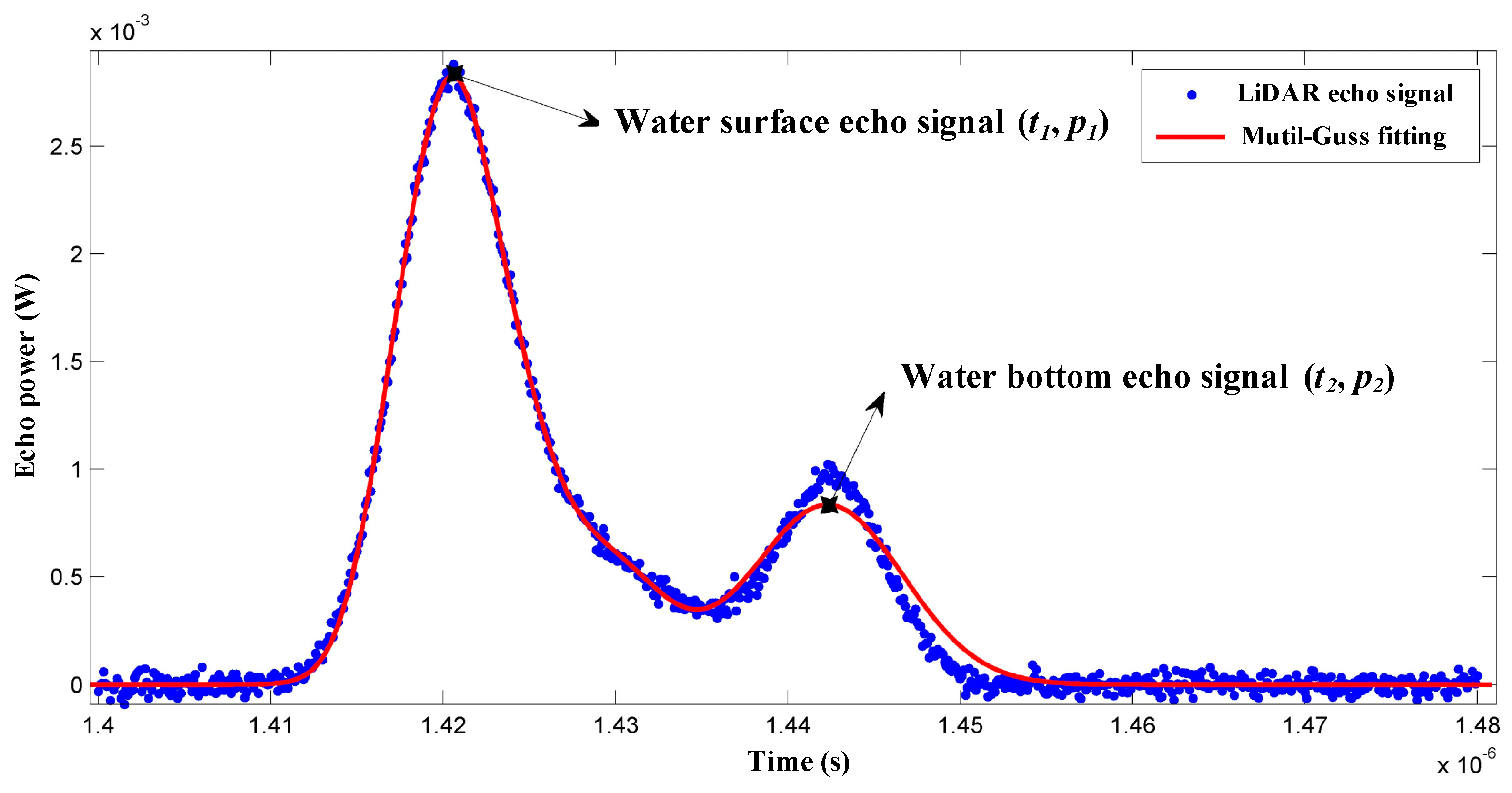
11], we find that the received echo signals approximate a Gaussian distribution [
21,
39]; thus, we use the multi-Gaussian function fitting to extract the target echo signal.
where
is the fitting curve expression based on the Gaussian function,
and
are the parameters of the function,
i is the number of Gaussian function,
d is the correction parameter, and
t is time.
We construct the objective function as
where
is the start time of the echo signal reception, and
is the end time of the echo signal reception.
The Levenberg–Marquardt algorithm is used to solve the optimization problem as follows:
Given a reasonable initial value, we can derive the coefficient
after optimal operation and then use the peak detection method to extract the peak position of the fitting curve for the echo signals of the water surface and the bottom part as
and
, respectively. The expression of the peak detection method is shown in Equation (12). The difference between the
x-coordinates of the two peak values is the time difference of the return of echo signal from the water surface and the bottom. The bathymetry can be calculated as shown in Equation (13).
where
is the sum of the Gaussian function used to iterate and fit the LiDAR echo signal,
is the difference between two consecutive points, i.e.,
;
is a sign function to depict whether the input value is negative, positive, or zero, in which the return value is −1, 1, or 0, respectively,
returns the indices of the elements to satisfy the expressions inside it,
is the speed of light in water, and
is the local incidence angle in water. The blue points in
Figure 5 represent the echo signals of LiDAR, while the red curve represents the fitting curve based on the Gaussian function.
2. Datum conversion
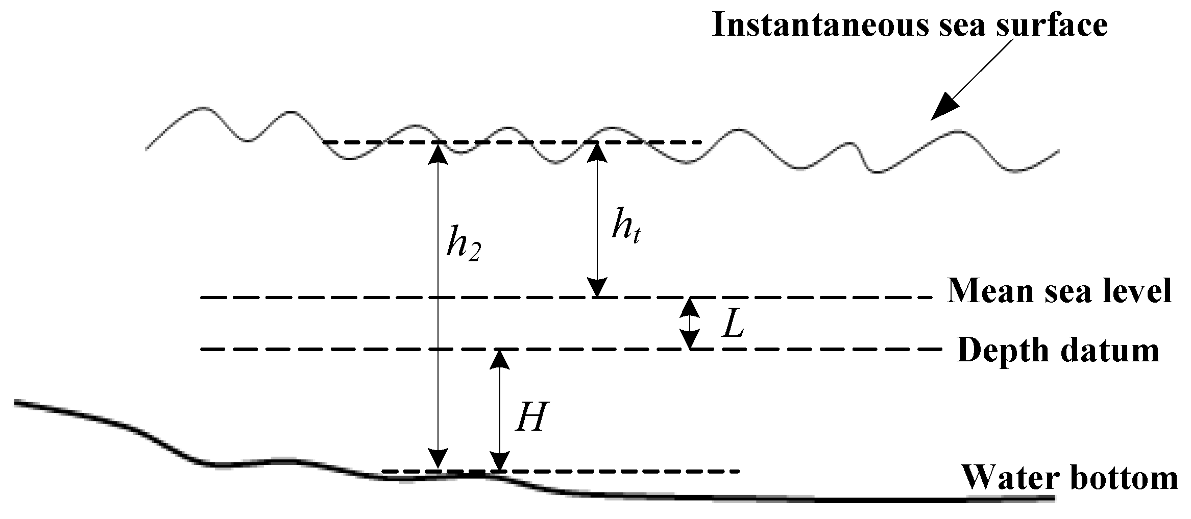
The bathymetry obtained by resolving the LiDAR waveform corresponds to instantaneous water depth. The bathymetric data need to be corrected by using tide data to derive the water depth value for the acquisition time of the optical remote sensing image. The relationship of instantaneous sea surface, mean sea level, depth, and water bottom is shown in
Figure 6. However, the LiDAR data were acquired from 11:00 a.m. to 2:00 p.m. on 19 January 2013, and the collection time of each point differed. Therefore, performing a tide correction for each control point and validation point is necessary to eliminate the errors caused by different tides.
The LiDAR bathymetry data were calculated using the same reference surface as the optical image for the satellite-derived bathymetry. MLLW data (referring to the depth data in the
Figure 6) are commonly used as the reference for bathymetric mapping. Therefore, MLLW data were selected as the starting surface. The conversion formula is as follows:
4. Results
Bathymetric inversion around Ganquan Island was carried out based on the LiDAR waveform data and the QuickBird image. We compared the depth detected by the multi-Gaussian function and the LiDAR processing software. Moreover, the inversion capability from combining active and passive remote sensing was evaluated from the aspects of overall accuracy and specific depth range accuracy.
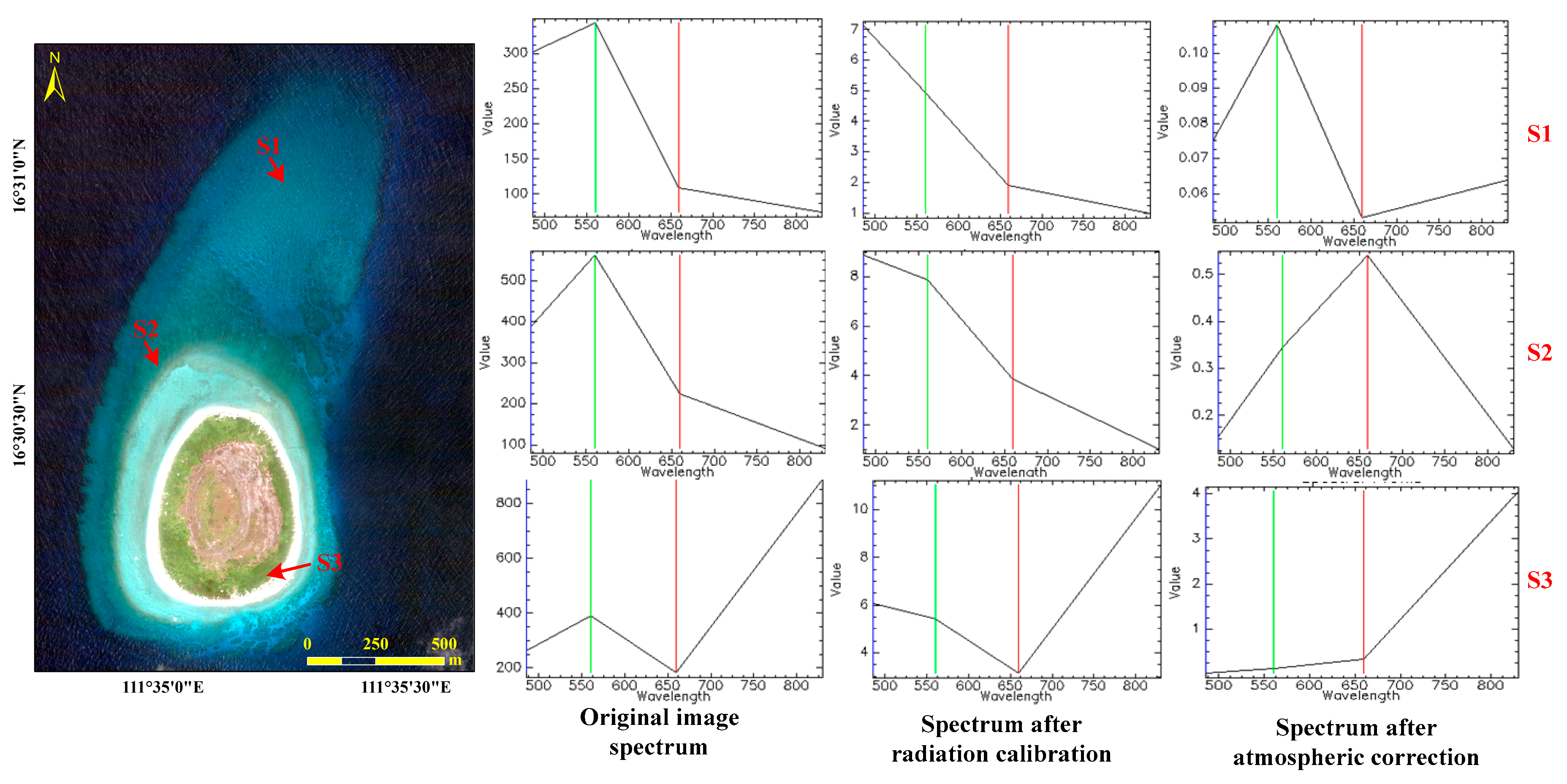
4.1. The Result of Radiation Calibration and Atmospheric Correction
The water body is the most important area after radiometric and atmospheric correction. Two sites at different depths of water and one site of vegetation were selected to observe the changes of the spectral curve after radiation calibration and atmospheric corrections, as shown in
Figure 7. Each row of spectral curves represents a site marked in the left image.
4.2. Comparison of Different Waveform Processing Means
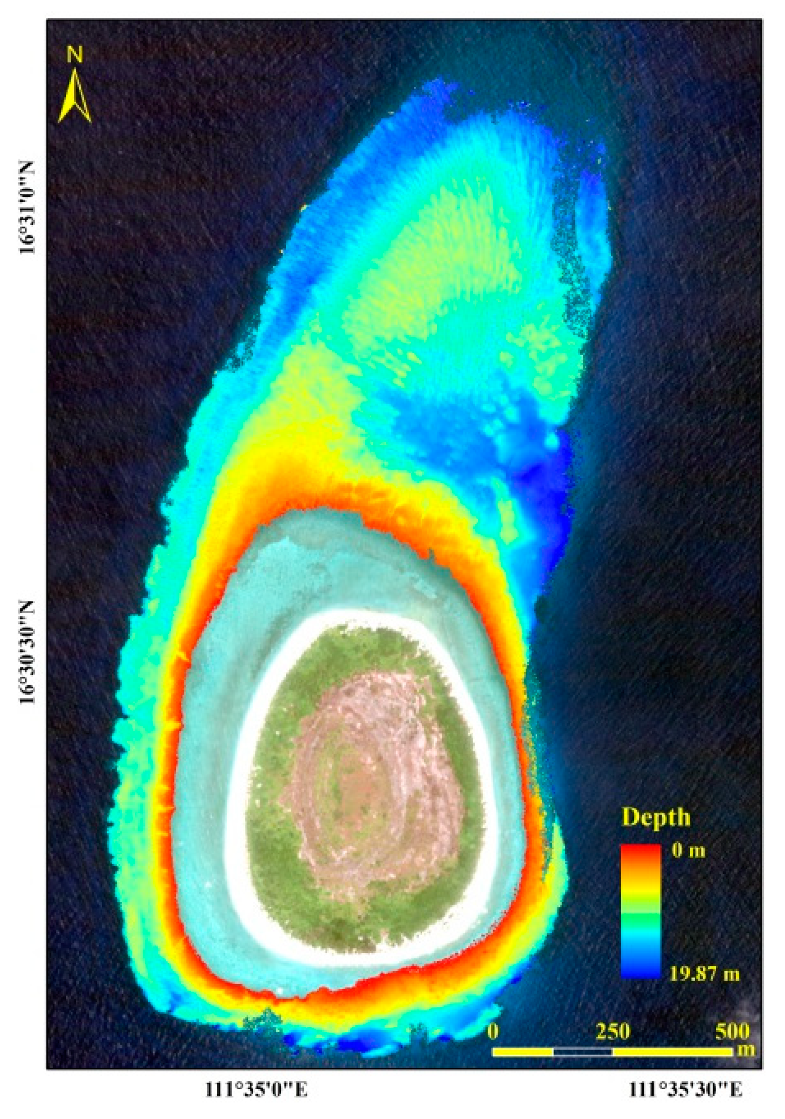
The LiDAR waveform data were fitted to extract the water depth using the multi-Gaussian function. The bathymetric map of the whole water area (
Figure 8) was obtained after tidal correction and data-level conversion.
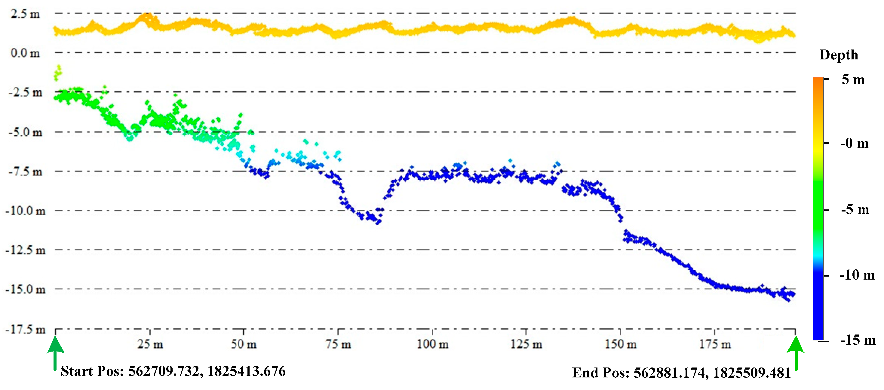
The water depth profile of northwest Ganquan Island is shown in
Figure 9. The horizontal coordinate represents the offshore distance, and the vertical coordinate represents the water depth value. In the figure, the yellow points represent the sea level, and the green and blue points represent water depth at different ranges. The slope gradient was gentle, and the depth changed slightly from 3 to 17 m.
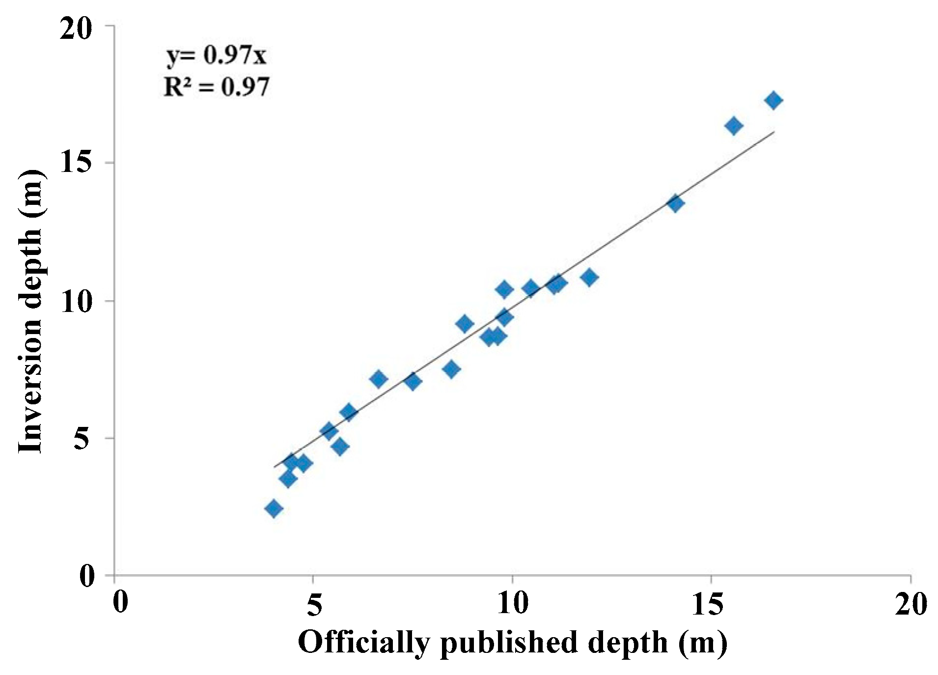
Validation points were selected from the profile at intervals of 10 m to quantify the relationship between the depth inversion result of the multi-Gaussian function and the officially published value by the LiDAR processing software. The scatter plot of the two depth values is shown in
Figure 10. The
R2 of the result of the multi-Gaussian function could reach 0.9 with an MRE of 5.6% in all water depth ranges. However, the MRE was relatively large in extremely shallow waters, and the time difference of the returning echo signals from the water surface and the bottom part was somewhat small and difficult to distinguish. The MAE of the whole water depth was 58.2 cm. When the water depth exceeded 15 m, the MAE became larger. This phenomenon may be due to the weak echo signal from the bottom part of the deep water that is difficult to identify.
4.3. Overall Accuracy of Inversion Result
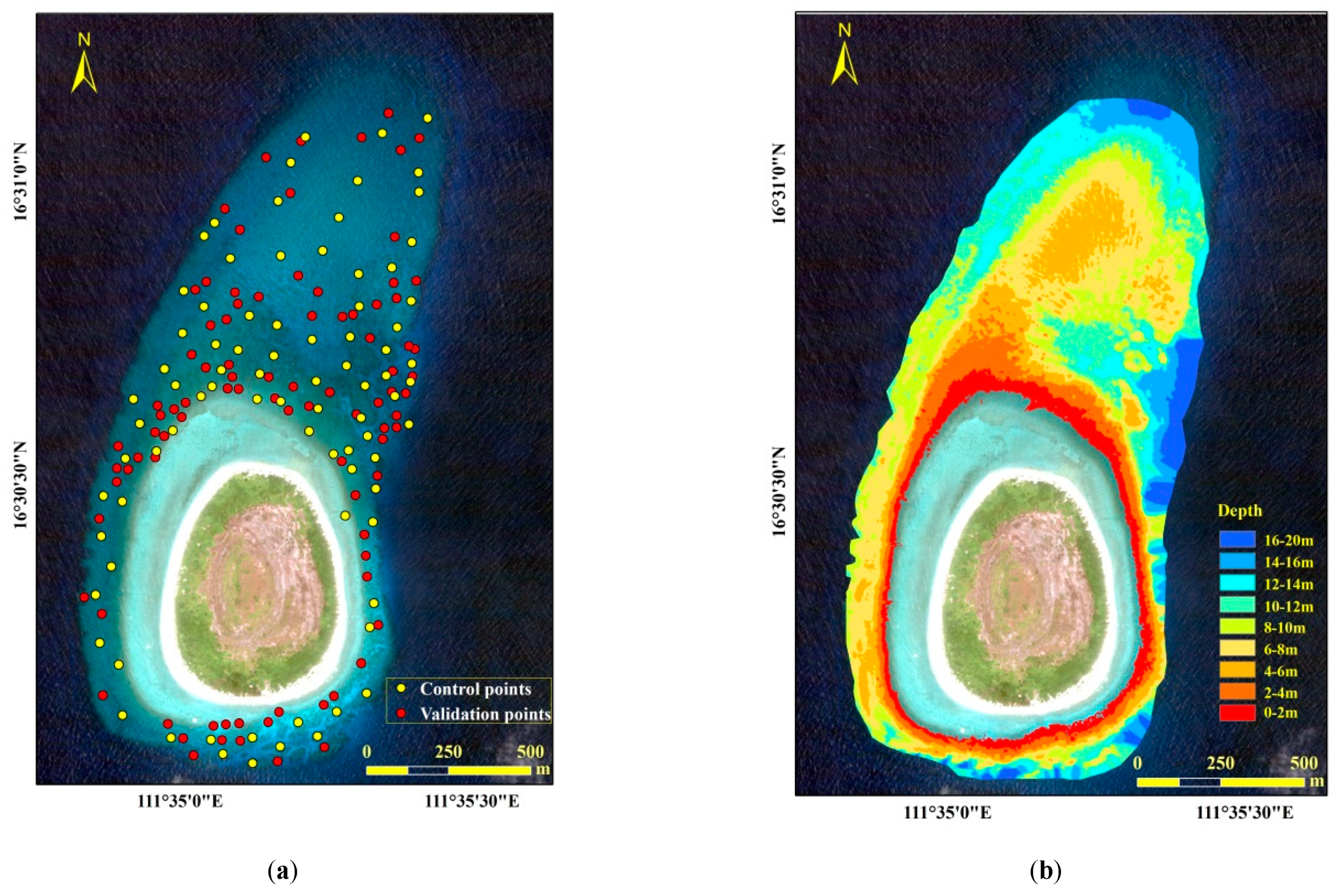
The data from the Aquarius LiDAR waveform were solved as survey data. A bathymetric inversion of the QuickBird image was carried out. Control and validation points were selected uniformly and randomly, and their numbers were 83 and 91, respectively. The distribution of the points is shown in
Figure 11a.
The regression relationship between the survey data and the inversion data of the control points was established with Equation (8). The Newton iteration method was applied to accomplish the regression of model parameters. The optimal regression parameters were
, and the
R2 of the fitting was 0.96. Control and validation points were then used with ILCRM to retrieve the depth value.
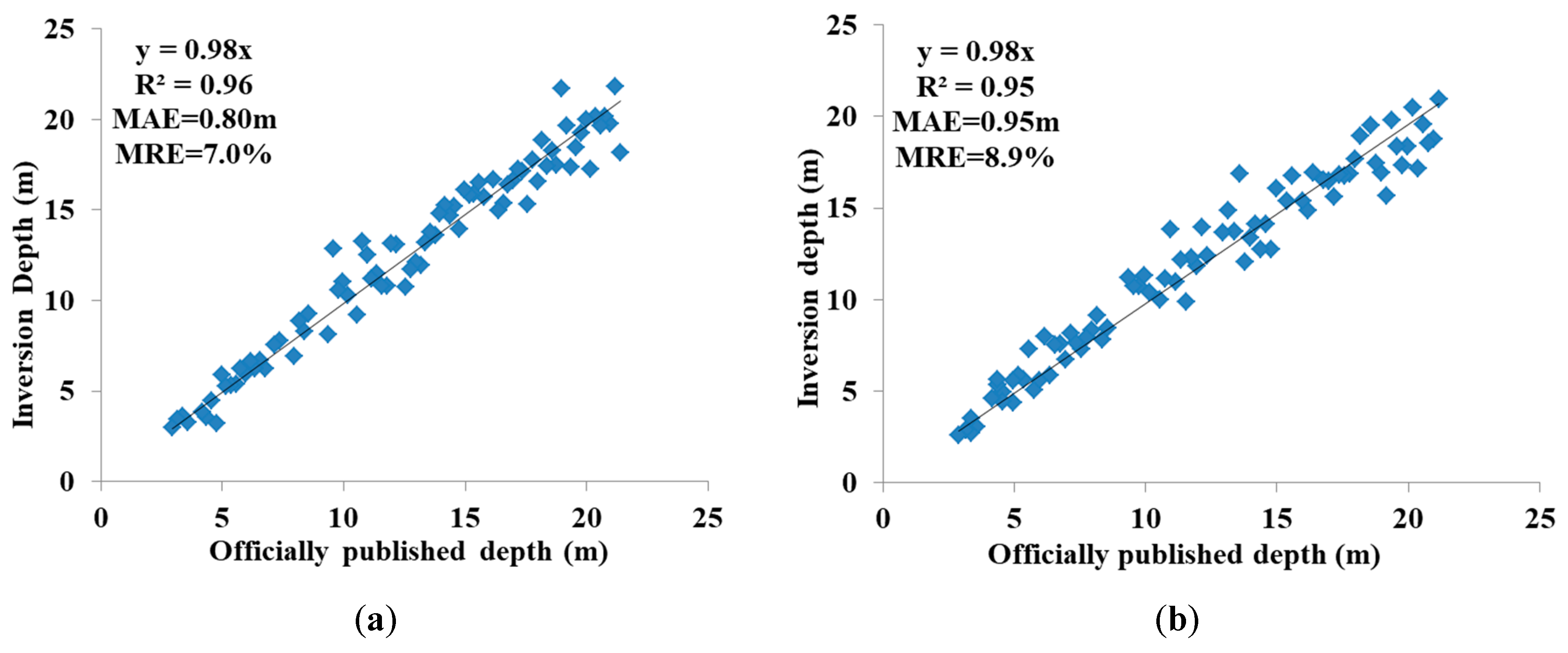
R2, MRE, and MAE were used as the evaluation indicators of accuracy. The overall accuracy of the inversion result is shown in
Figure 12.
Figure 11a,b show the scatter plots of the control points and the validation points, respectively. The derived depths of both points were well fitted with the survey data. However, the result of the validation points was more discrete than that of the control points, and the fitting coefficients of
R2 were 0.95 and 0.96, respectively. The water depth of the inversion was in the range of 2–22 m. The overall MAEs were 0.80 m and 0.95 m, and the overall MREs were 7.0% and 8.9%, respectively.
4.4. Accuracies of the Specific Depth Range
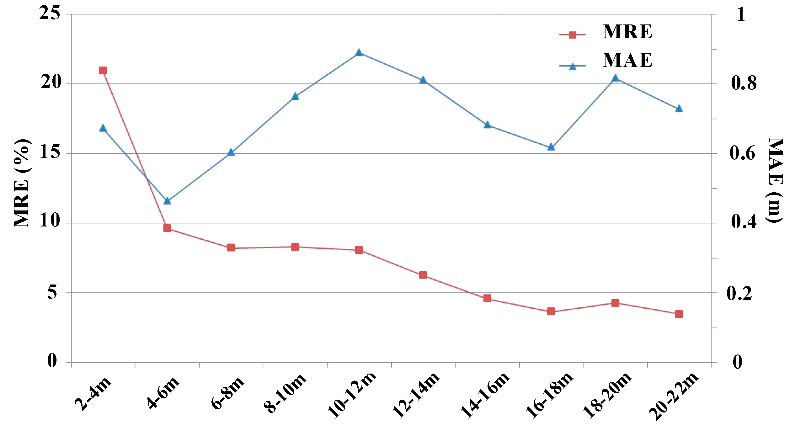
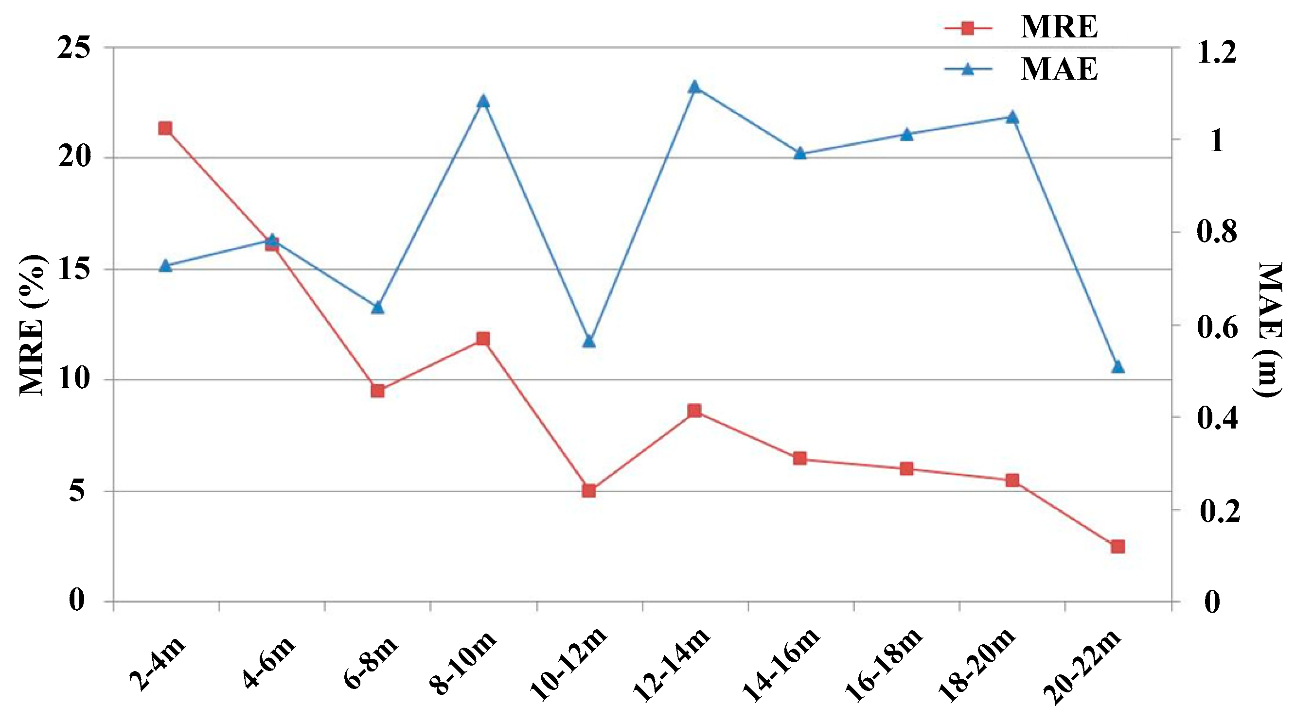
Water depth was divided into 10 ranges at the interval of 2 m to analyze the inversion ability of different specific depth ranges, namely, 2–4, 4–6, 6–8, 8–10, 10–12, 12–14, 14–16, 16–18, 18–20, and 20–22 m. MAE and MRE were used as the approximates of evaluation.
Figure 13 shows the MAEs and MREs of the specific depth ranges of the control points. The MRE of extremely shallow water (2–4 m) had the largest value. With the increase in depth, MRE tended to drop until it reached the minimum of 3.49% in the depth range of 20–22 m. The MAEs of all depth ranges were less than 0.9 m, and the dropping or rising tendencies were not obvious. The MAEs of 10–12 m and 4–6 m were the highest and lowest values at 0.89 m and 0.46 m, respectively.
Figure 14 shows the MAEs and MREs of the specific depth ranges of the validation points. With the increase in water depth, MRE appeared to be on a downward trend. The MRE of extremely shallow waters (2–4 m) was the highest at 21.32%. The differences in MREs of the much deeper waters (>14 m) were relatively small, and the MRE in the range of 20–22 m could reach the minimum value of 2.47%. The MAEs of all the depth ranges were within the range of 0.56–1.11 m, and dropping or rising tendencies were not obvious. The minimum and maximum MAEs appeared in ranges of 10–12 m and 12–14 m, respectively.
5. Discussion
Visible light is difficult to be quantitatively analyzed due to the variability and complexity of hydrological and atmospheric factors during their propagation. The improved band ratio algorithm, which is used to retrieve depth data from passive remote sensing, belongs to the classification of semi-analytical models. In this model classification, the detection capability of water depths is limited by the depth range of control points. Given that the control points provided by the Aquarius LiDAR data are in the range of 0–20 m, the derived bathymetry can be narrowed to a relatively small range.
The extraction of echo signals from extremely shallow waters and the bottom of deep waters has certain limitations. Further research is needed to identify and extract LiDAR waveform signals. The incident angle is a key parameter of bathymetric inversion. This study assumes that the incident angle for laser launching into waters is equal to the launch angle of the LiDAR. However, the assumption is inappropriate in complex sea conditions, and it needs to be gradually improved in later experiments.
6. Conclusions
On the one hand, bathymetry derived by LiDAR has the advantage of high maneuverability and efficiency, but the cost of using the system is high. On the other hand, the application of passive optical remote sensing entails poor accuracy, but the cost of using it is low. On the basis of the popularity of LiDAR bathymetry for depth measurements, bathymetric inversion with passive optical image became a research topic with high value. In this study, a multi-Gaussian function was used to fit the LiDAR waveform data, and the depth data were extracted for use as the measured depth data of bathymetric inversion. Then, the improved band ratio model was applied to estimate the bathymetry of the entire water around Ganquan Island within the QuickBird image range. The main conclusions are highlighted below.
On the basis of the multi-Gaussian function to fit the LiDAR waveform data, the overall MAE of the whole water depth (3–17 m) was 5.6%, the overall MRE was 58.2 cm, and the R2 could reach 0.97. The accuracies meet the requirements of ocean surveying and bathymetric mapping.
The bathymetric data derived from the Aquarius airborne LiDAR were divided into control points and validation points. On the basis of the improved band ratio model, a bathymetric inversion was carried out with the QuickBird image. The fitting coefficients R2 of validation points and control points were 0.95 and 0.96, respectively. In the range of 2–22 m, the overall MAEs were 0.80 m and 0.95 m, and the overall MREs were 7.0% and 8.9%, respectively. In specific depth ranges, the MAEs of all the depth ranges were within the range of 0.5–1.2 m. From the aspect of accuracy of both overall and specific depth ranges, the proposed method is an effective and inexpensive way to extract water depth information, given the combination of active and passive remote sensing. At the same time, costs can be reduced, indicating its applicability in coastal engineering in the future.
Suitable depth ranges need to be determined prior extracting the depth from LiDAR waveforms and combing active and passive remote sensing. Bathymetric inversion is limited in extremely shallow waters (<2 m) and deep waters. The difference in signals from the sea surface and the bottom in extremely shallow waters is somewhat small and, thus, difficult to distinguish, and the detection accuracy is low. By contrast, in deep waters, the signal from the bottom is too weak to be detected, thus resulting in poor accuracy.
Author Contributions
Conceptualization, Z.Z. and Y.M.; methodology, Z.Z. and T.J.; software, J.Z.; validation, Y.M., H.T., and T.J.; investigation, Y.M.; resources, Z.Z. and H.T.; Writing—Original Draft preparation, Z.Z.; Writing—Review and Editing, J.Z.
Funding
This research was funded by the Postgraduate Science and Technology Innovation Project of Shandong University of Science and Technology, grant number SDKDYC190204; the National Natural Science Foundation of China (NSFC), grant number 41706194; and the second remote sensing survey of East India Ocean environmental parameters, grant number GASI-02-IND-YGST2-04.
Conflicts of Interest
The authors declare no conflict of interest.
References
- Lyzenga, D.R.; Malinas, N.P.; Tanis, F.J. Multispectral bathymetry using a simple physically based algorithm. IEEE Trans. Geosci. Remote Sens. 2006, 44, 2251–2259. [Google Scholar] [CrossRef]
- Figueiredo, I.N.; Pinto, L.; Goncalves, G. A Modified Lyzenga’s Model for Multispectral Bathymetry Using Tikhonov Regularization. IEEE Geosci. Remote Sens. Lett. 2016, 13, 53–57. [Google Scholar] [CrossRef]
- Su, H.; Liu, H.; Wu, Q. Prediction of Water Depth from Multispectral Satellite Imagery—The Regression Kriging Alternative. IEEE Geosci. Remote Sens. Lett. 2015, 12, 2511–2515. [Google Scholar] [CrossRef]
- Tian, Z. Study of Bathymetry Inversion Models Using Multispectral or Hyperspectral Data and Bathyorographical Mapping Technology. Master’s Thesis, Shandong University of Science and Technology, Qingdao, China, 2015. [Google Scholar]
- Liang, J.; Zhang, J.; Ma, Y. spatial resolution effect analysis of remote sensing bathymetry. Acta Oceanol. Sin. 2017, 36, 106–113. [Google Scholar] [CrossRef]
- Wang, Y.; Zhang, P.; Dong, W. Study on Remote Sensing of Water Depths Based on BP Artificial Neural Network. Ocean Eng. 2007, 9, 568–571. [Google Scholar]
- Liang, Z.C.; Huang, W.Q.; Yang, Y. Study of the water depth retrieval based on artificial neural network. Eng. Surv. Mapp. 2012, 21, 17–21. [Google Scholar]
- Ma, Y.; Zhang, J.; Zhang, J.Y. Progress in Shallow Water Depth Mapping from Optical Remote Sensing. Adv. Mar. Sci. 2018, 36, 331–351. [Google Scholar]
- Wagner, W.; Ullrich, A.; Melzer, T. From Single-pulse to full-waveform airborne Laser Scanners: Potential and practical challenges. In Proceedings of the International Society for Photogrammetry and Remote Sensing 20th Congress Commission 3, Istanbul, Turkey, 12–23 July 2004; Volume 35, Part B/3. pp. 6–12. [Google Scholar]
- Wagner, W.; Roncat, A.; Melzer, T. Waveform analysis techniques in airborne laser scanning. Swiss Fed. Inst. Technol. Zürich 2007, 3, 602–605. [Google Scholar]
- Abdallah, H.; Baghdadi, N.; Bailly, J.S. Wa-LiD: A new lidar simulator for waters. IEEE Geosci. Remote Sens. Lett. 2012, 9, 744–748. [Google Scholar] [CrossRef]
- Abady, L.; Bailly, J.S.; Baghdadi, N. Assessment of Quadrilateral Fitting of the Water Column Contribution in Lidar Waveforms on Bathymetry Estimates. IEEE Geosci. Remote Sens. Lett. 2014, 11, 813–817. [Google Scholar] [CrossRef]
- Wang, D.L.; Xu, Q.; Xing, S. A Coarse-to-fine Signal Detection Method for Airborne LiDAR Bathymetry. Acta Geod. Cartogr. Sin. 2018, 47, 1148–1159. [Google Scholar]
- Jutzi, B.; Stilla, U. Range determination with waveform recording laser systems using a Wiener Filter. ISPRS J. Photogramm. Remote Sens. 2006, 61, 95–107. [Google Scholar] [CrossRef]
- Wu, J.; Van Aardt, J.A.N.; Asner, G.P. A Comparison of Signal Deconvolution Algorithms Based on Small-Footprint LiDAR Waveform Simulation. IEEE Trans. Geosci. Remote Sens. 2011, 49, 2402–2414. [Google Scholar] [CrossRef]
- Parrish, C.E.; Jeong, I.; Nowak, R.D. Empirical Comparison of Full-Waveform Lidar Algorithms. Photogramm. Eng. Remote Sens. 2011, 77, 825–838. [Google Scholar] [CrossRef]
- Billard, B.; Wilsen, P.J. Sea surface and depth detection in the WRELADS airborne depth sounder. Appl. Opt. 1986, 25, 2059. [Google Scholar] [CrossRef] [PubMed]
- Wong, H.; Antoniou, A. Characterization and decomposition of waveforms for LARSEN 500 airborne system. IEEE Trans. Geosci. Remote Sens. 1991, 29, 912–921. [Google Scholar] [CrossRef]
- Chen, W.B.; Lu, Y.T.; Chu, C.L. Analyses of Depth Accuracy for Airborne Laser Bathymetry. Chin. J. Lasers 2004, 31, 101–104. [Google Scholar]
- Yao, C.H.; Chen, W.B.; Zhang, H.G. Study of the Capability of Minimum Depth Using an Airborne Laser Bathymetry. Acta Opt. Sin. 2004, 24, 1406–1410. [Google Scholar]
- Zhang, Z.; Ma, Y.; Zhang, J.Y. Research on Depth of Water Detection Model Based on LiDAR Echo Signal of Simulation. J. Ocean Technol. 2015, 34, 13–18. [Google Scholar]
- Pacheco, A.; Horta, J.; Loureiro, C.; Ferreira, Ó. Retrieval of nearshore bathymetry from Landsat 8 images: A tool for coastal monitoring in shallow waters. Remote Sens. Environ. 2015, 159, 102–116. [Google Scholar] [CrossRef]
- Tian, Z.; Ma, Y.; Zhang, J.Y. Study on the Bathymetry Inversion by Active and Passive Remote Sensing with Landsat-8 Images and LiDAR Data. J. Ocean Technol. 2015, 2, 1–8. [Google Scholar]
- Tulldahl, H.M. Sea floor classification with satellite data and airborne lidar bathymetry. In Proceedings of the Ocean Sensing and Monitoring V., Baltimore, MD, USA, 3 June 2013; Volume 8724, p. 87240B. [Google Scholar] [CrossRef]
- Torres-Madronero, M.C.; Velez-Reyes, M.; Goodman, J.A. Subsurface unmixing for benthic habitat mapping using hyperspectral imagery and lidar-derived bathymetry. In Proceedings of the Algorithms and Technologies for Multispectral, Hyperspectral, and Ultraspectral Imagery XX, Baltimore, MD, USA, 13 June 2014; Velez-Reyes, M., Kruse, F.A., Eds.; SPIE: Baltimore, MD, USA, 2014; Volume 9088, p. 90880M. [Google Scholar] [CrossRef]
- Kerfoot, W.; Hobmeier, M.; Yousef, F.; Green, S.; Regis, R.; Brooks, C.; Reif, M. Light Detection and Ranging (LiDAR) and Multispectral Scanner (MSS) Studies Examine Coastal Environments Influenced by Mining. ISPRS Int. Geo-Inf. 2014, 3, 66–95. [Google Scholar] [CrossRef]
- Liu, J.; Wang, L.M.; Yang, L.B. GF-1 satellite image atmospheric correction based on 6S model and its effect. Trans. Chin. Soc. Agric. Eng. 2015, 19, 159–168. [Google Scholar]
- Lyzenga, D.R. Passive remote sensing techniques for mapping water depth and bottom features. Appl. Opt. 1978, 17, 379–383. [Google Scholar] [CrossRef] [PubMed]
- Lyzenga, D.R. Remote sensing of bottom reflectance and water attenuation parameters in shallow water using aircraft and Landsat data. Int. J. Remote Sens. 1981, 2, 71–82. [Google Scholar] [CrossRef]
- Philpot, W.D. Bathymetric mapping with passive multispectral imagery. Appl. Opt. 1989, 28, 1569–1578. [Google Scholar] [CrossRef] [PubMed]
- Chen, Q.D.; Deng, R.R.; Qin, Y. Water Depth Extraction from Remote Sensing Image in Feilaixia Reservoir. Acta Sci. Nat. Univ. Sunyatseni 2012, 51, 122–127. [Google Scholar]
- Tanis, F.J.; Byrne, H.J. Optimization of multispectral sensors for bathymetry applications. In Proceedings of the 19th International Symposium on Remote Sensing of Environment, Ann Arbor, MI, USA, 21–25 October 1985; pp. 865–874. [Google Scholar]
- Ji, W.; Civco, D.L.; Kennard, W.C. Satellite remote bathymetry: A new mechanism for modeling. Photogramm. Eng. Remote Sens. 1992, 58, 545–549. [Google Scholar]
- Benny, A.H.; Dawson, G.J. Satellite Imagery as an Aid to Bathymetric Charting in the Red Sea. Cartogr. J. 1983, 20, 5–16. [Google Scholar] [CrossRef]
- Di, K.C.; Ding, Q.; Chen, W. Shallow water depth extraction and chart production from TM images in Nansha islands and nearby sea. Remote Sens. Land Resour. 1999, 41, 59–64. [Google Scholar]
- Fu, J.; Gu, D.; Yang, H. A shallow water depth extraction model based on high resolution multispectral imagery. In Proceedings of the MIPPR 2009: Remote Sensing and GIS Data Processing and Other Applications, Yichang, China, 30 October 2009; p. 74982B. [Google Scholar] [CrossRef]
- Stumpf, R.P.; Holderied, K.; Mark, S. Determination of water depth with high-resolution satellite imagery over variable bottom types. Limnol. Oceanogr. 2003, 48, 547–556. [Google Scholar] [CrossRef]
- Bouhdaoui, A.; Bailly, J.-S.; Baghdadi, N.; Abady, L. Modeling the Water Bottom Geometry Effect on Peak Time Shifting in LiDAR Bathymetric Waveforms. IEEE Geosci. Remote Sens. Lett. 2014, 11, 1285–1289. [Google Scholar] [CrossRef]
- Wang, C.; Li, Q.; Liu, Y.; Wu, G.; Liu, P.; Ding, X. A comparison of waveform processing algorithms for single-wavelength LiDAR bathymetry. ISPRS J. Photogramm. Remote Sens. 2015, 101, 22–35. [Google Scholar] [CrossRef]
© 2019 by the authors. Licensee MDPI, Basel, Switzerland. This article is an open access article distributed under the terms and conditions of the Creative Commons Attribution (CC BY) license (http://creativecommons.org/licenses/by/4.0/).


