1. Introduction
Augmented Reality (AR) applications allow a user to interact with digital entities on top of a real environment [
1], often linking real objects to digital information. This linking process requires recognizing the semantics of an environment, a task which proves to be difficult. One solution to this problem is localization in digital twins. If the exact location of the device in the environment is known, then a digital twin can provide semantics to the environment. Determining this location is called localization or pose estimation. While systems such as GPS are able to provide a georeferenced location in outdoor environments, they are prone to errors in indoor environments, making them unusable as localization for many applications. Thus, indoor localization can be seen as a separate problem from outdoor localization. In
Section 2, we will discuss different existing approaches to global localization and their advantages and disadvantages.
Especially the Architecture, Engineering, and Construction (AEC) industry could profit from using augmented reality in areas yet to be digitalized. One such area is maintenance, where augmented reality can already be used for contextual data visualization and interactive collaboration [
2]. Worker efficiency could be increased by allowing direct access of an object’s digital twin through augmented reality. Data could be visualized directly on top of the real world, and changes or notes could be sent back to a central service immediately. Direct data availability could also improve the construction process itself. Comparing the as-is state to the as-should-be state of a construction site would be easier and faster, which in turn would uncover mistakes earlier. Applications in these areas would have to rely on localization to attribute data to its real world counterpart.
Global indoor localization requires digital information about the building a device is operated in, such as a digital twin. Digital building information is accumulated through a concept called Building Information Modeling (BIM) [
3]. BIM encapsulates geometry, structure, and semantics of a building over the whole building lifecycle. Over the years, BIM has seen a rise in popularity in the construction industries, and thus, the availability and sophistication of digital twins has improved. A more widespread use of digital building models would allow for more applications to procure detailed data directly from available sources, allowing for a direct connection between buildings and users. Therefore, BIM can benefit from a reliable localization as much as localization can be aided by using BIM data.
In this paper, we introduce a novel approach to localization in indoor spaces through the help of BIM. We aim for a computational, efficient 6 degrees of freedom (6-DOF) pose estimation algorithm that can accurately determine the position of an AR device in a known building. To achieve this, we use point clouds, BIM, and template matching.
3. Methodology
For this paper, we approach the localization problem with a floor-plan matching algorithm through template matching. Since point clouds provide a large amount of data, reducing the dimensionality of the data is key. The data is assumed to be in the form of point clouds, as much current hard- and software, e.g., SLAM algorithms and time-of-flight cameras, are able to generate point clouds from depth data. We also assume that the point-cloud data is accumulated over time. Of the incoming frames, every frame is processed into a point cloud. Through Inertial Measurement Units (IMUs) or SLAM, a transform between those frames can be established, linking each point cloud frame relative to each other. The 3D points from multiple frames can then be accumulated to a complete point cloud that includes observed geometry from all frames.
In our methodology, we take advantage of the nature of indoor environments, namely that indoor geometry is not arbitrary. Hallways and rooms are generally made up of straight walls, ceilings, and floors, which are usually perpendicular to each other. Walls are usually perpendicular to the floor and to each other, allowing us to make assumptions about unseen geometry. The most significant information about the layout of the observed environment is, therefore, found in the floor plan of the building. Floor-plan matching reduces the dimensionality of the problem. The position is determined along the x- and y-dimensions, disregarding the height of the pose. Of the rotational pitch, yaw, and roll, only the yaw of the pose can be calculated by floor-plan matching. The missing dimensions (height above floor level, pitch, and roll) can be easily determined by other sensors. The height above the floor level can be independently determined using a ground-plane estimation, which is often a standard feature in common AR frameworks. In our case, we will use a simple ground-estimation algorithm using normal filtering. Rotational pitch and roll can be found by using a device’s internal accelerometer, which even in common smartphone hardware is accurate to around 1° for inclination measures. Thus, we assume point clouds to be rotationally aligned with the ground plane. The algorithm is, therefore, able to break down the 6-DOF pose estimation into 3-DOF localization including orientation.
The aim is to find a proper rigid transformation T between the local coordinate system of the AR device and the world coordinate system of a given building model. As the input data, only collected point-cloud data and local position changes of the device are to be used. Finding the transformation should be done in a time-efficient manner so that the localization of the AR device can be done in real time. Matching the update speed of the device is not required, as the device can use existing inertial sensors to track its location between updates of the transformation. The local transformation from the inertial sensors are able to keep the device responsive between updates, allowing the system to keep the necessary responsiveness and interaction required for AR. Run times in the area of milliseconds to a few seconds are, therefore, acceptable. An augmented reality system could request a new transform every few seconds to correct its local transform. The system can use the provided transform between the local coordinate frame and the BIM model coordinate frame to match its surrounding environment to the BIM model. The algorithm’s targeted accuracy depends on the applied task. Indoor navigation requires an accuracy of about 1 m, while contextual information displays require to be accurate to a few centimeters.
The proposed algorithm is based on two-dimensional template matching of recorded floor plans onto existing building models. The given BIM model of a building is transformed into a 2D distance map for template matching against a processed point cloud. For a recorded point cloud, we determine several possible rotation candidates around the
z-axis. Since it is assumed that the point cloud is rotationally aligned with the ground through accelerometers, only one rotational degree of freedom has to be solved. For the set of rotations, we calculate a transformation over the
XY plane using template matching of floor plans.
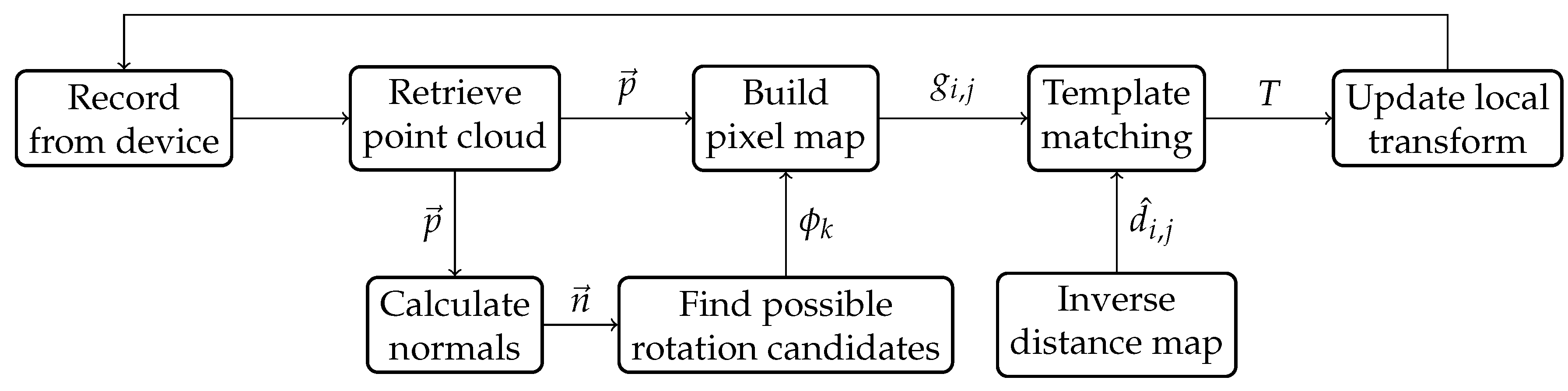
Figure 1 gives an overview of the localization steps. In
Section 3.5, we will introduce methods for improving run-time efficiency by caching and updating parts of the matched templates over time.
3.1. BIM Distance Map
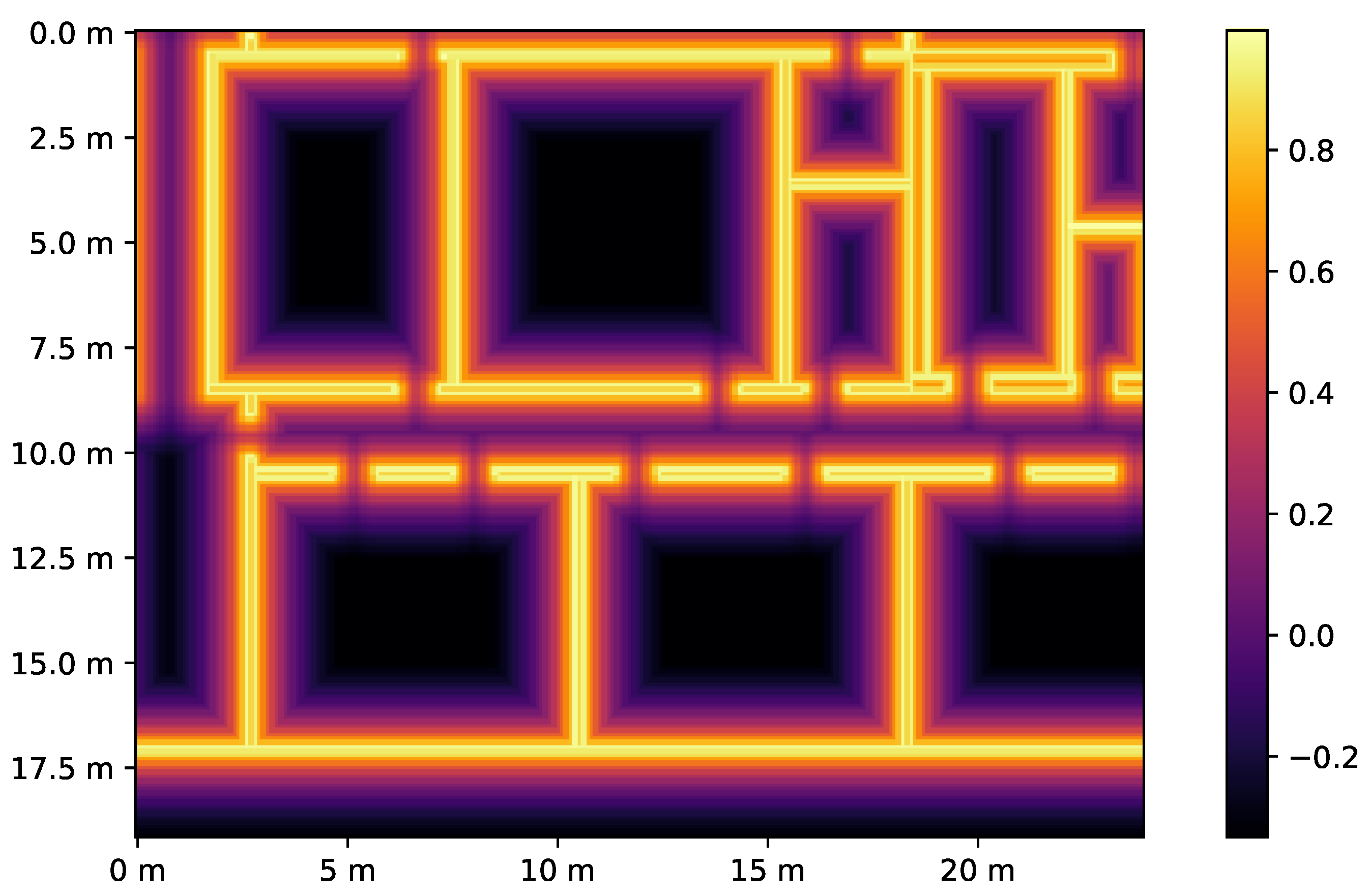
To prepare a BIM model for localization, the 3D model has to be transformed into a 2D map for template matching. For every floor of the BIM model, we set a cross section over the XY plane, which is the basis of the template-matching map. The cross section is placed at roughly the same height as a device would be held above floor level. Since point-cloud data gathered from depth sensors is inherently noisy and the environment may be obstructed by furniture, the recorded point cloud will differ from the original BIM model. These spatial inaccuracies are not accounted for template matching against a binary map representation of the BIM model. An error of 10 cm would have the same negative impact on the correlation as an error of 1 m. Therefore, we match against the inverse distance map of the BIM model. The inverse distance map allows for correction of small errors in the point cloud when template matching while still penalizing inaccuracy. The distance map for the model can also be calculated and cached beforehand and has no impact on efficiency.
To calculate the inverse distance map, every cell position of the distance map is assigned a 3D coordinate on the cross section of the floor. For every cell position
, we find the closest point on a wall
. The distance to the closest wall equals
for every cell. We then calculate the inverse distance map over all pixels
:
which results in higher values the closer the position
is to a wall.
Figure 2 shows an example of the inverse distance map. The closer a pixel on the template is to a wall, the higher the correlation value. Large environments may require a cutoff distance to avoid penalizing inconsistently as the center of a room would be penalizing outliers much more harshly than other places.
3.2. Finding Rotation Candidates
When a point-cloud frame is recorded, it is processed for template matching. To keep the template-matching run time to a minimum, only a few possible rotations for the point cloud are considered. We therefore determine a set of rotation candidates that are most likely to match the recorded point cloud with the BIM model. Using the knowledge of our domain, we can assume that the walls recorded in the point cloud must face the same direction as the walls in the reference model. We use a convolution of normals in Fourier space to find the best rotational candidates. The rotation candidates are determined as follows:
Calculate normals for the point cloud using a normal estimation algorithm. All normal vectors are assumed to be unit vectors.
Project every normal vector onto the XY plane.
Transform the projected vector from a two-dimensional coordinate system to a polar coordinate system, which yields a rotation and magnitude for every normal vector.
Filter out vectors by magnitude. Vectors with a magnitude below a certain threshold can be ignored, as they are most likely situated on a floor or ceiling of the point cloud.
Generate a histogram based on the rotation of the vectors. This histogram requires a form of binning.
Compute a convolution between the histogram of normal rotations and a target wave, and determine the best fit. The target wave has to match the general directions of walls in the reference model. A reference model with only perpendicular walls would yield four rotational candidates after a convolution with a sine wave . Since the histogram is binned, the convolution can be calculated efficiently by transforming the histogram into Fourier space using a discrete fast Fourier transform algorithm.
The maximum value of the convolution is the optimal rotation of the point cloud to the reference. Additional rotation candidates can be calculated by adding (in the case of perpendicular walls) 90 °, 180 °, and 270° to . Depending on the geometry of the building, more rotational candidates may be defined.
3.3. 2D Rasterization
To enable template matching of the point cloud, the point-cloud representation needs to be transformed into a two-dimensional map for every rotational candidate. After applying the rotation to the point cloud, a grid
g over the
XY plane is created with resolution
r. Each pixel on the resulting image represents the number of points contained within a grid cell.
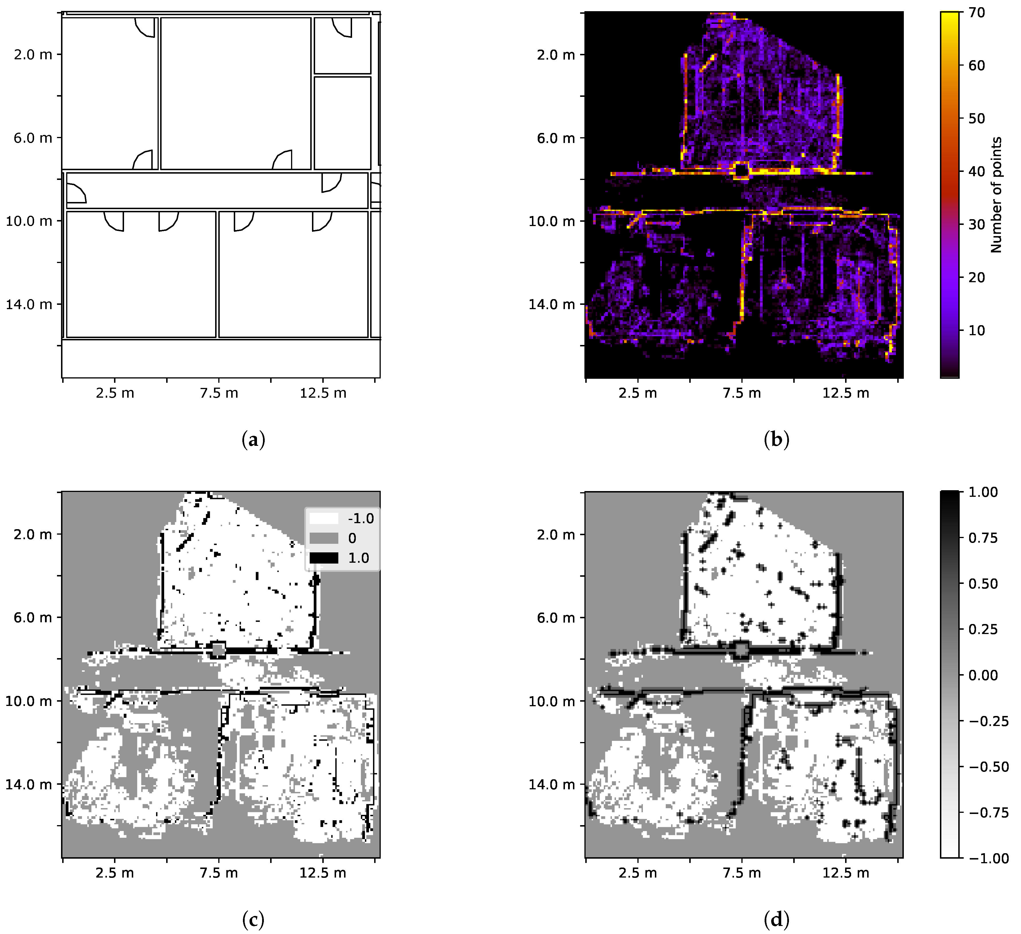
Figure 3a shows a floor plan of the BIM model, and
Figure 3b shows a corresponding recorded point cloud. The resulting image is then split into three categories:
Wall,
Floor, and
No Observation. This is done through thresholding, where each category is assigned a value of 0, greater than 0, and lower than 0:
The pixel map
contains the number of points of which the
coordinates correspond to the grid cell
. The values
and
are the thresholds of vertices needed in a cell to be recognized as a wall or floor, respectively. In the resulting image, a wall pixel has a positive value; a floor pixel a negative value; and when no observation has been made, the pixel is set to 0, as seen in
Figure 3c. The parameter
β ∈ [0,1] balances floor and wall pixels, giving higher importance to either observed floors or walls. During template matching, walls in the point cloud correlate positively with walls in the model while floors in the point cloud correlate negatively with walls in the model. Cells in which the point cloud shows no observation are set to zero and have no impact on the template matching. This rewards correct matching of walls while punishes missing walls where an observation has been made.
To improve wall matching, we also perform binary dilation on all wall pixels. This dilation creates a fast approximation of the distance calculation done in
Section 3.1, improving robustness. The distance
in pixel of the dilation should roughly match the distance cutoff of the inverse distance map. Without the dilation, large empty spaces would be treated favorably as the amount of wall pixels to floor pixels differs. The dilation is then added to the grid map, resulting in the final grid map as the weighted sum of both maps:
The factor
α weighs the two maps and should be between 0 and 1.
Figure 3d shows an example of a grid map
g.
3.4. Template Matching
With the inverse distance map
and the rasterized point cloud
of the floor plan obtained, we try to find the best positional match for the point cloud in the BIM model. For the template matching, we perform a convolution to find the best match for the localization. The convolution is defined as follows:
The convolution is performed for every rotational candidate. The maximum value of over all rotational candidates yields the localized position and the rotation , which is the most likely transformation T of the point cloud.
3.5. Template Caching
The introduced algorithm uses the whole point cloud for each localization pass, but between localization passes, only parts of the point cloud are changed as the environment is observed. Sections of the point cloud that are not observed in an update step are also left unchanged. Since convolutions are expensive, we can take advantage of caching to improve performance. We split up the rasterized grid
g from
Section 3.3 into multiple two-dimensional blocks
, such that we have the following:
Since the convolution is distributive, we can compute the convolution of the template matching step for every block individually and sum up the results:
This allows us to only recalculate convolutions in areas which have been updated in the last step. When the recorded point cloud increases in size, the computation time of the convolution, thus, stays unaffected.
3.6. Ground Estimation
In the case of matching point clouds of a single floor, a simple ground estimation will suffice for this application. Along the
z-axis, points cluster at the floor and ceiling levels. When filtering out points with downward-facing normals, only clusters on the floor are left. The
z values of the points are then divided into bins along the axis. The bin with the most points can be established as the ground plane with height
. The final transformation
T can then be calculated:
4. Evaluation
To test the accuracy and reliability of the algorithm, we have recorded point-cloud data and pose data using Microsoft HoloLens. Our reference model is a BIM model of a university building, where we match on a 3000 m
2 floor space. The model has multiple self-similar rooms and hallways to test reliability.
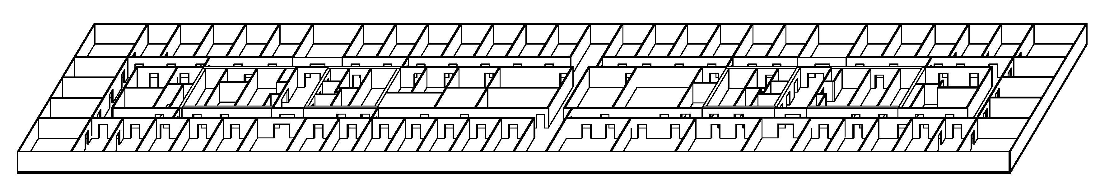
Figure 4 shows the floor plan of the BIM model used for localization.
4.1. Testing Scenarios
We used Microsoft HoloLens to record point clouds in three different locations in the building. The recorded point clouds cover a number of possible scenarios.
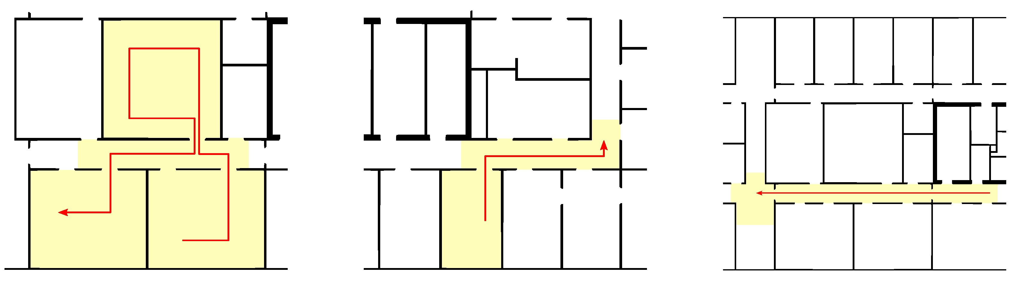
Figure 5 shows the three scenarios including the total recorded area in square meters and the walked path. For every scenario, we recorded 20 frames of point-cloud data. The frames were recorded evenly spaced (about 1 m apart) along the walked path. To determine the ground truth, the recorded point-cloud frames have been aligned manually with a ground truth pose
. The following scenarios have been recorded:
Scenario S1: The device starts in one room, moves out into the hallway, enters another room, turns back into the hallway, and enters a third room (see
Figure 5a). The rooms in this scenario are distinct from other rooms in the building model. This scenario tests the accuracy when moving through multiple different rooms. The walked path has a total length of 21.02 m, and the point cloud frames cover a total area of 169.41 m
2.
Scenario S2: The device starts in a single room, exits into the hallway, and moves around a corner (see
Figure 5b). Many rooms in the given building model are self similar and can be confused for other rooms. The walked path is 18.65 m in length with 62.45 m
2 of area covered.
Scenario S3: The device moves down a single hallway up until an intersection (see
Figure 5c). Straight hallways are often difficult for localization algorithms, as they can be visually indistinguishable at different positions. The path has a length of 24.29 m, and the hallway has an area of 57.94 m
2.
The grid size of the rasterization has been set to 10 cm. The parameters for thresholding have been set to and , which depend on the chosen spatial resolution of the HoloLens. To optimize the results, we used a grid search over the recorded data to determine the factors and .
Each point cloud frame is fed into the algorithm, resulting in an estimated pose
T. We then calculate the positional and rotational difference
and Δ
ϕ as a way of measuring localization accuracy. We categorize a localization as correct if
is smaller than 0.5 m and Δ
ϕ is smaller than 5°.
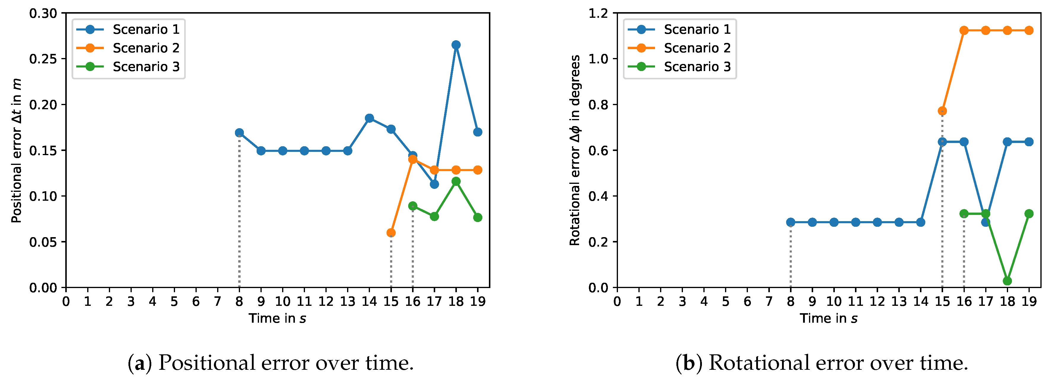
Figure 6 shows the localization error of correctly localized frames. The average error over all correctly localized point clouds is about 10–20 cm over the
xy plane and 1 cm and 5 cm for the ground estimation. Localization errors for incorrect localizations are between 10 m and 100 m. No localization errors between 1 m and 10 m were observed. This gap can be explained as the algorithm mistaking the observed area as a room in a different part of the building. Since rooms are about 10 m in size, localization errors in between are unlikely.
The reliability is measured through the point of first correct localization. At this point, the localization error is smaller than 0.5 m and 5°.
Table 1 shows the time, distance, and covered area of the first successful localization of each scenario. Notable is that, once the localization is correct, the localization stays correct for the remainder of the scenario.
4.1.1. Scenario S1
In this scenario, we examine localization accuracy in a non-self-similar environment. The second room to be visited is distinct in its dimensions from other rooms. Thus, the first correct localization can be observed in frame 8, when the first room has been completely observed and the second room has been observed halfway.
Figure 6 shows that the accuracy of localization is below 30 cm and 1°. The average translational error for correctly localized poses is 16.3 cm, and the average rotational error is 0.402°. The ground estimation has an average error of 4 cm, the highest of the three scenarios, which correlates with the area covered. The best accuracy in this scenario can be found when the device first observes the second room. After this, the localization accuracy decreases again, which points to inaccuracies of the device accumulating over time. Older point-cloud data may become shifted due to accumulative errors in the device’s internal tracking systems.
4.1.2. Scenario S2
Scenario S2 starts in a room that is self similar to multiple other rooms in the building. After recording the room, the device is moved outside. When only the room and the adjacent hallway are observed, localization is inconclusive. The guessed position jumps all over as similar-sized rooms can be found through the building. After walking about 14 m, the device observes the corner of the hallway. At this frame, the point cloud is sufficiently distinct and the localization can determine the position with an accuracy of 12 cm and 1°. This scenario shows that self similarities can be mitigated by an increased observed area. The surrounding geometry must be distinguishable from similar environments to give a reliable localization result.
4.1.3. Scenario S3
Scenario S3 shows the localization of a hallway, a structure that can be found at multiple different locations in the building. Similar to Scenario S2, the localization is unreliable until the geometry is sufficiently distinct. During movement, the point cloud is matched to multiple different hallways, as there is not enough information about the hallway for a correct localization. Only when the intersection is reached can the localization accurately match the position with a 9 cm error. Rotational error is the lowest in this scenario at 0.25°.
4.2. Results
As seen in all three scenarios, reliability suffers in self-similar environments. A point must be reached where the geometry of an environment is sufficiently different from other poses. Only then can the localization be reliable, as the localization remains correct after the first correctly guessed pose. In our scenarios, the user had to move the device 15–20 m until a reliable pose could be estimated. The area covered is also related to reliability as first correct localizations were observed from 50–110 m2. The reliability, thus, depends strongly on the geometry of the building one tries to localize in as well as on the amount and type of environment observed. Especially buildings with multiple self-similar floors would suffer from reliability problems. The more distinct geometry is observed the higher the reliability gets.
If localization is successful, the accuracy is in the range of 5–30 cm to a manually aligned point cloud. This difference can be attributed to inaccuracies during measurement as well as to drifts during recording caused by the device IMU. The naive ground estimation has an accuracy below 5 cm. Due to the rasterization process, the accuracy is bound by the rasterization grid size. A finer grid may improve localization but will decrease performance. This offers a trade-off between accuracy and performance.
The performance of the algorithm is acceptable. On a computer with 4 cores at 3.7GHz, a localization procedure of the tested scenarios takes less than 100 ms. On the HoloLens itself, the procedure takes about 500–1000 cm. This allows the localization to be considered in real time, as positioning in between localization frames can be handled by existing IMU systems. Since the procedure is highly parallelizable, it is scalable for future hardware. Thus, development in hardware will improve algorithm performance.
5. Conclusions
The proposed algorithm provides a novel way of performing pose estimation of an augmented reality device in a digital twin. The digital twin is obtained through existing BIM models, allowing localization in all buildings which provide such a model. We break the problem of pose estimation down from a 6-DOF problem into multiple independent dimensions. Two rotational degrees of freedom are obtained by hardware sensors, the height above ground is calculated using a ground-plane estimation, and the position in the building is determined by template matching. The input for our algorithm is point-cloud data and sensor information from AR hardware, making the approach independent of external sensors.
Our algorithm achieves higher accuracy than current vision-based approaches such as BIM–PoseNet [
19], which is around 2 m, and requires no extensive training phase. While Boniardi et al. [
23] achieve a higher accuracy and reliability, the approach requires knowledge about the initial position of the device. The UAV localization presented by Desrochers et al. [
14] has a similar accuracy to our algorithm but requires a significantly longer computation time on similar-sized environments, making it not applicable for AR localization. In our algorithm, aligning the recorded point cloud through normal analysis allows for a significant reduction in computation time and applying template matching on floor plans ensures a high accuracy with good performance. Performance of the algorithm proves to be in line with modern AR hardware capabilities, which allows for localization even when no network connection is available. Scalability of the algorithm can be a problem, since complexity scales with the size of the digital twin and the observed environment. Still, the performance impact of the observed environment can be alleviated by using template caching.
The accuracy performs well over all environment sizes and improves with more observed environments. Large localization errors occur in most part when not enough of the environment is observed and may offer widely inaccurate results. This could be mitigated by introducing a certainty value which could inform a user that more information about the environment is necessary for a localization. Since the localization may drift over time, a value for point age could be introduced. Older observations could be weighted less favorably than new observations or be removed from the point cloud entirely. This would allow for dismission of mistakes made by the device’s local positioning systems. Self similarities are still a problem for the proposed algorithm, but since all the previously observed environments are considered for localization, we achieve better results in self-similar environments than stateless image-based methods. Accuracy in self-similar environments could be improved by introducing sensor fusion. If external beacons such as Wi-Fi signals are used to narrow in on the correct location, self similarities over multiple floors and reflections could be reduced. Utilizing the semantics of the surroundings may also improve localization, e.g., recognizing certain structures such as doors or windows or recognizing signage.
Our approach shows that floor-plan matching is an appropriate approach for AR localization. With the proposed algorithm, it is possible to compute a mapping between the local device coordinates and the BIM model. From the 2D mapping, the position of the device can be determined to about 10 cm and 1° after exploring the surrounding geometry sufficiently. This exploration phase may require the user to walk 15–20 m, which may depend on the amount of self similarity inherent to the building.
Maintenance workers may benefit from an augmented reality room-layout display with data provided by BIM models or databases. Since reliability can only be assured when enough distinct geometry has been observed, a user would have to explore the space around them before they are correctly localized. This is easily achievable in the case of maintenance work, where multiple locations are likely to be visited. If the device is switched on as soon as the building or floor has been entered, the localization will be reliable by the time a maintenance location has been reached. Especially when using a head-mounted device, the localization can keep observing the surrounding space without interfering with work or requiring special attention. A maintenance worker could then be offered information about the room they are in, could see contextual displays for devices that are at a static location in the building, or could visualize structures hidden behind walls and floors [
2,
5].
Another possible application for this research is indoor navigation for AR devices. With the mapping between the BIM model and the device coordinate frame, the location of the device in the building can easily be determined and a path to a goal can be calculated by using standard navigation algorithms. To mitigate the requirement of observing sufficiently different geometry, improvements to reliability can be made by including more of the available data of an AR device. External sensors as a secondary source of information may further help against self similarities and computer vision as they can be optionally installed in a building. Learning techniques could improve the knowledge of a building over time and could correct repeated mistakes. Thus, if combined further with other approaches, localization could be made fast, accurate, and reliable.


