Article

Selective Finite Memory Structure Filtering Using the Chi-Square Test Statistic for Temporarily Uncertain Systems

Department of Electronic Engineering, Korea Polytechnic University, Siheung-si, Gyeonggi-do 15073, Korea
Appl. Sci. 2019, 9(20), 4257; https://doi.org/10.3390/app9204257
Submission received: 9 September 2019 / Revised: 2 October 2019 / Accepted: 7 October 2019 / Published: 11 October 2019
(This article belongs to the Section Mechanical Engineering)

Abstract

:

Featured Application

The current work might be appropriate for fast detection and identification of unknown signals whose time of occurrence cannot be predicted, which can arise from diverse engineering problems such as fault detection and diagnosis of dynamic systems, maneuver detection and tracking of moving objects, etc.

Abstract

In this paper, a finite memory structure (FMS) filtering with two kinds of measurement windows is proposed using the chi-square test statistic to cover nominal systems as well as temporarily uncertain systems. First, the simple matrix form for the FMS filter is developed from the conditional density of the current state given finite past measurements. Then, one of the two FMS filters, the primary FMS filter or the secondary FMS filter, with different measurement windows is operated selectively according to the presence or absence of uncertainty, to obtain a valid estimate. The primary FMS filter is selected for the nominal system and the secondary FMS filter is selected for the temporarily uncertain system, respectively. A declaration rule is defined to indicate the presence or absence of uncertainty, operate the suitable one from two filters, and then obtain the valid filtered estimate. A test variable for the declaration rule is developed using a chi-square test statistic from the estimation error and compared to a precomputed threshold. In order to verify the proposed selective FMS filtering and compare with the existing FMS filter and the infinite memory structure (IMS) filter, computer simulations are performed for a selection of dynamic systems including a F404 gas turbine aircraft engine and an electric motor. Simulation results confirm that the proposed selective FMS filtering works well for nominal systems as well as temporarily uncertain systems. In addition, the proposed selective FMS filtering is shown to be remarkably better than the IMS filtering for the temporarily uncertain system.

1. Introduction

Feature selection is known as one of core concepts in the field of machine learning based fault diagnosis [1,2,3]. There are several feature selection approaches available such as information gain, mutual information, and the chi-square test [4,5,6]. Among them, the chi-square, also written as χ 2 , test statistic can be also used for abnormal signal detection [7,8]. The chi-square test statistic is developed from the difference between two variables such as the original state and its filtered estimate, and then compared with a precomputed threshold to detect abnormal signals.
Meanwhile, in contrast to the recursive infinite memory structure (IMS) filter like the traditionally used Kalman filter [9,10,11,12], the finite memory structure (FMS) filter has been known to have inherent good properties such as bounded-input, bounded-output (BIBO) stability and and more robustness against temporary uncertainties due to its processing manner of finite measurements on the most recent window [13,14,15,16]. Thus, the FMS filter has been applied successfully for various engineering problems [17,18,19,20,21,22,23]. As shown in [13,14,15,16], the FMS filter is known to have better noise suppression as the measurement window length grows. In other words, the noise suppression of the FMS filter is closely related to the measurement window length. However, even if the FMS filter can show greater noise suppression as the window length increases, the tracking speed of the state estimate for the actual state variable worsens in proportion to the window length, which can degrade the estimation performance of the FMS filter. This implies the FMS filter requires a compromise between the noise suppression and the tracking speed of the state estimate. According to this observation, the estimation error of the FMS filter with a short measurement window length is smaller than that of the FMS filter with a long measurement window length, while uncertainty exists. In addition, the convergence of the estimation error for the FMS filter with a short window length is much faster than that of the FMS filter with a long window length when temporary uncertainty is disappearing. This means that the FMS filter with a short window length is superior in terms of the tracking ability. Thus, if the FMS filter with a short window length is applied to temporarily uncertain systems, it can outperform the FMS filter with a long window length, although the FMS filter with a short window length is designed without considering the robustness.
This paper proposes an FMS filtering with two kinds of measurement windows using the chi-square test statistic to cover the nominal system as well as the temporarily uncertain system. The simple matrix form for the FMS filter is developed from the conditional density of the current state given finite past measurements. Then, one of the two FMS filters, the primary FMS filter and the secondary FMS filter, with different measurement windows is operated selectively to obtain the valid estimate according to presence or absence of uncertainty. The primary FMS filter is selected for the nominal system and the secondary FMS filter is selected for the temporarily uncertain system, respectively. A declaration rule is defined to indicate the presence or absence of uncertainty, operate the suitable one from two filters, and then obtain the valid filtered estimate. A test variable for the declaration rule is developed using a chi-square test statistic from the estimation error and compared with a precomputed threshold. Finally, computer simulations are performed for a two kinds of dynamic systems such as a F404 gas turbine aircraft engine and electric motor to verify the proposed selective FMS filtering with two kinds of measurement windows and compare with existing FMS filtering and IMS filtering. Through computer simulation works, it is confirmed that the proposed selective FMS filtering works well for the nominal system as well as the temporarily uncertain system. It is also shown that the proposed selective FMS filtering can be remarkably better than the IMS filtering for the temporarily uncertain system.
This paper is organized as follows. In Section 2, the FMS filter is introduced. In Section 3, the selective FMS filtering with two kinds of measurement windows is proposed. In Section 4, computer simulations are performed. Finally, conclusions are presented in Section 5.

2. Finite Memory Structure Filter from the Conditional Density of the Current State Given Finite Measurements

As shown in [9,10,11,12,13,14,15,16,17,18,19,20,21,22,23], the state-space approach has been a general method for modeling, analyzing and designing a wide range of control and estimation problems in diverse dynamic systems, and has been especially suitable for digital computation techniques. Therefore, in this paper, a general discrete-time state space model with noises is considered as follows:
x i + 1 = A x i + G w i ,
z i = C x i + v i ,
where x i n is the unknown state vector of the state variables and z i q is the sensor measurement vector of the output variables. The state vector x i consists of n state variables and describes a dynamic system by a set of first-order difference equations with the state transition matrix A. A description of the dynamic system in terms of a set of state variables does not necessarily include all of the variables of direct engineering interest. Therefore, the sensor measurement vector z i is defined to be any system variable of interest using the output matrix C. Thus, the state transition matrix A is the property of the dynamic system and is determined by the system structure and elements. The output matrix C is determined by the particular choice of output variables. For example, in the electric motor system that will be covered in computer simulations, the state vector x i consists of two state variables such as armature current and rotational speed. The state transition matrix A contains physical elements such as armature resistance, armature inductance, motor inertial coefficient, etc. The sensor measurement vector z i is defined with the output matrix C to be the rotational speed that measured by corresponding sensor. The state vector x i 0 at the initial time i 0 of system is a random variable with a mean x ¯ i 0 and a covariance P i 0 . A dynamic system can often contains noises such as the system noise w i p and the measurement noise v i q . These noises are random variables with zero-mean white Gaussian and are mutually uncorrelated. In addition, these noises are also uncorrelated with the initial state vector x i 0 . The covariances of noises w i and v i are denoted by Q and R, respectively and they are assumed to be positive definite matrices. Since these noises can cause system performance degradation, the system output, i.e., the rotational speed in the electric motor system, should be corrected using the state estimation filtering.
To overcome shortcomings of the IMS filter like the traditionally used Kalman filter, the FMS filter has been developed by combining the Kalman filter with the moving window strategy [13,14,15,16]. The window of finite measurements moves forward with each sampling time when a new measurement is available from sensors. In other words, the FMS filter utilizes only the finite number of measurements on the most recent filtering window while discarding past measurements outside the filtering window.
The FMS filter, denoted by x ^ i at the current time i, is developed using the finite number of measurements, denoted by Z M . From the discrete-time state space model (1) and (2), the finite measurements Z M on the most recent window [ i M , i ] can be expressed by the following regression form in terms of the state x i at the current time i:
Z M = Γ M x i + Λ M W M + V M ,
where Z M , W M , V M and matrices Γ M , Λ M are defined as follows:
Z M = z i M z i M + 1 z i M + 2 z i 1 , W M = w i M w i M + 1 w i M + 2 w i 1 , V M = v i M v i M + 1 v i M + 2 v i 1 ,
Γ M = C A M C A M + 1 C A M + 2 C A 1 , Λ M = C A 1 G C A 2 G C A M G 0 C A 1 G C A M + 1 G 0 0 C A M + 2 G 0 0 C A 1 G ,
where notations C A * and C A * G are shorthand for matrix multiplications C · A * and C · A * · G , respectively. The noise term Λ M W M + V M in (3) is zero-mean white Gaussian as follows:
Λ M W M + V M N Z M ; 0 , Π M ,
where N Z M ; 0 , Π M denotes the Gaussian probability density function (pdf) evaluated at Z M with zero-mean and covariance matrix
Π M = Λ M [ diag ( Q Q Q Q M ) ] Λ M T + [ diag ( R R R R M ) ] ,
where diag ( Q Q Q Q ) and diag ( R R R R ) denote block-diagonal matrices with M elements of Q and R, respectively.
As shown in Bayesian filtering approaches [15,16], the FMS filter can be interested in the pdf that is conditional on a finite past measurements Z M on the most recent window [ i M , i ] . The most recent window [ i M , i ] becomes the averaging window of M points. Existing FMS filters in [15,16] have an iterative form, while this paper develops an alternative FMS filter with a simple matrix form. To develop an alternative FMS filter, the conditional density of current state x i given finite measurements Z M is derived.
Proposition 1.
From the linearity described in (3), the conditional density of current state x i given finite measurements Z M has the following expression:
p ( x i | Z M ) = N x i ; x ^ i , Σ M ,
where N x i ; x ^ i , Σ M denotes the Gaussian pdf evaluated at x i with mean x ^ i and covariance matrix Σ M as follows:
x ^ i = Γ M T Π M 1 Γ M 1 Γ M T Π M 1 Z M , Σ M = Γ M T Π M 1 Γ M 1 .
Proof. 
On the most recent window [ i M , i ] , Z M (3) can be expressed by
Γ M x i = Z M Λ M W M + V M
with the noise term (6). Then, multiplying both sides of (10) by
Γ M T Π M 1 Γ M 1 Γ i T Π M 1
leads to
x i = Γ M T Π M 1 Γ M 1 Γ M T Π M 1 Z M Λ M W M + V M = Γ M T Π M 1 Γ M 1 Γ M T Π M 1 Z M Γ M T Π M 1 Γ M 1 Γ M T Π M 1 Λ M W M + V M .
Hence, for given finite measurements Z M , the Equation (11) clearly means that the current state x i is a multi-variate Gaussian with its mean
x ^ i = Γ M T Π M 1 Γ M 1 Γ M T Π M 1 Z M ,
and covariance
Σ M = Γ M T Π M 1 Γ M 1 Γ M T Π M 1 Π i Π M 1 Γ M Γ M T Π M 1 Γ M 1 = Γ M T Π M 1 Γ M 1 Γ M T Π M 1 Γ M Γ M T Π M 1 Γ M 1 = Γ M T Π M 1 Γ M 1 .
Therefore, the conditional density of current state x i given finite measurements Z M has the following expression:
p x i | Z M = N x i ; x ^ i , Σ M .
This completes the proof. ☐
Therefore, from the conditional density (8) of current state x i , the FMS filter with the following simple matrix form
x ^ i = Γ M T Π M 1 Γ M 1 Γ M T Π M 1 Z M
provides the state estimate x ^ i conditional on finite measurements Z M .
As shown in [13], by applying the best linear unbiased estimation approach, the batch unbiased finite impulse response (FIR) filter with the matrix form was developed with the unbiased constraint when the covariance Π M of the noise term Λ M W M + V M (6) has an identity matrix. On the other hand, by applying the Bayesian approach in this paper, the simple matrix form (12) for the FMS filter is derived in an alternative way using mean x ^ i and covariance value Σ M of Gaussian pdf evaluated at x i . There is a remarkable observation that the simple matrix form (12) for the FMS filter developed by applying the Bayesian approach is equivalent to the existing batch unbiased FIR filter if the covariance Π M of the noise term Λ M W M + V M is assumed as the identity matrix.
The simple matrix form (12) for the FMS filter can have several good intrinsic properties such as unbiasedness, deadbeat, and robustness according to [13,14,15,16]. Thus, the simple matrix form (12) for the FMS filter might be very useful for diverse filtering problems such as high accuracy measurement processing [24] and multilayer node event processing [25].
Note that the inverse of the state transition matrix A is required to implement the simple matrix form (12) for the FMS filter, which seems to limit practical implementations. However, even though most dynamic systems are modeled in continuous time, these continuous time dynamic systems are generally discretized because they are operated in a digital system environment for practical implementations. When a continuous-time state space model x ˙ ( t ) = A c x ( t ) is discretized with the sampling time T, the corresponding sampled-data system is given by x i + 1 = A d x i with A d = e A c T . Therefore, the assumption for invertibility of state transition matrix A in the discrete-time state space model is not too restrictive for practical implementations. Actually, this assumption has been accepted in the IMS filter such as the information form of Kalman filter [10] as well as the FMS filter such as the batch unbiased FIR filter [13].

3. Selective FMS Filtering with Two Kinds of Measurement Windows

3.1. Temporary Model Uncertainty and Window Length

Even if many kinds of dynamic systems can be accurate on a long time scale, they may experience unpredictable situations, such as jumps in frequency, phase, and velocity. These are called temporary model uncertainties since these effects usually occur over a short time interval [13]. Unknown faults, unknown inputs, and modeling errors in dynamic systems can be temporary uncertainties. The FMS filter should be robust to minimize the effects of these temporary uncertainties.
To deal with temporary uncertainties, how to get a proper measurement window length M for the FMS filter might be important issue. The window length affects differently the performance of the FMS filter according to presence or absence of temporary uncertainties. The FMS filter is well known to have better noise suppression as the window length grows. In other words, the noise suppression of the FMS filter is closely related to the window length. However, even if the FMS filter can show greater noise suppression as the window length increases, the tracking speed of state estimate for actual state variable worsens in proportion to the window length, which can degrade the estimation performance of the FMS filter. This means that the FMS filter requires a compromise between the noise suppression and the tracking speed of the state estimate.

3.2. Detecting Uncertainty and Selecting Valid Estimate Using Chi-Square Test Statistic

According to the above observation, the estimation error of the FMS filter with a short window length is smaller than that of the FMS filter with a long window length while uncertainty exists. In addition, the convergence of the estimation error for the FMS filter with a short window length is much faster than that of the FMS filter with a long window length when temporary uncertainty is disappearing. This means that the FMS filter with a short window length is superior in terms of the tracking ability. Thus, although the FMS filter with a short window length is designed without considering the robustness, the FMS filter with a short window length can outperform the FMS filter with a long window length when applied to temporarily uncertain systems. Meanwhile, the FMS filter with a long window length can be better than the FMS filter with a short window length for the nominal system where temporary uncertainty completely disappears or there is no temporary uncertainty.
In this section, the FMS filtering estimation is proposed to cover the nominal system as well as the temporarily uncertain system by applying two kinds of FMS filters selectively. Two kinds of FMS filters are defined by the primary FMS filter with long window length M p and the secondary FMS filter with short window length M s . That is, the window length M p is larger than the window length M s .
Using the simple matrix form (12) for the FMS filter, the primary FMS filter is denoted by x ^ i p and has the window length M p as follows:
x ^ i p = Γ M p T Π M p 1 Γ M p 1 Γ M p T Π M p 1 Z M p ,
and the secondary FMS filter is denoted by x ^ i s and has the window length M s as follows:
x ^ i s = Γ M s T Π M s 1 Γ M s 1 Γ M s T Π M s 1 Z M s ,
where Γ M p , Π M p , Z M p , Γ M s , Π M s and Z M s can be obtained from (5) and (7). Because { A , C } is observable for M p n and M s n , matrices Γ M s and Γ M p are of full rank. Since matrices Π M p and Π M s are positive definite, their inversion exists. Thus, matrices Γ M p T Π M p 1 Γ M p and Γ M s T Π M s 1 Γ M s are nonsingular and thus their inversion also exists. Matrices Γ M p T Π M p 1 Γ M p 1 Γ M p T Π M p 1 in (13) and Γ M s T Π M s 1 Γ M s 1 Γ M s T Π M s 1 in (14) need only one computation on the interval [ 0 , M p ] and [ 0 , M s ] , respectively, once. And then, they are time-invariant for all moving windows. Thus, two FMS filters x ^ i p (13) and x ^ i s (14) are time-invariant.
One of the two FMS filtered estimates is selected as the valid estimate according to presence or absence of uncertainty. The primary FMS filter x ^ i p is selected as the valid estimate x ^ i for the nominal system and the secondary FMS filter x ^ i s is selected as the valid estimate x ^ i for the temporarily uncertain system as follows:
x ^ i = x ^ i p in case of nominal system , x ^ i s in case of temporarily uncertain system .
In order to indicate presence or absence of uncertainty, operate the suitable one from two filters, and then obtain the valid filtered estimate, a declaration rule is defined. The declaration rule determines two declaration cases of uncertainty presence and absence. The uncertainty presence indicates that the uncertainty occurs from the nominal system. On the other hand, the uncertainty absence indicates that the uncertainty is gone. A test variable t i required for the uncertainty presence and absence declaration is formulated by the estimation error of the primary FMS filter x ^ i p as follows:
t i = ( x i x ^ i p ) T Σ M p 1 ( x i x ^ i p ) .
The matrix Σ M p 1 is the covariance of x i x ^ i p and obtained from (9). Since the estimation error x i x ^ i p is in Gaussian distribution, the test variable (15) is in the chi-squared distribution with one degree of freedom. The chi-square, also written as χ 2 , test statistic can be known as one of the feature selection methods [4,5,6]. As shown in (15), a chi-square test statistic is developed from the difference between a state and its filtered estimate and then compared with a precomputed threshold for uncertainty presence and absence declaration.
The test variable t i increases from the chi-squared distribution in proportion to the power of the uncertainty if an uncertainty appears. On the other hand, the test variable t i decreases from the chi-squared distribution in proportion to the power of the uncertainty if an uncertainty disappears. Hence, comparing the test variable t i to a threshold value γ can declare the presence or absence of uncertainty.
A threshold value is precomputed to compare with the test variable. The threshold value is set relatively to the sensitivity of the estimation error x i x ^ i p . That is, a too low threshold value causes an excessive false alarm rate, on the other hand, a too high one brings about insensitive uncertainty presence declaration. Hence, a threshold value can be precomputed from the chi-squared distribution function with the consideration of rational probability false alarm (PFA) because the test variable (15) forms a chi-squared distribution. The relationship between the threshold value and the PFA is represented by the following one degree of freedom chi-squared distribution function:
P F A = 1 P χ 2 ( γ * ) = 1 1 2.5066 0 γ * ε 1 / 2 e ε / 2 d ε ,
where γ * stands for the threshold value.
Thus, when t i > γ * , the secondary FMS filter x ^ i s is selected as the valid estimate x ^ i , which indicates that the uncertainty occurs. And then, when t i < γ * , the primary FMS filter x ^ i p is selected as the valid estimate x ^ i , which indicates that the uncertainty disappears as follows:
x ^ i = x ^ i p if t i γ * ( uncertainty   absence ) , x ^ i s if t i > γ * ( u n c e r t a i n t y p r e s e n c e ) .
The overall operation flow of the proposed selective FMS filtering is shown in Figure 1.

4. Extensive Computer Simulations

To verify the applicability of the proposed selective FMS filtering with two kinds of measurement windows and to compare it with the standard FMS filter with one measurement window as well as the Kalman filter, extensive computer simulations using the well-known commercial software Matlab are performed for a couple of discrete-time dynamic systems such as a F404 gas turbine aircraft engine and electric motor.

4.1. F404 Gas Turbine Aircraft Engine and Electric Motor Systems

The F404 gas turbine aircraft engine is known as a reliable and high performance engine [21,26]. The discrete-time nominal F404 gas turbine aircraft engine model without model uncertainty is given as follows:
A = 0.9305 0 0.1107 0.0077 0.9802 0.0173 0.0142 0 0.8953 , G = 1 1 1 , C = 1 0 0 0 1 0 .
Covariances for system and measurement noises are taken as Q = 0.5 2 and R = I 2 × 2 , respectively. Two kinds of measurement window lengths are taken as M p = 20 and M s = 10 , respectively.
An electric motor is an electrical machine that converts electrical energy into mechanical energy. In particular, the electric motor powered by direct current source is the most widely and successfully adopted in motor control systems due to the intrinsic good properties such as efficient cost, high performance, etc. [20,27]. The discrete-time nominal direct current electric motor model without model uncertainty is given as follows:
A = 0.8178 0.0011 0.0563 0.3678 , G = 0.0006 0 0 0.0057 , C = 1 0 ,
where the electric motor is assumed to be operated without any payload. The electric motor encounters the input voltage to drive the motor as an external source which is treated as a control input and emulated by the unit step for simulations. Covariances for system and measurement noises are taken as Q = 0.01 2 I 2 × 2 and R = 0.01 2 , respectively. Two kinds of measurement window lengths are taken as M p = 20 and M s = 10 , respectively.
Both discrete-time state space models (17) and (18) are obtained from the Matlab function c 2 d which discretizes the continuous-time dynamic system model with sampling time 0.1 s. Simulations of 20 runs are performed using different system and measurement noises to make the comparison clearer. Each single simulation run lasts 600 samples.

4.2. Model Uncertainties

For simulations, a model uncertainty is considered as a temporary uncertainty. That is, considering temporary uncertainties, the actual state space model for the F404 gas turbine aircraft engine system and the electric motor system becomes
A ¯ = A + Δ A , C ¯ = C + Δ C ,
where Δ A and Δ C for the F404 gas turbine aircraft engine system are emulated by
Δ A = δ i 0 0 0 δ i 0 0 0 δ i , Δ C = 0.1 δ i 0 0 0 0.1 δ i 0 , δ i = 0.05 if 200 i 250 , 0 otherwise ,
and for the electric motor system are emulated by
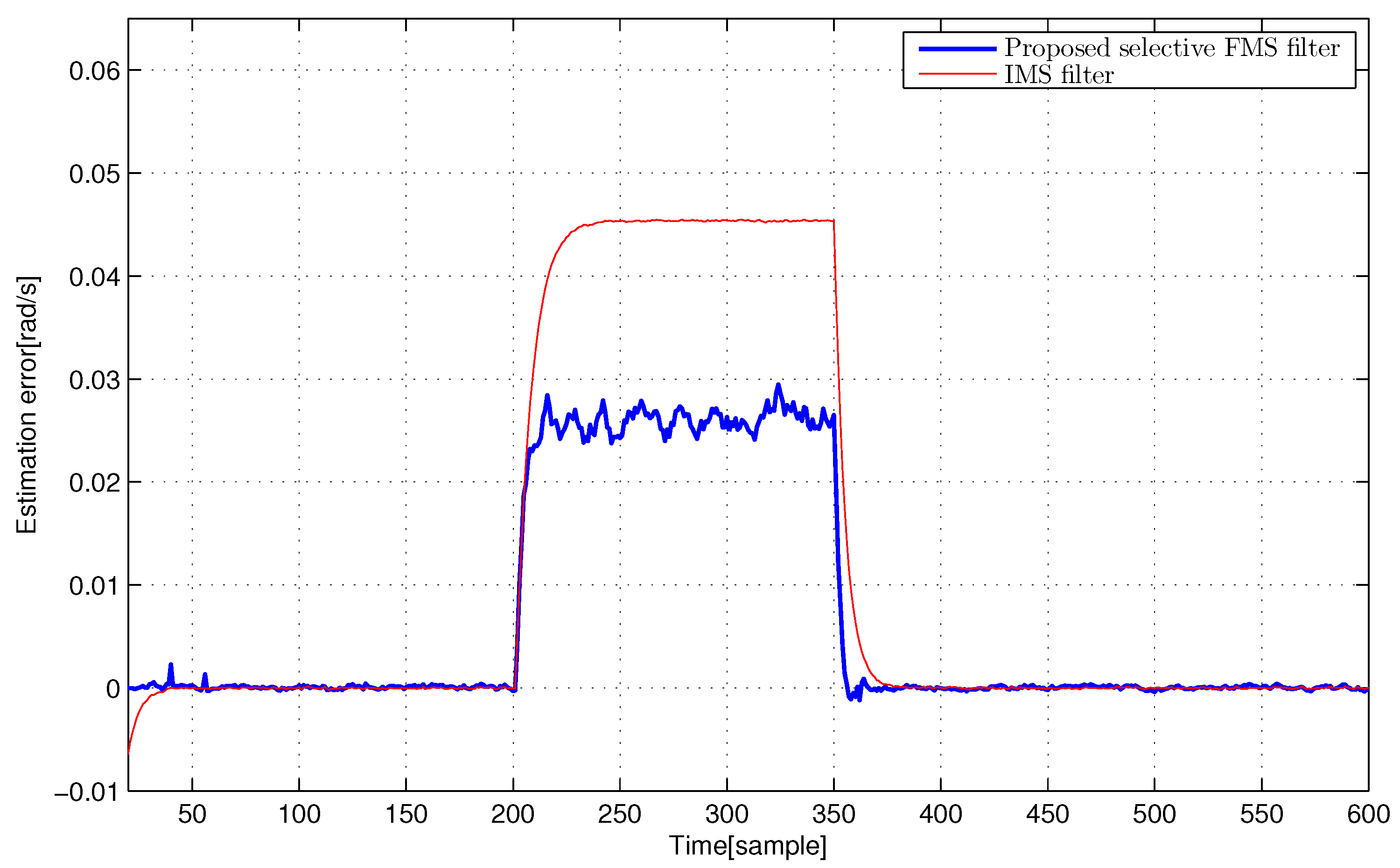
Δ A = δ i 0 0 δ i , Δ C = 0.1 δ i 0 , δ i = 0 . 05 if 200 i 350 , 0 otherwise .
Hence, although two FMS filters x ^ i p (13) and x ^ i s (14) are designed for the nominal state space models (17) and (18) with A and C, they are applied actually for the temporarily uncertain system (19) with model uncertainties (20) and (21), respectively.

4.3. Discussion of Simulation Results

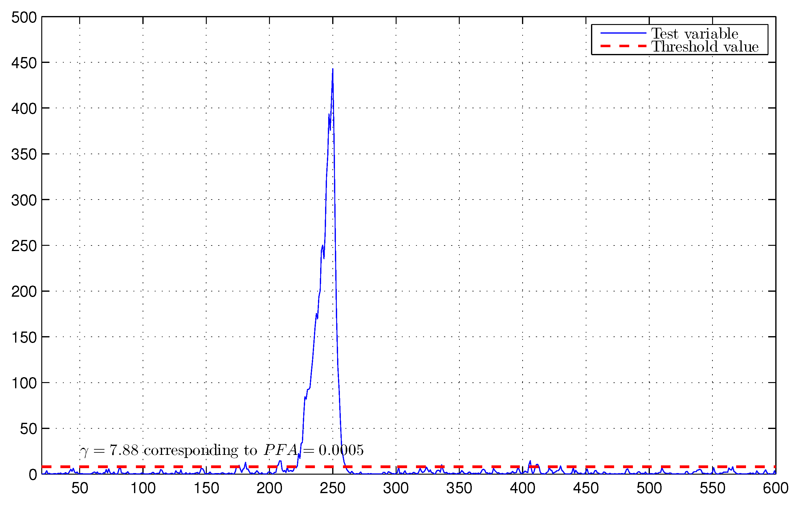
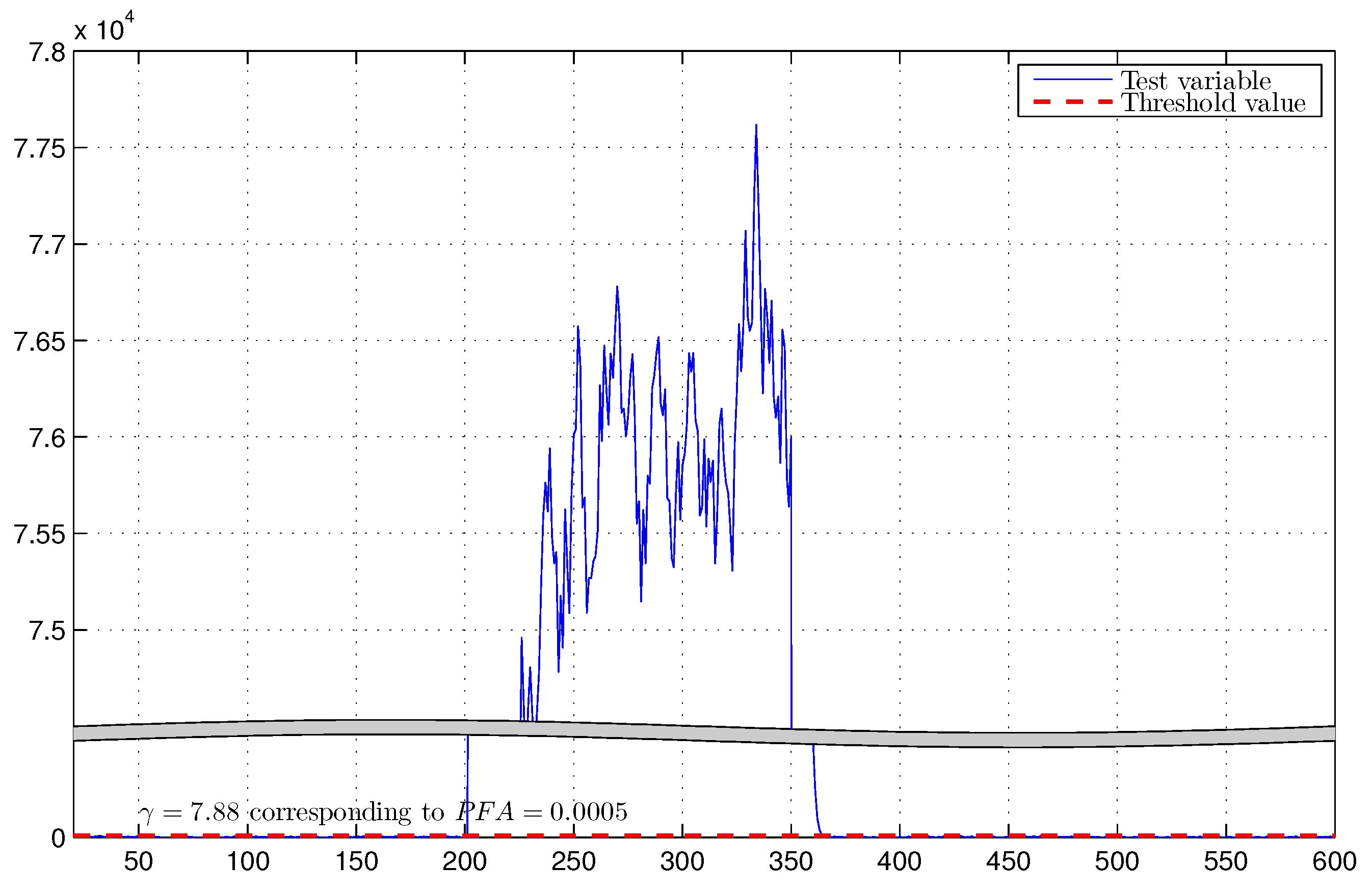
For both systems, the threshold value is set to γ = 7.88 corresponding to PFA=0.0005 in the proposed selective FMS filtering. Figure 2 and Figure 3 show test variables for uncertainty presence and absence declaration.
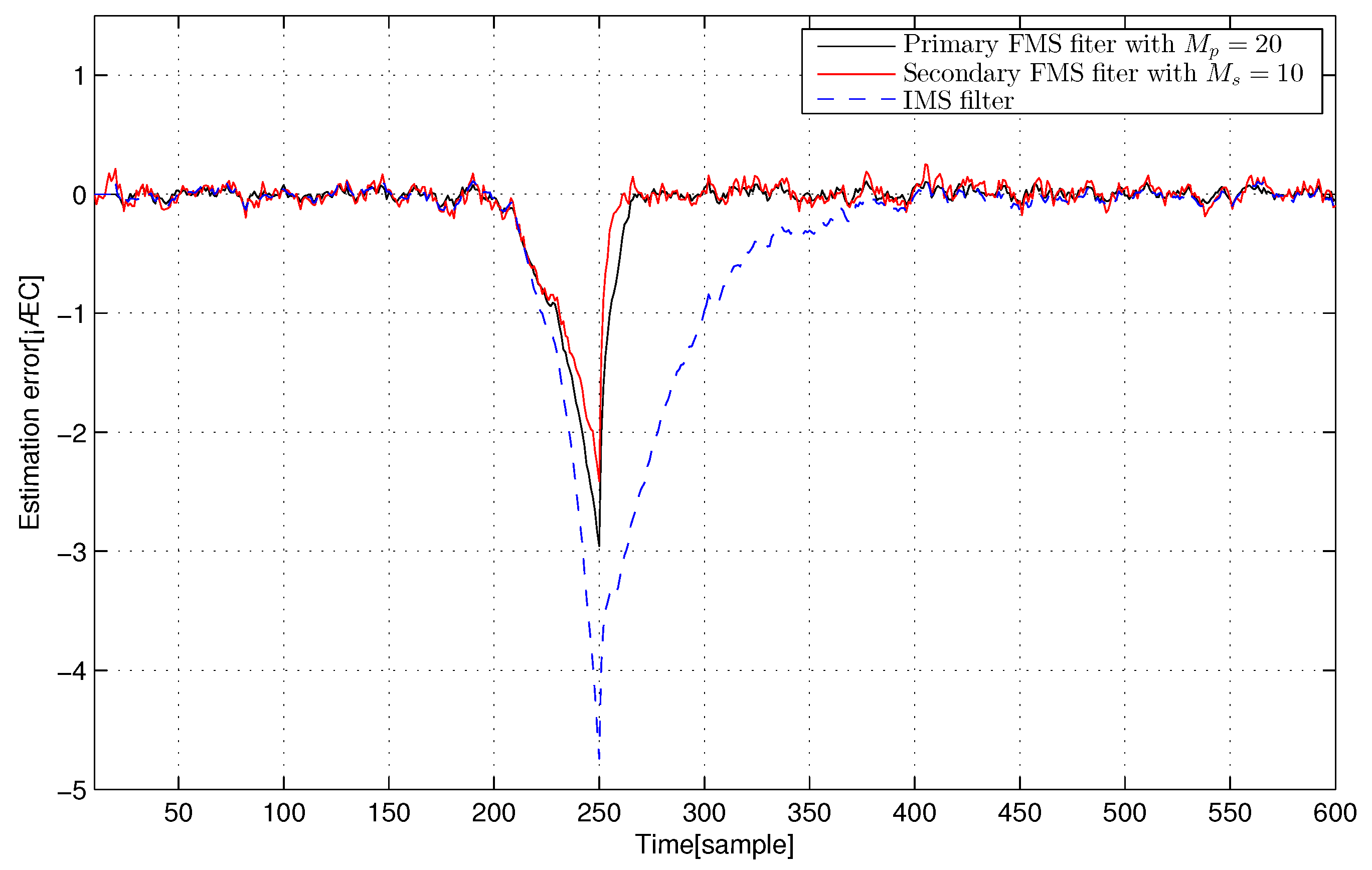
For the F404 gas turbine aircraft engine system, Figure 4 shows estimation errors for the second state indicating turbine temperature for three filters, the primary FMS filter with M p = 20 , the secondary FMS filter with M s = 10 , and the IMS filter. For the electric motor system, Figure 5 shows estimation errors for the second state indicating rotational speed for three filters, the primary FMS filter with M p = 20 , the secondary FMS filter with M s = 10 , and the IMS filter.
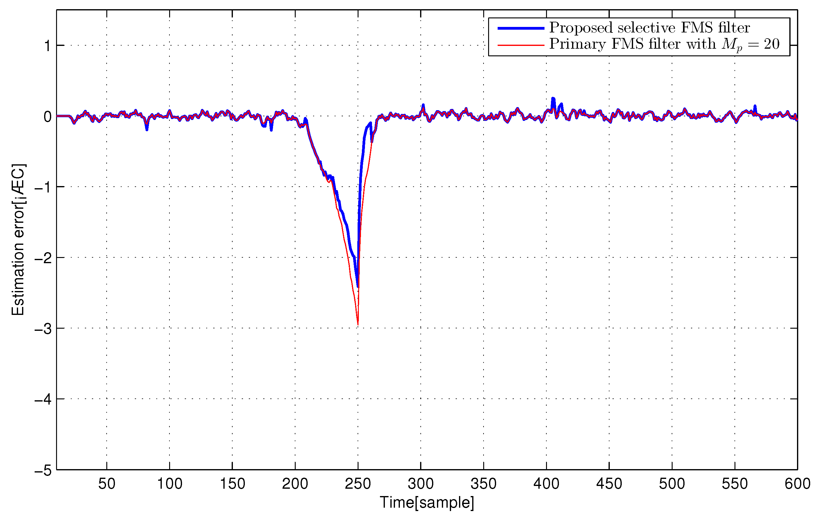
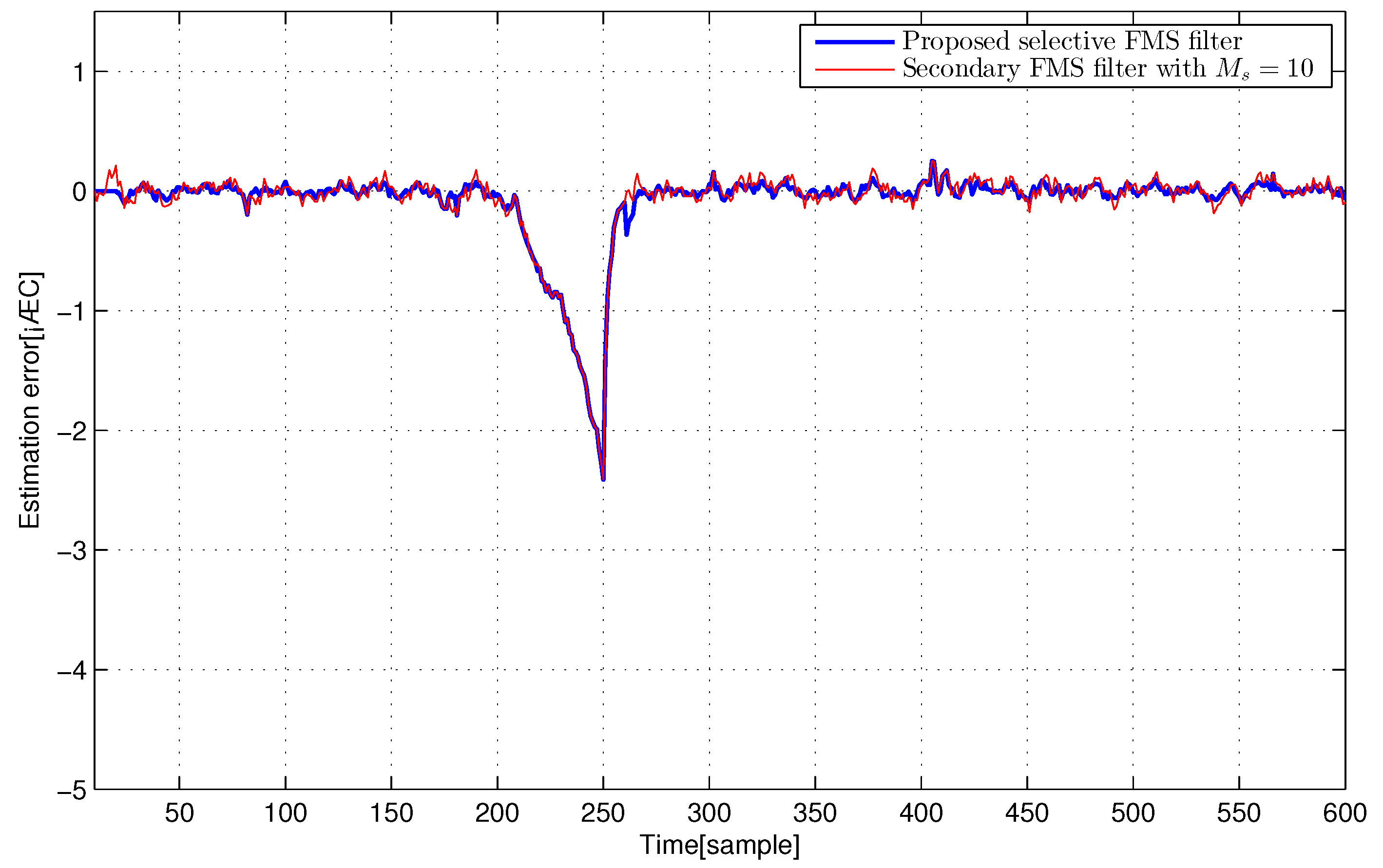
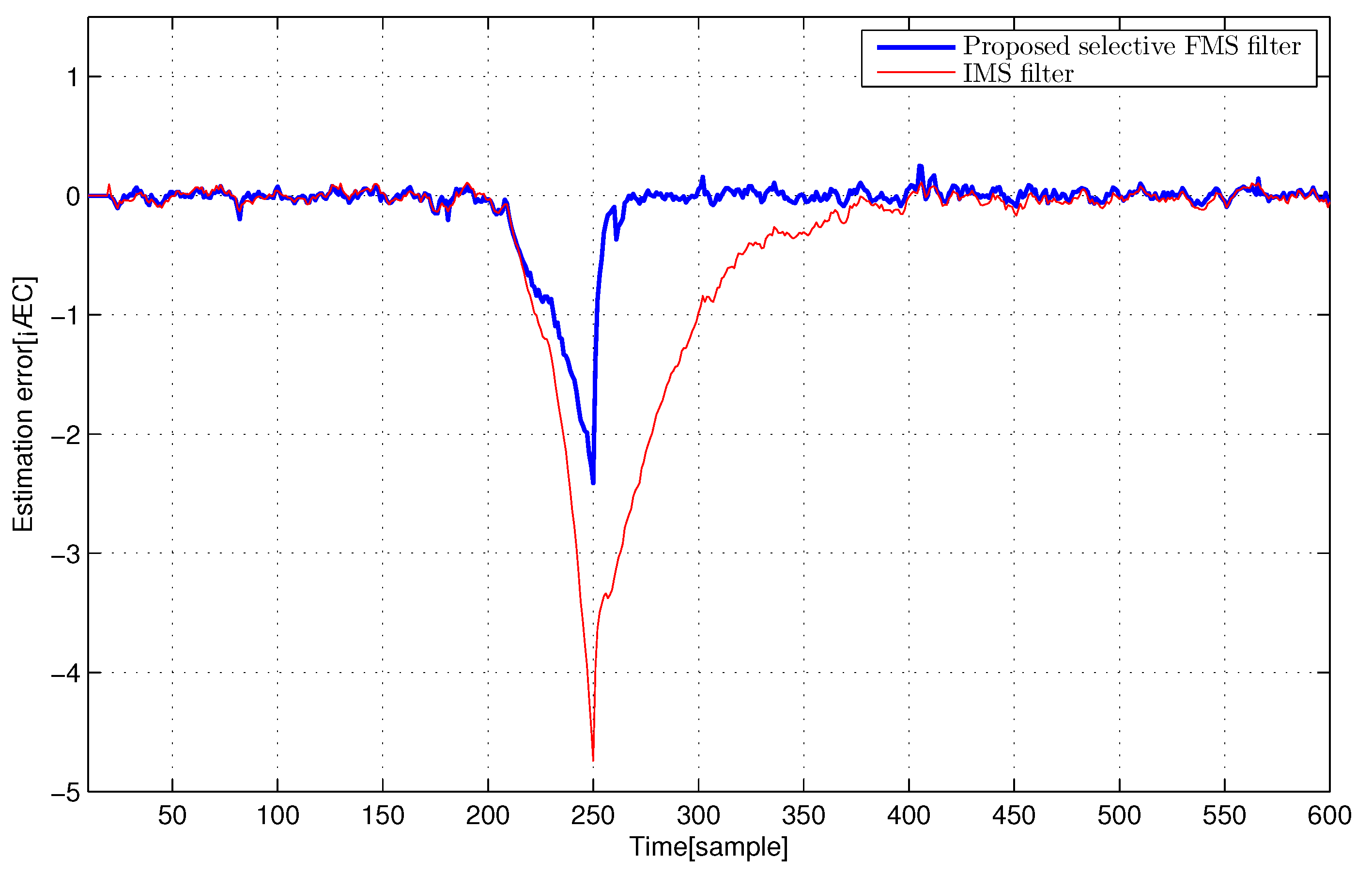
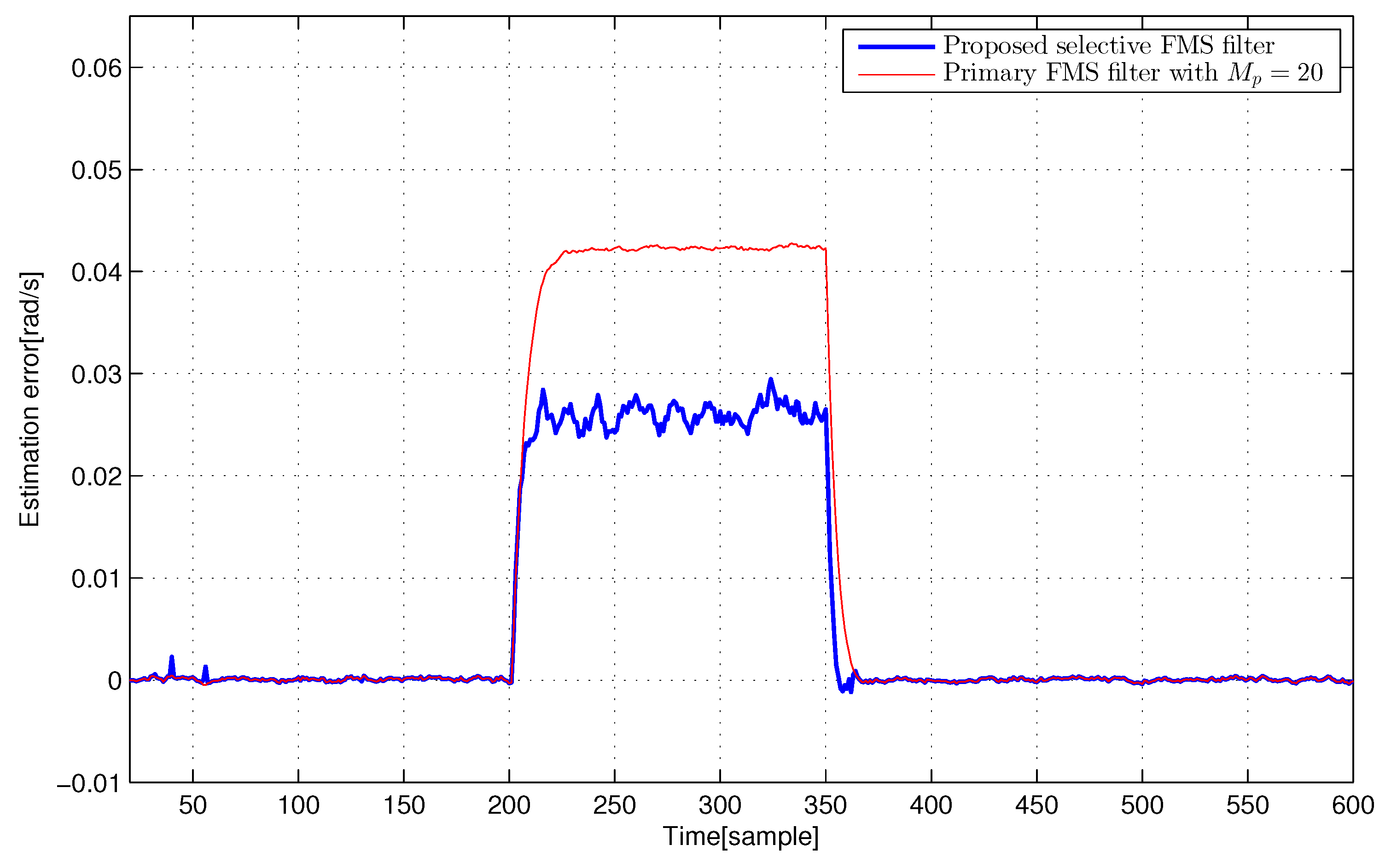
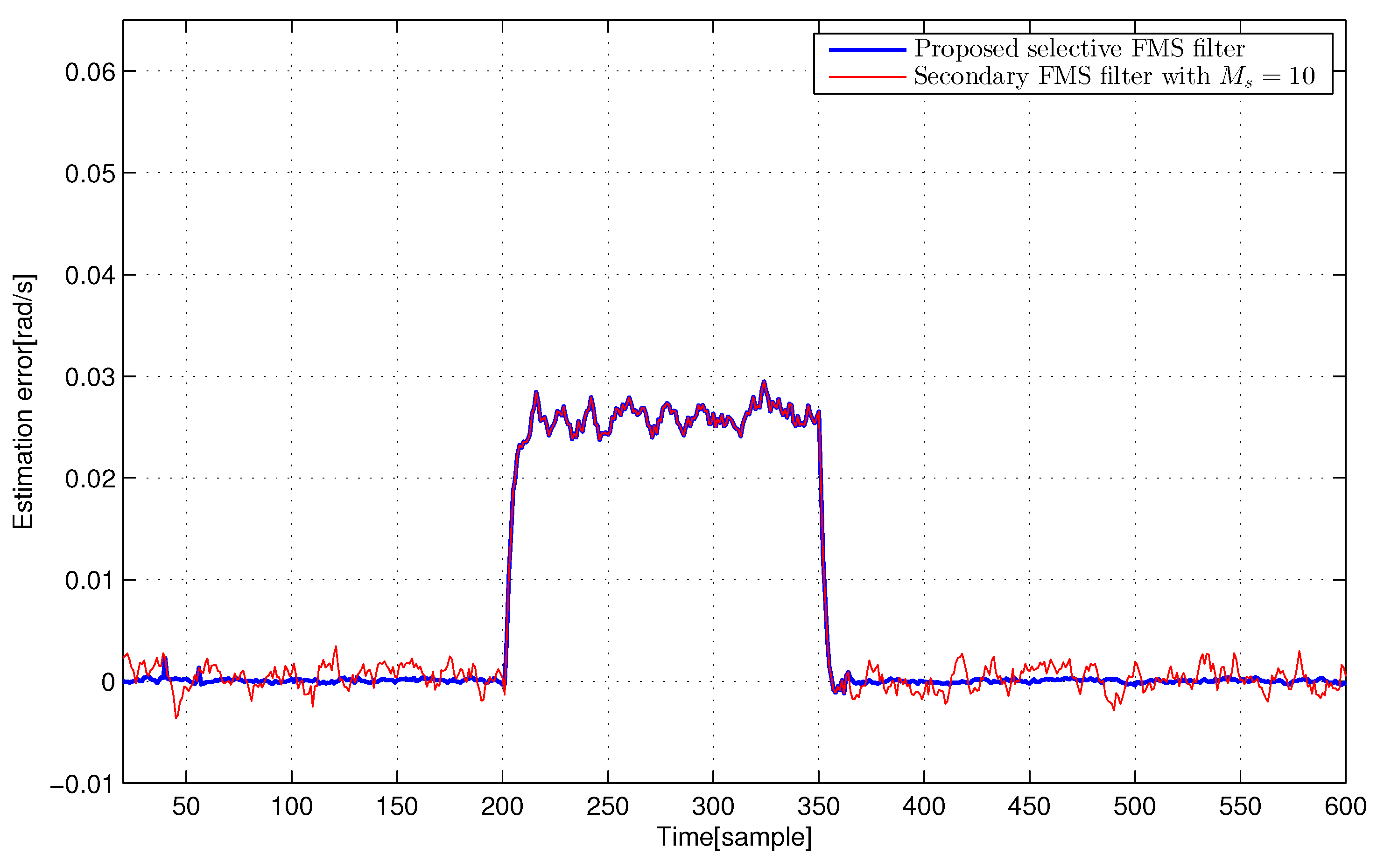
According to the declaration rule (16) using the test variable (15) and the threshold value γ = 7.88 corresponding to PFA = 0.0005, the proposed selective FMS filtering with two kinds of measurement windows provides the state estimate as shown in Figure 6, Figure 7 and Figure 8 and Figure 9, Figure 10 and Figure 11 which show comparisons with three other filters. In addition, time averaged values of root mean square (RMS) estimation errors are presented in Table 1 for 20 simulations. As shown in simulation results, the proposed selective FMS filtering with two kinds of measurement windows can be better than the primary FMS filter and the IMS filter in terms of error magnitude and error convergence on the interval where modeling uncertainty exists. In addition, the proposed selective FMS filtering can be better than the secondary FMS filter when there is no temporary model uncertainty or after temporary model uncertainty is gone. These observations on computer simulations show that the proposed selective FMS filtering can work well in temporarily uncertain systems as well as in certain systems.

5. Conclusions

This paper has proposed selective FMS filtering estimation with two kinds of measurement windows using the chi-square test statistic in order to cover the nominal system as well as the temporarily uncertain system. The simple matrix form for the FMS filter has been developed from the conditional density of the current state given finite past measurements. Then, one of the two FMS filters, the primary FMS filter and the secondary FMS filter, with different measurement windows has been operated selectively to obtain the valid estimate according to the presence or absence of uncertainty. The primary FMS filter has been selected for the nominal system and the secondary FMS filter has been selected for the temporarily uncertain system, respectively. A declaration rule has been defined to indicate the presence or absence of uncertainty, operate the suitable one from two filters, and then obtain the valid filtered estimate. The test variables for the declaration rule have been defined using the chi-squared distribution with one degree of freedom. Finally, extensive computer simulations have been performed for an aircraft engine system as well as an electric motor system to verify the proposed selective FMS filtering with two kinds of measurement windows and compare with existing FMS filtering and IMS filtering. Through simulation results, it has been confirmed that the proposed selective FMS filtering estimation works well for both nominal systems and temporarily uncertain systems. It has been also shown that the proposed selective FMS filter can be remarkably better than the IMS filter for the temporarily uncertain system.
In fact, the research work for the FMS filter is relatively inactive in the case where the system and measurement noises are nonzero-mean Gaussian. Thus, an alternative selective FMS filtering for nonzero-mean noises can be researched as future work.

Funding

This research was funded by National Research Foundation of Korea (NRF-2017R1D1A1B03033024). The APC was funded by Korea Polytechnic University.

Acknowledgments

This research was supported by Basic Science Research Program through the National Research Foundation of Korea funded by the Ministry of Education (NRF-2017R1D1A1B03033024).

Conflicts of Interest

The author declares no conflict of interest.

References

  1. Ardakani, M.; Askarian, M.; Shokry, A.; Escudero, G.; Graells, M.; Espuña, A. Optimal features selection for designing a fault diagnosis system. Comput. Aided Chem. Eng. 2016, 38, 1111–1116. [Google Scholar]
  2. Van, M.; Kang, H.J. Two-stage feature selection for bearing fault diagnosis based on dual-tree complex wavelet transform and empirical mode decomposition. Proc. Inst. Mech. Eng. Part C J. Mech. Eng. Sci. 2016, 230, 291–302. [Google Scholar] [CrossRef]
  3. Hui, K.H.; Ooi, C.S.; Lim, M.H.; Leong, M.S.; Al-Obaidi, S.M. An improved wrapper-based feature selection method for machinery fault diagnosis. PLoS ONE 2017, 12, e0189143. [Google Scholar] [CrossRef] [PubMed]
  4. Vora, S.; Yang, H. A comprehensive study of eleven feature selection algorithms and their impact on text classification. In Proceedings of the 2017 Computing Conference, London, UK, 18–20 July 2017; pp. 440–449. [Google Scholar]
  5. Rajab, K.D. New hybrid features selection method: A case study on websites phishing. Secur. Commun. Netw. 2017, 2017, 9838169. [Google Scholar] [CrossRef]
  6. Cai, J.; Luo, J.; Wang, S.; Yang, S. Feature selection in machine learning: A new perspective. Neurocomputing 2017, 300, 70–79. [Google Scholar] [CrossRef]
  7. Yang, C.; Mohammadi, A.; Chen, Q.W. Multi-sensor fusion with interaction multiple model and chi-square test tolerant filter. Sensors 2016, 16, 1835. [Google Scholar] [CrossRef]
  8. Kang, C.W.; Park, C.G. A soft-failure detection and identification algorithm for the integrated navigation system of lunar lander. Proc. Inst. Mech. Eng. Part G J. Aerosp. Eng. 2016, 230, 2023–2035. [Google Scholar] [CrossRef]
  9. Grewal, M. Applications of Kalman filtering in aerospace 1960 to the present. IEEE Control. Syst. Mag. 2010, 30, 69–78. [Google Scholar] [CrossRef]
  10. Terejanu, G.A. Discrete Kalman Filter Tutorial; University at Buffalo Department of Computer Science and Engineering: Buffalo, NY, USA, 2013. [Google Scholar]
  11. Auger, F.; Hilairet, M.; Guerrero, J.M.; Monmasson, E.; Orlowska-Kowalska, T.; Katsura, S. Industrial applications of the Kalman filter: A review. IEEE Trans. Ind. Electron. 2013, 60, 5458–5471. [Google Scholar] [CrossRef]
  12. Barrau, A.; Bonnabel, S. Invariant Kalman filtering. Annu. Rev. Control. Robot. Auton. Syst. 2018, 1, 237–257. [Google Scholar] [CrossRef]
  13. Shmaliy, Y.S.; Zhao, S.; Ahn, C.K. Unbiased finite impulse response filtering: An iterative alternative to Kalman filtering ignoring noise and initial conditions. IEEE Control. Syst. Mag. 2017, 37, 70–89. [Google Scholar]
  14. Shmaliy, Y.S.; Neuvo, Y.; Khan, S. Review of unbiased FIR filters, smoothers, and predictors for polynomial signals. Front. Signal Process. 2018, 2, 1–29. [Google Scholar]
  15. Zhao, S.; Huang, B.; Shmaliy, Y. Bayesian state estimation on finite horizons: The case of linear statespace model. Automatica 2017, 85, 91–99. [Google Scholar] [CrossRef]
  16. Zhao, S.; Shmaliy, Y.S.; Ahn, C.K.; Luo, L. An improved iterative FIR state estimator and its applications. IEEE Trans. Ind. Inform. 2019, 1–8. [Google Scholar] [CrossRef]
  17. Vazquez-Olguin, M.; Shmaliy, Y.; Ibarra-Manzano, O. Distributed unbiased FIR filtering with average consensus on measurements for WSNs. IEEE Trans. Ind. Inform. 2017, 13, 1140–1147. [Google Scholar] [CrossRef]
  18. Kwon, B.K.; Han, S.; Han, S. Improved receding horizon fourier analysis for quasi-periodic signals. J. Electr. Eng. Technol. 2017, 12, 378–384. [Google Scholar] [CrossRef]
  19. Pak, J.M.; Kim, P.S.; You, S.H.; Lee, S.S.; Song, M.K. Extended least square unbiased FIR filter for target tracking using the constant velocity motion model. Int. J. Control. Autom. Syst. 2017, 15, 947–951. [Google Scholar] [CrossRef]
  20. Kim, P.S. A design of finite memory residual generation filter for sensor fault detection. Meas. Sci. Rev. 2017, 17, 75–81. [Google Scholar] [CrossRef]
  21. You, S.H.; Ahn, C.K.; Shmaliy, Y.S.; Zhao, S. Minimum weighted Frobenius norm discrete-time FIR filter with embedded unbiasedness. IEEE Trans. Circuits Syst. II Express Briefs 2018, 65, 1284–1288. [Google Scholar] [CrossRef]
  22. Xu, Y.; Ahn, C.K.; Shmaliy, Y.S.; Chen, X.; Bu, L. Indoor INS/UWB-based human localization with missing data utilizing predictive UFIR filtering. IEEE/CAA J. Autom. Sin. 2019, 6, 952–960. [Google Scholar] [CrossRef]
  23. Kim, P.S. Finite memory structure filtering and smoothing for target tracking in wireless network environments. Appl. Sci. 2019, 9, 2872. [Google Scholar] [CrossRef]
  24. Matko, V.; Milanović, M. Temperature-compensated capacitance–frequency converter with high resolution. Sens. Actuators A Phys. 2014, 220, 262–269. [Google Scholar] [CrossRef]
  25. Matko, V.; Brezovec, B. Improved data center energy efficiency and availability with multilayer node event processing. Energies 2018, 2018, 2478. [Google Scholar] [CrossRef]
  26. Eustace, R.W.; Woodyatt, B.A.; Merrington, G.L.; Runacres, A. Fault signatures obtained from fault implant tests on an F404 engine. J. Eng. Gas Turbines Power 1994, 116, 178–183. [Google Scholar] [CrossRef]
  27. Messner, B.; Tilbury, D.; Hill, R.; Taylor, J.D. DC Motor Speed: System Modeling: Control Tutorials for MATLAB and Simulink (CTMS); University of Michigan: Ann Arbor, MI, USA, 2017. [Google Scholar]
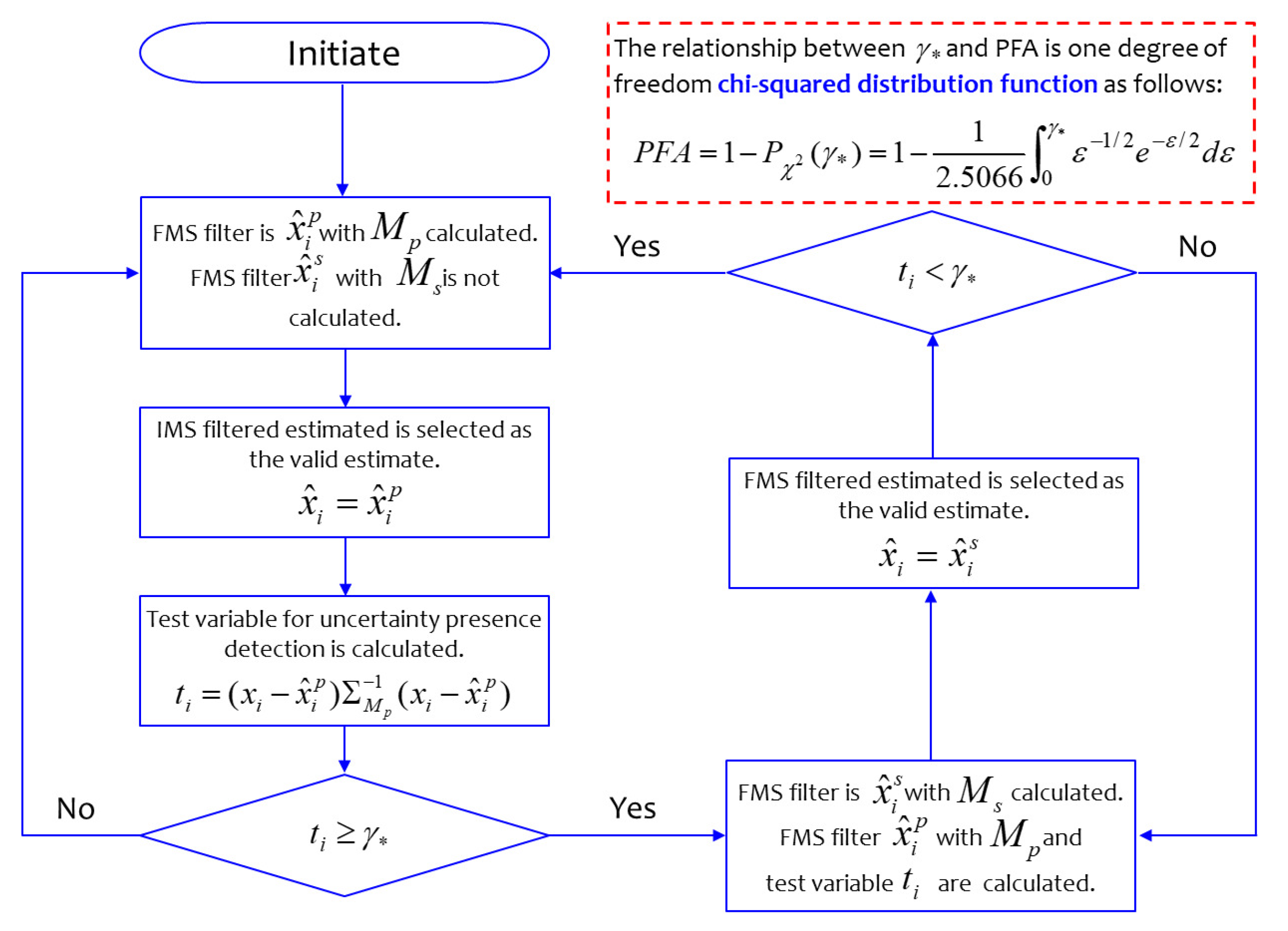
Figure 1. Operation flow for the proposed selective finite memory structure (FMS) filtering. False alarm (PFA).
Applsci 09 04257 g001
Figure 2. Test variable for the F404 gas turbine aircraft engine system.
Applsci 09 04257 g002
Figure 3. Test variable for the electric motor system.
Applsci 09 04257 g003
Figure 4. Estimation errors of primary FMS, secondary FMS and infinite memory structure (IMS) filters for the F404 gas turbine aircraft engine system.
Applsci 09 04257 g004
Figure 5. Estimation errors of the primary FMS, secondary FMS and IMS filters for the electric motor system.
Applsci 09 04257 g005
Figure 6. Estimation errors of the proposed selective FMS and primary FMS filters for the F404 gas turbine aircraft engine system.
Applsci 09 04257 g006
Figure 7. Estimation errors of the proposed selective FMS and secondary FMS filters for the F404 gas turbine aircraft engine system.
Applsci 09 04257 g007
Figure 8. Estimation errors of the proposed selective FMS and IMS filters for the F404 gas turbine aircraft engine system.
Applsci 09 04257 g008
Figure 9. Estimation errors of the proposed selective FMS and primary FMS filters for the electric motor system.
Applsci 09 04257 g009
Figure 10. Estimation errors of the proposed selective FMS and secondary FMS filters for the electric motor system.
Applsci 09 04257 g010
Figure 11. Estimation errors of the proposed selective FMS and IMS filters for the electric motor system.
Applsci 09 04257 g011
Table 1. Comparison of mean of RMS estimation errors.
IMS (Kalman)Primary FMSSecondary FMSSelective FMS
F404 Gas Turbine Aircraft Engine0.08760.03090.03070.0263
Electric Motor0.00250.00230.00160.0015