Article

Space Charge Accumulation and Decay in Dielectric Materials with Dual Discrete Traps

1
State Key Laboratory of Advanced Power Transmission Technology, Global Energy Interconnection Research Institute Co. Ltd., Beijing 102209, China
2
State Key Laboratory of Electrical Insulation and Power Equipment, Xi’an Jiaotong University, Xi’an 710049, China
3
Institute of Fluid Physics, China Academy of Engineering Physics, Mianyang 621900, China
*
Authors to whom correspondence should be addressed.
Appl. Sci. 2019, 9(20), 4253; https://doi.org/10.3390/app9204253
Submission received: 8 September 2019 / Revised: 29 September 2019 / Accepted: 7 October 2019 / Published: 11 October 2019
(This article belongs to the Section Electrical, Electronics and Communications Engineering)

Abstract

:
Charge trapping and de-trapping properties can affect space charge accumulation and electric field distortion behavior in polymers. Dielectric materials may contain different types of traps with different energy distributions, and it is of interest to investigate the charge trapping/de-trapping dynamic processes in dielectric materials containing multiple discrete trap centers. In the present work, we analyze the charge trapping/de-trapping dynamics in materials with two discrete traps in two cases where charges are injected continuously or only for a very short period. The time dependent trapped charge densities are obtained by the integration of parts in the case of continuous charge injection. In the case of instantaneous charge injection, we simplify the charge trapping/de-trapping equations and obtain the analytical solutions of trapped charge densities, quasi-free charge density, and effective carrier mobility. The analytical solutions are in good agreement with the numerical results. Then, the space charge dynamics in dielectric materials with two discrete trapping centers are studied by the bipolar charge transport (BCT) model, consisting of charge injection, charge migration, charge trapping, de-trapping, and recombination processes. The BCT outputs show the time evolution of spatial distributions of space charge densities. Moreover, we also achieve the charge densities at the same position in the sample as a function of time by the BCT model. It is found that the DC poling duration can affect the energy distribution of accumulated space charges. In addition, it is found that the coupling dynamic processes will establish a dynamic equilibrium rather than a thermodynamic equilibrium in the dielectric materials.

Graphical Abstract

1. Introduction

The charge trapping/de-trapping properties determine the formation and accumulation of space charges in dielectric materials [1,2,3,4]. When a dielectric material is subjected to a high electric field, free charges can be injected into the bulk of the material from electrodes [5] or can be generated by ionization [6], and they can be captured by trapping centers, which form space charges. The space charges will accumulate in the bulk when the trapping rate is higher than the de-trapping rate. Such space charges can distort the electric field distribution in the material [7]. Once the local electric field exceeds a threshold value, electric breakdown would occur in the material due to energy released during charge de-trapping [8], multiplication of charge carriers like avalanche [9], or by a strong influence of electromechanical force [10].
Charge trapping/de-trapping dynamics should be influenced by the trap energy of dielectric materials. Trapping centers in polymer dielectric materials can be produced by physical and chemical defects [1]. It is usually assumed that the charges in localized states produced mainly by physical defects (or shallow traps) of polymer dielectric materials are in thermodynamic equilibrium in the time window of experiments such as space charge distribution measurements and transient space charge limited current (SCLC) measurements [1]. In other words, the maximum time constant of charge trapping/de-trapping dynamics in shallow traps is much smaller than the response time of experimental equipment. We can just consider the charge migration in the shallow traps and can neglect their charge trapping/de-trapping dynamics. Nevertheless, chemical impurities can form deep traps in polymers [1]. It will take a very long time for charge trapping/de-trapping dynamics in deep traps to reach an equilibrium state, which is often confirmed by space charge measurements [11,12]. Therefore, the charge trapping/de-trapping dynamics of deep traps should be considered during the analysis of transient electrical properties of dielectric materials, such as transient SCLC, space charge accumulation and dissipation, and transient electroluminescence.
The charge trapping/de-trapping dynamics can be affected by the energy distribution of deep traps in dielectric materials. For single discrete traps, the charge trapping/de-trapping dynamic responses can be obtained analytically by solving the first order charge trapping/de-trapping equation. The space charge responses and external currents or surface potentials have been widely studied theoretically and experimentally in various conditions, such as high electric field [13], electron beam irradiation [14], and corona charging [15]. In the case of multiple discrete traps, Chen et al. developed a charge trapping/de-trapping theory based on two discrete traps [16]. The theory has been used to fit experimental results on space charge build-up and decay in additive-free low-density polyethylene (LDPE) [16,17]. From the fitting of space charge decay curves, the de-trapping probability and trapped charge densities were evaluated. Then, the trap energies and trap densities can be obtained. The trap energies are consistent with those obtained by other experimental techniques such as thermally stimulated current (TSC) [18] and surface potential decay (SPD) [15,19,20], whereas the trap densities are several orders smaller than those calculated by other methods [15,18,21]. One possible reason is that the charge trapping/de-trapping kinetics of two discrete trapping centers cannot be analyzed separately. Moreover, an exponential function was adopted to approximate the energy distribution of traps calculated by the density-functional theory [22]. Then, they assumed that the trap centers are filled with free charges from the bottom to the top. However, the simulation result shows that the trapped charge densities do not increase with time, which is different from the space charge experimental results. This means that the charges in deep traps are not in thermodynamic equilibrium [11,12]. Consequently, we should consider the charge trapping/de-trapping dynamics of deep trapping centers in dielectric materials.
It is of interest to investigate the charge trapping/de-trapping dynamics in polymers with multiple discrete traps. In Section 2, the charge trapping/de-trapping dynamic responses in dielectric materials with multiple discrete traps are investigated analytically. Then, we will study the space charge formation and accumulation properties by a bipolar charge transport (BCT) model. The details of the BCT model are described in Section 3, which consists of processes of injection, migration, trapping, de-trapping and recombination of charges. The simulation results obtained using the BCT model are demonstrated in Section 4. In Section 5, we conclude the main findings of the present work. From dielectric materials with multiple discrete traps, charge transfer between shallow traps and deep traps can influence the space charge accumulation and dissipation properties. Charging the dielectric materials for a longer time, more charges could be captured by deep traps so that the space charges decay much slower. The charges trapped in deep trapped can distort the local electric field and may result in ageing of the dielectric materials.

2. Dynamic Responses of Charge Trapping and De-trapping

2.1. Charge Trapping/De-trapping Dynamics

Free charges in extended states or quasi-free charges in localized states produced by injection, irradiation, or ionization can be captured by traps in dielectric materials with a trapping probability. The charge trapping properties were investigated theoretically and experimentally by considering the relationship between the Langevin recombination model and the Shockley-Read-Hall (SRH) recombination model. It was found that the probability of trapping of charge carriers PT in deep trap centers is proportional to the mobility carriers µ0 and the trap density of the material NT, and is inversely proportional to the permittivity [23,24]. Namely, PT can be given by,
P T = μ 0 e N T / ε 0 ε r
where µ0 is the shallow-trap-controlled carrier mobility in m2 V−1 s−1, e is the elementary charge in C, ε0 is the permittivity of vacuum in Fm−1, and εr is the relative permittivity of dielectric materials. For LDPE, εr equals to 2.3.
The charge trapping probability given by Equation (1) is proportional to the carrier mobility, which is consistent with the comments of Toomer et al. [15]. It was pointed out that the charge trapping probability would be related to the thermal velocity of carriers in the case of extended state conduction, nevertheless, this would depend on the drift velocity in the case of charge hopping in localized states. When the shallow-trap-controlled carrier mobility is set as 10−13–10−14 m2 V−1 s−1, the charge trapping probability estimated by Equation (1) will be 4.91 × 10⁻¹–4.91 × 10⁻² s−1, which are in good agreement with the previous findings [15,25,26,27].
The trapped charges can be released to the transport states after having been trapped in trap centers for a period. The thermally-assisted de-trapping probability is given as [26],
P D ( E T ) = υ ATE exp ( E T / k B T )
where υATE = kBT/hp, is the attempt-to-escape frequency in s−1 [22,28]. Here, hp is the Planck constant in Js.
The charge trapping and de-trapping dynamics in insulators with multiple trap levels can be described by the first-order charge trapping and de-trapping dynamic equation. It is assumed that charge trapping events into various trap levels are incompatible and charge de-trapping events from various traps are mutually independent, as shown in Figure 1. In the present work, we just consider the charge trapping/de-trapping dynamics at two discrete trap levels, namely, trap level 1 and trap level 2. The energies and densities of deep trap level 1 and deep trap level 2 are ET1 and ET2, QT1 and QT2, respectively.
d q free d t = q free i = 1 n P Ti ( 1 q trapi Q Ti ) + i = 1 n P Di q trapi
d q t r a p i d t = q f r e e P T i ( 1 q t r a p i Q T i ) P D i q t r a p i , i = 1 , 2 , , n
where qfree and qtrap are the densities of free and trapped charges in Cm−3, while QT equals to eNT and n is the number of deep trap levels, where n = 2 in the present work; furthermore, t is the time.
We will analyze the charge trapping and de-trapping dynamic responses in the following two cases. Namely, in the first case, free charges are assumed to be injected continuously to compensate for the depletion of free charges in the bulk caused by trapping. In other words, the free charges are injected to keep the total number of free charges in the bulk at a constant value. In contrast, a certain number of free charges are injected instantaneously only for a short period in the second case. In present work, T is set as 300 K. The assigned values of carrier mobility, trap energies, and trap densities are listed in Table 1 [17].

2.2. Continuous Charge Injection

First, we consider the first case where the free charges are injected continuously. As mentioned above, we assumed that the free charges injected continuously to keep the total number of free charges in the bulk unchanged. In this condition, we can derive the following first-order charge trapping/de-trapping equation to obtain the time-dependent trapped charge density, qtrapi(t).
d q t r a p i ( t ) d t = q f r e e 0 P T i ( 1 q t r a p i Q T i ) P D i q t r a p i , ( i = 1 , 2 )
Equation (5) can be rearranged by moving dt to the right and the term including qtrapi to the left part of the equation. Integrating the left and right parts of the rearranged equation, we can obtain the following equation,
( q f r e e 0 P T i Q T i + P D i ) q t r a p i ( t ) q f r e e 0 P T i = C exp [ ( q f r e e 0 P T i Q T i + P D i ) t ] , ( i = 1 , 2 )
where C is an undetermined coefficient.
It is assumed that there are no charges in the traps at the beginning of the charge trapping/de-trapping process. The undetermined coefficient C in Equation (6) can be estimated by this initial condition qtrapi(0) = 0. Consequently, the trapped charge density as a function of time qtrapi(t) can be derived as,
q t r a p i ( t ) = q f r e e 0 P T i Q T i q f r e e 0 P T i + P D i Q T i × [ 1 exp [ ( q f r e e 0 P T i Q T i + P T i ) t ] ] , ( i = 1 , 2 )
Equation (6) shows that the trapped charge density, qtrapi(t), increases monotonically with an increase in time until it approaches its maximum value, which is equal to qfree0PTiQTi/(qfree0PTi+PDiQTi). The largest increasing rate of qtrapi(t) is qfree0PTi that appears at t = 0. Then, the increasing rate decreases gradually with time.

2.3. Instantaneous Charge Injection

When a certain fixed number of free charges qtotal is assumed instantaneously, it is difficult to obtain the analytical solutions for the charge trapping/de-trapping Equations (3) and (4). Nevertheless, when trapped charge densities, qtrapi(t), are always much smaller than the densities of trap centers in a dielectric material, qtrapi(t)/QTi can be approximated by zero, and the ordinary differential equations can be solved analytically. The first order charge trapping/de-trapping equations in the dielectric materials containing two discrete trap levels can be simplified as the following equations.
d q t r a p 1 d t = ( P T 1 + P D 1 ) q t r a p 1 P T 1 q t r a p 2 + P T 1 q t o t a l
d q t r a p 2 d t = P T 2 q t r a p 1 ( P T 2 + P D 2 ) q t r a p 2 + P T 2 q t o t a l
Given PTi, PDi, and qtotal, Equations (8) and (9) are linear system of differential equations with constant coefficients. The undetermined function qtrap2(t) and the first-order derivative dqtrap2(t)/dt can be expressed as functions of qtrap1(t), dqtrap1(t)/dt, and d2qtrap1(t)/dt2 by Equation (8). We can eliminate qtrap2(t) and dqtrap2(t)/dt in Equation (9) to obtain the linear differential equation of second order with constant coefficients of qtrap1(t). Similarly, we can find the second order linear differential equation with constant coefficients of qtrap2(t).
d 2 q t r a p 1 d t 2 + ( P T 1 + P D 1 + P T 2 + P D 2 ) d q t r a p 1 d t + ( P T 1 P D 2 + P T 2 P D 1 + P D 1 P D 2 ) q t r a p 1 P T 1 P D 2 q t o t a l = 0
d 2 q t r a p 2 d t 2 + ( P T 1 + P D 1 + P T 2 + P D 2 ) d q t r a p 2 d t + ( P T 1 P D 2 + P T 2 P D 1 + P D 1 P D 2 ) q t r a p 2 P T 2 P D 1 q t o t a l = 0
The second order linear differential Equations (10) and (11) have the same characteristic equation.
r 2 + ( P T 1 + P D 1 + P T 2 + P D 2 ) r + P T 1 P D 2 + P T 2 P D 1 + P D 1 P D 2 = 0
Solving the characteristic Equation (12), we can obtain two unequal real roots, namely λ1 and λ2. Then, we can solve the second order linear inhomogeneous differential Equations (10) and (11). The time dependent trapped charge densities qtrap1(t) and qtrap2(t) are given by,
q t r a p 1 ( t ) = C 11 exp ( λ 1 t ) + C 12 exp ( λ 2 t ) + P T 1 P D 2 q t o t a l / ( P T 1 P D 2 + P T 2 P D 1 + P D 1 P D 2 )
q t r a p 2 ( t ) = C 21 exp ( λ 1 t ) + C 22 exp ( λ 2 t ) + P T 2 P D 1 q t o t a l / ( P T 1 P D 2 + P T 2 P D 1 + P D 1 P D 2 )
where C11, C12, C21, and C22 are coefficients dependent on the initial conditions. The analytical solutions of coefficients C11, C12, C21, and C22 are shown in Appendix A.
Substituting Equations (13) and (14) into qfree(t) = qtotalqtrap1(t) − qtrap2(t), we can calculate the time dependent free charge density.
q f r e e ( t ) = P D 1 P D 2 q t o t a l / ( P T 1 P D 2 + P T 2 P D 1 + P D 1 P D 2 ) ( C 11 + C 21 ) exp ( λ 1 t ) ( C 12 + C 22 ) exp ( λ 2 t )
In the case of constant total charge density, the time dependent effective carrier mobility, μeff(t), has a similar function as qfree(t).
μ e f f ( t ) = μ 0 P D 1 P D 2 / ( P T 1 P D 2 + P T 2 P D 1 + P D 1 P D 2 ) μ 0 [ ( C 11 + C 21 ) e x p ( λ 1 t ) ( C 12 + C 22 ) exp ( λ 2 t ) ] / q t o t a l
When the approximation, qtrapi(t)/QTi ≈ 0, is not valid for i = 1 or 2, alternatively, we can solve the charge trapping/de-trapping equations numerically by an unconditionally stable nonstandard finite differential (NSFD) method [29]. First, the charge trapping term and the charge de-trapping term in the charge trapping/de-trapping Equation (3) is split into two parts. Secondly, we just solve the charge trapping term in the differential equation of free charge density, and the de-trapping terms in the differential equations of trapped charge densities by the NSFD method.
d q f r e e ( t ) d t = q f r e e ( t ) i = 1 n P T i ( 1 q t r a p i ( t ) Q T i )
d q t r a p i ( t ) d t = P D i q t r a p i ( t ) , ( i = 1 , 2 )
It is assumed that ∆t is the time step size, and [tk = kt]k≥0 is a sequence of equally-spaced time points. Then, the differential equations can be transformed into difference equations. Adopting the NSFD scheme, we can obtain the numerical form of Equations (17) and (18) as follows:
q f r e e ( t k + 1 ) = q f r e e ( t k ) exp [ i = 1 n P T i ( 1 q t r a p i ( t k ) / Q T i ) Δ t ]
q t r a p i ( t k + 1 ) = q t r a p i ( t k ) exp ( P D i Δ t ) ,   i = 1 , 2
The numerical forms are unconditionally stable regardless of ∆t, which is superior to the finite different method (FDM). According to Chapwanya et al. [29], the Lambert W function is used in Equations (19) and (20) (the NSFD scheme) to increase the accuracy of numerical solutions. Thirdly, the charge de-trapping term in the differential equation of free charge density and the charge trapping terms in the differential equation of trapped charge densities can be computed explicitly using the trapped charge densities and free charge densities at tk+1 obtained by the NSFD scheme. Then, we can obtain numerical solutions of free charge density qfree(tk+1) and trapped charge densities qtrapi(tk+1) at tk+1.
Figure 2a,b shows the analytical and numerical results of free charge density and trapped charge densities as a function of time with the total charge densities of 2 cm−3 and 10 cm−3, respectively. When the total charge density is relatively low (e.g., 2 cm−3), the approximations, qtrapi(t)/QTi ≈ 0, are valid, and the analytical results are in good agreement with the numerical results. Nevertheless, when the total charge density is relatively high (e.g., 10 cm−3), the approximations, qtrapi(t)/QTi ≈ 0, are not always valid. Therefore, a small difference occurs between the analytical results and the numerical results in the time range from 103 to 104 s. However, the shape of the curves is nearly the same.
The free charge density decays exponentially with time both in Figure 2a,b. The trapped charge density in trap level 2, qtrap2(t), increases with time during the charge trapping/de-trapping process. Whereas, the trapped charge density in trap level 1, qtrap1(t), increases firstly and then decreases with time. Since the trapping probability of trap center is proportional to the trap density, the trapping probability of trap level 1 will be five times larger than that of trap level 2. Consequently, more free charges are captured by trap level 1 at the beginning. In addition, the time needed to reach steady state for charges in trap level 2 is prolonged in the presence of trap level 1.

2.4. Steady State Characteristics in the Case of Instantaneous Charge Injection

When the charge trapping/de-trapping dynamics reach steady-state tst, namely dqtrapi(t)/dt = 0, the exact relationship between trapped charge densities and free charge density can be obtained from the charge trapping/de-trapping differential equations.
q t r a p i ( t s t ) = P T i q f r e e ( t s t ) q e N T i P T i q f r e e ( t s t ) + P D i q e N T i
Using the above equation, we can calculate trapped charge densities in each trap center as a function of free charge density at steady state, as shown in Figure 3a. For small free charge densities, the relations between the trapped charge densities and the free charge densities are linear, qtrapi(tst)∝qfree(tst). For high free charge densities, the traps will be fully filled. Moreover, the deeper traps will be fully filled first, then the shallower traps.
The quantitative relationship among qfree(tst), qtrap1(tst), and qtrap2(tst) can be derived from Equations (13)–(15) for small free charge densities. The relationship is,
q f r e e ( t s t ) / q t r a p 1 ( t s t ) / q t r a p 2 ( t s t ) = P D 1 P D 2 / P T 1 P D 2 / P T 2 P D 1
Substituting the charge trapping probability and charge de-trapping probability equations into Equation (22), we can obtain the relationships between qfree(tst) and qtrapi(tst), and between qtrap1(tst) and qtrap2(tst).
q f r e e ( t s t ) q t r a p i ( t s t ) = ε 0 ε r υ A T E q e N T i μ 0 exp ( E T i k B T )
q t r a p 1 ( t s t ) q t r a p 2 ( t s t ) = N T 1 N T 2 exp ( E T 2 E T 1 k B T )
Equations (23) and (24) show that the trapped charge densities increase exponentially with the increasing trap energy at a given qfree(tst). Accordingly, at steady state deeper traps will be fully filled first, as demonstrated in Figure 3b. However, ratios of qtrap1(tst) to qtrap2(tst) at transient sates are different from the results of Equation (24). As indicated in Figure 2, qtrap1(tst) could be much larger than qtrap2(tst) at transient states. The exact relationship between qtrap1(tst) and qtrap2(tst) is demonstrated in Appendix B.
Figure 3b demonstrates the dependences of total charge density, qtotal(tst), and effective carrier mobility, μeff(tst), on free charge density. The total charge density increases with increasing free charge density. The two convex inflection points in qtotal(tst)–qfree(tst) curve imply the fully filling of trap level 1 and trap level 2. The effective carrier mobility is a constant for small free charge densities. Then, the effective carrier mobility rises as the free charge density increases.

3. Bipolar Charge Transport Model

In dielectric materials subjected to voltages, the injected charges will not only be captured by trapping centers, but also migrate in the shallow traps [1]. We will utilize the bipolar charge transport (BCT) model to investigate the space charge dynamics in the dielectric materials with two discrete traps. We consider a system consisting of a dielectric material with the thickness of L clamped by two electrodes. A one-dimensional coordinate, x, is set up for the sample. X = 0 corresponds to the interface between the material and cathode, and x = L corresponds to the interface between the material and anode. The schematic of the BCT model of dielectric materials subjected to electric fields is shown in Figure 4.

3.1. Charge Injection

We can use Schottky thermionic emission with an effective injection barrier to model the charge injection process from the electrode to the insulation material. Since concentrating on the space charge evolution and charge trapping/de-trapping dynamics in the bulk of the material containing two discrete trap levels in the present work, we describe the charge injection processes for electrons and holes by Schottky thermionic emission with effective injection barriers [22,30].
j i n e ( 0 , t ) = A T 2 exp ( E i n e k B T ) exp ( E S c h ( 0 , t ) k B T 1 )
j i n e ( L , t ) = A T 2 exp ( E i n h k B T ) exp ( E S c h ( 0 , t ) k B T 1 )
where jine(0,t) and jinh(L,t) are the thermionic injection currents at cathode-insulator interface and anode-insulator interface in Am−2, respectively. A is the Richardson constant; Eine and Einh are the contact potential barrier at the cathode-insulator interface and anode-insulator interface in eV, respectively. ESch is the Schottky potential barrier lower, Esch = (qeF/4πε0εr)1/2. F is the electric field in the dielectric material in Vm−1.

3.2. Self-Consitent Equations

The charges in dielectric materials are governed by a set of self-consistent equations [22,30,31].
(a) Charge advection-reaction equations,
q f r e e ( x , t ) t + j c ( x , t ) x = S f r e e ( x , t )
q t r a p i ( x , t ) t = S t r a p i ( x , t ) , ( i = 1 , 2 )
(b) Charge transport equation,
j c ( x , t ) = q f r e e ( x , t ) μ 0 F ( x , t )
(c) Poisson’s equation,
2 ϕ ( x , t ) x 2 = q f r e e ( x , t ) + i = 1 2 q t r a p i ( x , t ) ε 0 ε r
(d) The spatial integration of electric field,
V a p p l = 0 L F ( x , t ) d x
where qfree and qtrap are the free and trapped charge densities in the dielectric in cm−3, respectively; jc is the conducting current density in the material in Am−2; D it the diffusion coefficient of free charges which is equal to μ0kBT/qe; ϕ is the potential in the material in V; and Vappl is the applied voltage on the sample in V. The summation of free and trapped charge densities is named as net charge density, qnet.

3.3. Charge Reaction Dynamics

The following four equations represent the first order charge dynamics in dielectric materials having two discrete trap levels, including charge trapping/de-trapping and recombination processes [22,30].
S e μ = R e μ , h μ q f r e e ( e ) q f r e e ( h ) i = 1 n R e μ , h t q f r e e ( e ) q t r a p ( h ) i q f r e e ( e ) i = 1 n P T ( e ) i ( 1 q t r a p ( e ) i / q e N T ( e ) i ) + i = 1 n P D ( e ) i q t r a p ( e ) i
S e t i = q f r e e ( e ) P T ( e ) i ( 1 q t r a p ( e ) i / q e N T ( e ) i ) P D ( e ) i q t r a p ( e ) i R e t , h μ q t r a p ( e ) i q f r e e ( h ) , i = 1 , 2
S e μ = R e μ , h μ q f r e e ( e ) q f r e e ( h ) i = 1 n R e t , h μ q t r a p ( e ) i q f r e e ( h ) q f r e e ( h ) i = 1 n P T ( h ) i ( 1 q t r a p ( h ) i / q e N T ( h ) i ) + i = 1 n P D ( h ) i q t r a p ( h ) i
S e t i = q f r e e ( h ) P T ( h ) i ( 1 q t r a p ( h ) i / q e N T ( h ) i ) P D ( h ) i q t r a p ( h ) i R e μ , h t q f r e e ( e ) i q t r a p ( h ) , i = 1 , 2
where S, Set, Shμ, and Sht are the charge sources of mobile and trapped electrons and holes, respectively; and n = 2. Reμ, hμ is the recombination rate between free electrons and free holes in cm−3 s−1. Reμ,ht and Ret,hμ are the recombination rate between free electrons and trapped holes and the recombination rate between trapped electrons and free holes in Cm−3s−1, respectively.
In the Langevin recombination model, the recombination rate between free electrons and free holes is determined by the carrier motilities of electrons and holes [30,32], Reμ,hμ = (μe0 + μh0)/ε0εr. The recombination rate between free electrons and trapped holes is determined by the carrier motility of free electrons; and the recombination rate between trapped electrons and free holes is determined by the carrier motility of free holes [30,32], namely, Reμ,ht = μe0/ε0εr and Ret,hμ = μh0/ε0εr.

3.4. Numerical Techniques

The charge advection-reaction equation is split into two parts, namely, the charge advection equation and the charge reaction equation, by the Strang splitting method. The charge reaction equations for free charges and trapped charges are resolved by the NSFD scheme [29]. The charge advection equation is solved by the weighted essentially non-oscillatory method (WENO), which can provide highly stable and accurate numerical charge distribution results [33].
Poisson’s equation is solved by the Boundary Element Method (BEM) with Dirichlet boundary condition [34]. The BEM method is discretized spatially in integral forms by utilizing functional analysis. The advantages of BEM method are that they can simultaneously calculate the potentials and electric fields in the dielectric material and can obtain the electric field at every point of the discretization grid, particularly on the interfaces between electrodes and dielectric material.

4. Results and Discussion

An additive-free LDPE film with a thickness of 150 μm was used in the BCT simulations. The film was discretized into 300 elements, respectively. The computation time interval Δt was set as 0.01 s, which satisfied the Courant-Friedrich-Levy (CFL) law [35]. The charge injection barriers for electrons and holes are set as 1.1 eV and 1.3 eV, respectively. Symmetrical values for parameters of carrier mobilities, densities and energies of trap levels 1 and 2 are used in the BCT simulations, which are given in Table 1. It is assumed there are no charges inside the dielectric material at initial states. Charges are injected into the material via Schottky thermionic emissions and flow out the material with Ohm’s law.

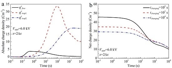
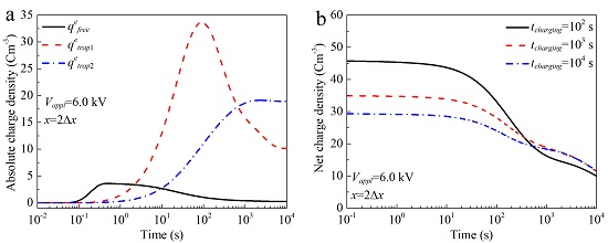
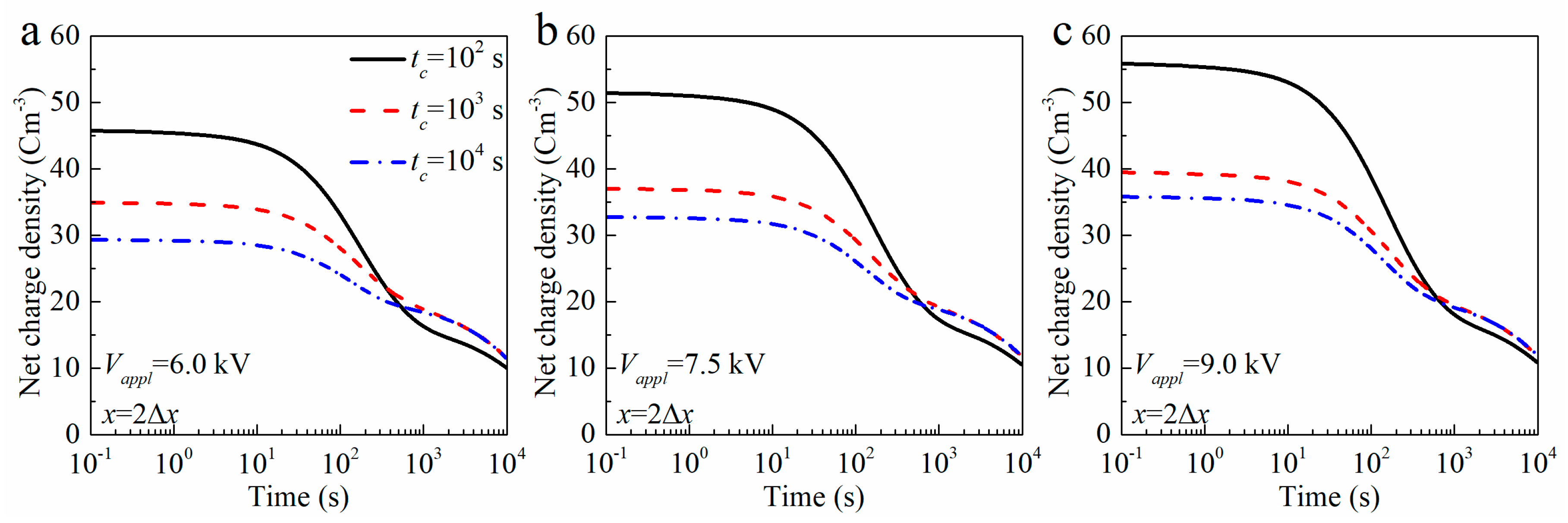
4.1. Space Charge Accumulation Characteristics

Free charge and trapped charge densities are dependent on time and position. The BCT model outputs of free charge density and net charge density distributions in the material at various times show that the accumulated negative charges are much larger than the accumulated positive charges in the bulk of LDPE. Since the contact potential barrier between the cathode and the dielectric material is lower than that between the anode and the material, the emission rate of electrons is much higher than the emission rate of holes according to the Schottky thermionic emission equation. For example, the injection current densities of electrons and holes are about 7.36 × 10⁻³ Am−2 and 3.21 × 10⁻⁶ Am−2, respectively, at the voltage of 6.0 kV at the beginning of voltage application. Accordingly, the injected negative charges are much larger than the injected positive charges.
When the space charges are only caused by charge injections from contact electrodes, homogenous space charges will be accumulated in the dielectric material. The injected electrons drift in the bulk of the material towards the anode and are captured by trapping level 1 and trapping level 2 gradually. If the trapping rates are larger than the de-trapping rates, most of the injected electrons are trapped in the trapping centers. The trapped electrons can distort the electric fields in the vicinity of the cathode, reducing the Schottky thermionic emission current. This will lead to the saturation of accumulated space charges in the dielectric material.
Figure 5a indicates the average net charge density as a function of time in the dielectric material subjected to various voltages. The average net charge density equals to the integration of net charge density over position x divided by the length of the dielectric material. The average net charge densities increase very fast at the beginning of the application of voltage. Then, the increasing rates of the average net charge densities decline gradually with time. In addition, the time needed for the space charge accumulation to reach steady-state decreases with increasing the applied voltage. Figure 5b shows the external current densities as a function of elapsed time after the application of voltages. Since no free charges are assumed inside the dielectric material before the application of voltage, the current density is very small at the beginning after applying voltage to the sample due to low density of free charges. With increasing the elapsed time of voltage application, more and more charges are injected into the dielectric material, so the current density increases with time until the front of injected charges reaches the opposite electrode. The peaks correspond to the transit time of free charges, which is 4.8 s at 6.0 kV, 4 s at 7.5 kV, and 3.4 s at 9.0 kV. After the injected charges reach the opposite electrode charge trapping process will dominate the charge transport in the dielectric material and the current density decrease monotonically with time. Stepwise reductions can be observed in the time-dependent current density, which are caused by charge trapping-de-trapping dynamics between the extended states and two deep traps.

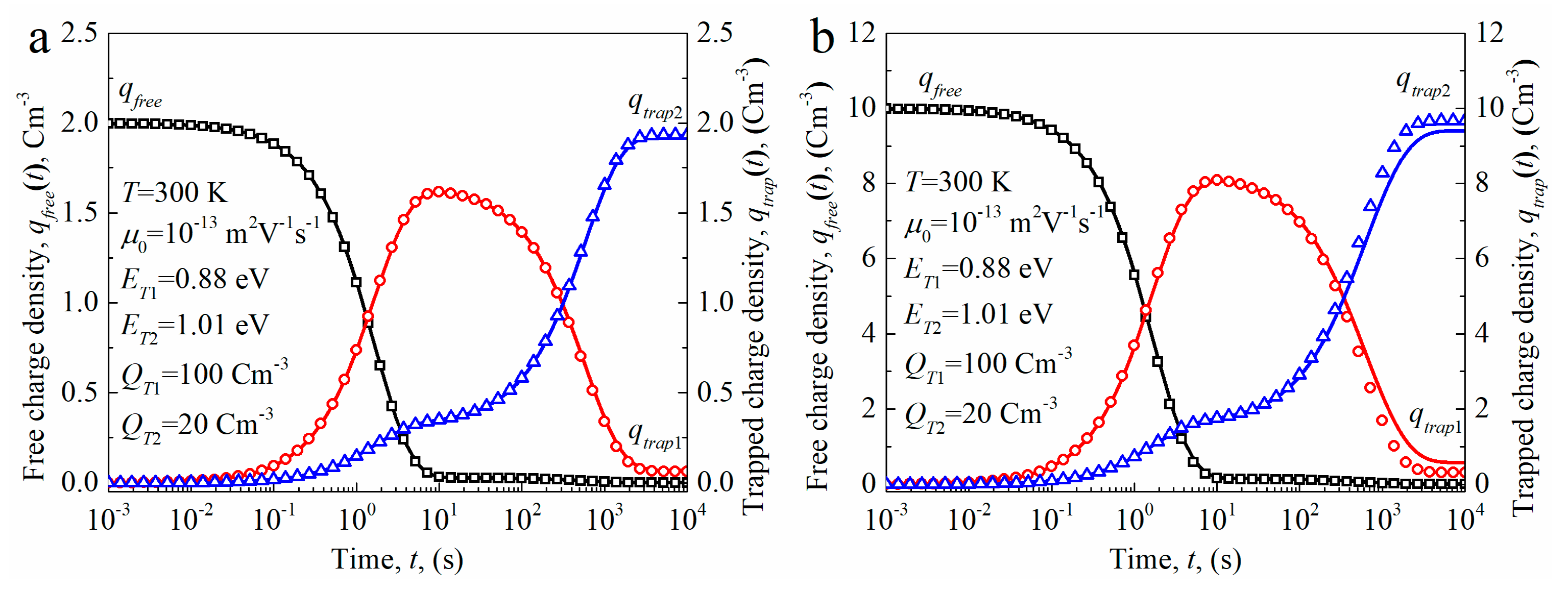
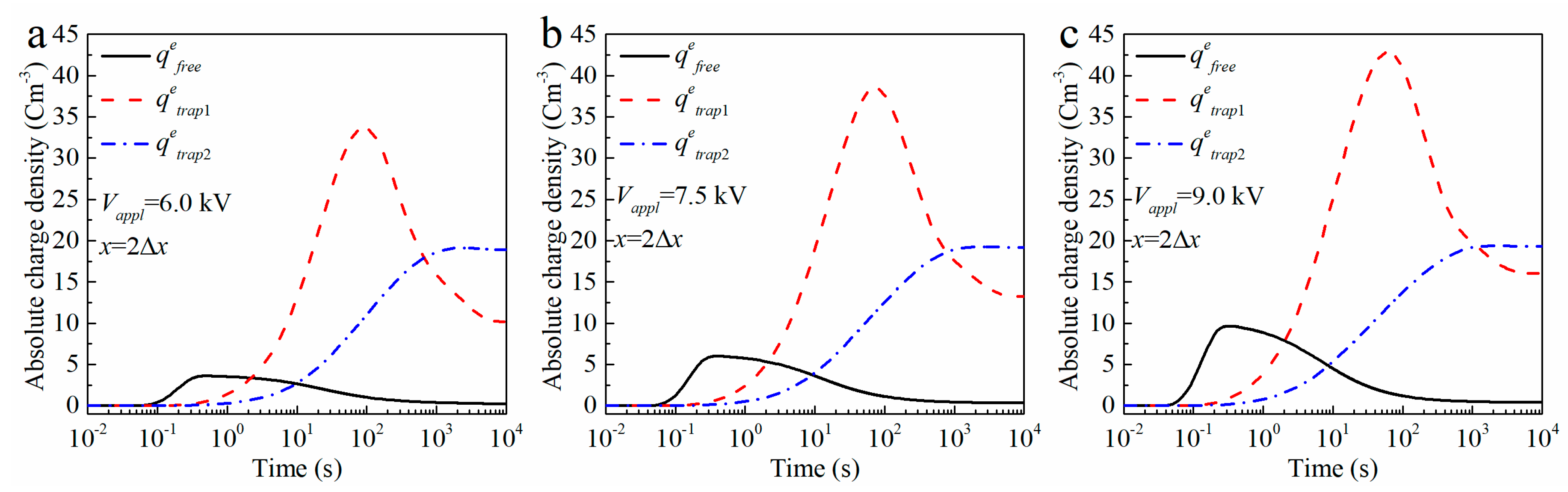
4.2. Time Dependent Free and Trapped Charge Densities at the Same Position
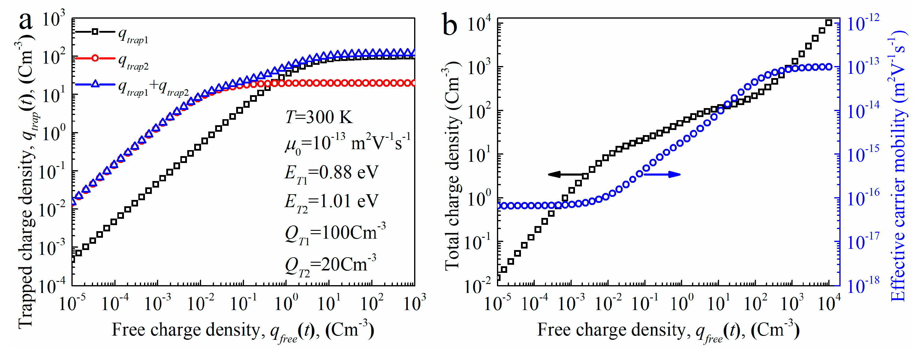
Figure 6a–c demonstrates the free and trapped charge densities as a function of time at the same position x = 2∆x in the dielectric material subjected to the voltage of 6.0 kV, 7.5 kV, and 9.0 kV, respectively. The quasi-free charges in shallow traps injected from electrodes will be captured by trap level 1 and trap level 2 simultaneously. Since the trapping probability of trap level 1 is larger than that of trap level 2, the increasing rate of trap level 1 is larger than that in trap level 2. Accordingly, significantly more charges are accumulated in trap level 1. In the meantime, the quasi-free charge density decreases with time. In addition, the charge migration and the decrease of charge injection also cause the reduction of quasi-free charges. The reduction of quasi-free charge density transfers the charge trapping/de-trapping dynamics in the case of constant quasi-free charge density to that in the case of constant total charge density. This leads to the decrease of charge density in trap level 1. The charges in trap level 1 will be transferred to trap level 2 via the transport states gradually. Finally, the charges in the material will reach thermodynamic equilibrium. At thermodynamic equilibrium, the charge densities in trap level 1 are larger than that in trap level 2 both in Figure 6.
The simulation results of charge trapping/de-trapping dynamics in dielectric materials having two discrete trap levels imply that the poling duration of applied DC voltage can influence the energy distribution properties of accumulated space charges. For short poling duration, more quasi-free charges may be captured by the trap level 1 (relatively shallower trap centers). Whereas, the trapped charges in trap level 1 will transfer to trap level 2 (relatively deeper trap centers) via the transport states for a long poling duration. The differences in the energy distribution of accumulated space charges will lead to the differences in space charge decay properties as shown in Figure 7. In the simulation model, we apply a voltage to the sample for some time (tc) and then the sample is short-circuited to simulate the space charge decay properties. When the charging time tc is 1 × 10² s, a large portion of charges are trapped in trap level 1, so the decay rate of charges after the sample is short-circuited is much higher than that with longer charging time. The same trends in the decay rate of charges were observed under the application of different voltages. After trap level 2 is fully filled, the decay rate of charges at a relatively longer time becomes the same. The charge decay properties of LDPE were investigated experimentally to demonstrate the charge trapping/de-trapping results obtained theoretically and numerically. LDPE samples with a thickness of 100 μm were charged by corona discharging for 120 s, 300 s, and 600 s at room temperature and at the humidity of 40%. The samples were charged to around −5 kV and their surface potentials were then measured by a high-voltage electrostatic voltmeter (P0865, Trek, Lockport, NY, USA) with a non-contact probe (3453ST, Trek, Lockport, NY, USA). Figure 8a shows how the surface potential decay properties change with charging time. As the charging time increases, the decay rate of surface potential decreases, because more charges are transferred into deep traps. From the surface potential decay curves, we calculated the charge densities and trap energies of LDPE. There are two discrete traps with the trap energies of 0.93 eV and 1.0 eV in the sample as shown in Figure 8b. The charge density de-trapped from shallow traps with the energy of 0.93 eV decreases with charge time, while that from deep traps increases. It indicates that during the charging process there is charge transfer from shallow traps to deep traps, so the charge decay becomes more difficult when the sample is charged for a longer time.
The charge time-dependent space charge decay behavior was also observed in XLPE [11,12] and LDPE [16,17] by PEA techniques. Tzimas et al. studied the space charge decay properties of virgin XLPE subjected to an electric field of 5 × 10⁷ Vm−1 for 2 h and 26 h at ambient temperature. The space charge distributions in the samples were measured and recorded by the PEA system. Then, the space charge density at the same position near the electrodes was extracted from the position distributions of space charges and plotted as a function of decay time. It was found that the space charge decay properties of the samples poled for various times are different. The space charges decayed slower for long poling duration. The experimental space charge decay results indicated that the charge trapping/de-trapping dynamic process of each trap center is coupled with the dynamic process of other trap centers. As shown by our analytical and numerical results in Section 2 and the BCT simulation results, the initial conditions for space charge decay processes are different for various poling durations.

4.3. Discussion

The coupling charge trapping/de-trapping dynamic processes increase the time needed for the relative deeper trap centers to reach steady states. This will prolong the periods for the energy distributions of charges to reach the thermodynamic equilibrium. Consequently, the coupling dynamics will increase the response times of transient polarization/depolarization currents, and space charge accumulation/decay processes. Therefore, the experimental results in a relatively narrow time window cannot fully interpret the charge transport behavior of polymeric dielectric materials. Montanari et al. measured the transient current densities of LDPE, XLPE, and HDPE samples at 20 °C. It was found that the transient current densities decayed for a very long time, and the steady states were not reached even after applying an electric field of 6 × 10⁷ Vm−1 for about 24 h [36]. Accordingly, the conductivities of the dielectric materials calculated from the experimental results at short poling durations would be larger than that calculated from the experimental results at long poling durations. In addition, the energy distribution of traps of XLPE evaluated from the space charge accumulation/decay experimental results at various poling durations are different.
The coupling dynamic processes will establish a dynamic equilibrium rather than a thermodynamic equilibrium in the dielectric materials [11]. It means that the traps in dielectric materials are not filled from the deepest levels upwards [22]. The traps are filled simultaneously. When the material is not in thermodynamic equilibrium, we cannot use Fermi-Dirac function (or Boltzmann function) to calculate the trapped charges density in each trap centers. Consequently, we cannot easily estimate the effective carrier mobility at transient states in the dielectric materials containing multiple discrete trap levels, the exponential energy distribution of traps, and Gaussian energy distribution of traps, etc. This means that we need to establish a novel charge transport and trapping model for dielectric materials with different types of the energy distribution of trap centers.

5. Conclusions

The space charge dynamics in LDPE with two discrete trapping centers were studied analytically and numerically. We simplified the charge trapping/de-trapping equations and obtained the analytical solutions of trapped charge densities, quasi-free charge density, and effective carrier mobility. Then, we utilized the BCT model consisting of charge injection from electrodes, charge migration in shallow traps, charge trapping, de-trapping, and recombination processes to simulate the distributions of space charges and electric fields in the material. The charge dynamic equations, charge advection equation, and Poisson’s equation in the BCT model were numerically solved by the NSFD, finite difference WENO, and BEM methods, respectively. The outputs of the BCT model showed the spatial distributions of free charge densities, trapped charge densities, and net charge densities. Charge densities at the same position in the sample as a function of time were achieved by the BCT simulations. The simulation results showed that the DC poling duration could affect the energy distribution of accumulated space charges. The charges in the relative shallower trapping centers would transfer to the relative deeper trapping centers for long poling durations. It was found that coupling dynamic processes would increase the time needed for the relative deeper trap centers to reach steady states. Therefore, experimental results for long poling duration are required to analyze the charge trapping and de-trapping properties of polymeric dielectric materials.

Author Contributions

Conceptualization, D.M.; Resources, Z.X. and Q.W.; Funding acquisition, D.M.; Writing—Original draft, D.M., H.C. and Y.H.; Writing—review & editing, Z.X., C.Z., D.M. and H.C.; Formal analysis, Z.X., C.Z.; Supervision, Q.W. and D.M.

Funding

This work was supported by State Key Laboratory of Advanced Power Transmission Technology (Grant No. GEIRI-SKL-2018-010), the National Basic Research Program of China (Grant No. 2015CB251003), the National Natural Science Foundation of China (Grant Nos. U1830131 and 51507124), and State Key Laboratory of Intense Pulsed Radiation Simulation and Effect (Northwest Institute of Nuclear Technology) (Grant No. SKIPR1709).

Conflicts of Interest

The authors declare no conflict of interest.

Appendix A

Coefficients C11, C12, C21, and C22

The initial conditions for charge trapping-de-trapping equation is assumed to be as follows:
q t r a p 1 ( t ) | t = 0 = 0 , d q t r a p 1 ( t ) d t | t = 0 = P T 1 q t o t a l
q t r a p 2 ( t ) | t = 0 = 0 , d q t r a p 2 ( t ) d t | t = 0 = P T 2 q t o t a l
Using the initial conditions for trapped charge densities and their first order derivatives, we can obtain the coefficients C11, C12, C21, and C22.
C 11 = 1 λ 1 λ 2 [ P T 1 q t o t a l + P T 1 P D 2 q t o t a l λ 2 P T 1 P D 2 + P T 2 P D 1 + P D 1 P D 2 ]
C 12 = 1 λ 1 λ 2 [ P T 1 q t o t a l + P T 1 P D 2 q t o t a l λ 1 P T 1 P D 2 + P T 2 P D 1 + P D 1 P D 2 ]
C 21 = 1 λ 1 λ 2 [ P T 2 q t o t a l + P T 2 P D 1 q t o t a l λ 2 P T 1 P D 2 + P T 2 P D 1 + P D 1 P D 2 ]
C 21 = 1 λ 1 λ 2 [ P T 2 q t o t a l + P T 2 P D 1 q t o t a l λ 1 P T 1 P D 2 + P T 2 P D 1 + P D 1 P D 2 ]

Appendix B

Relationship between qtrap1(tst) and qtrap2(tst) in the Case of Instantaneous Charge Injection

Substituting Equations (1) and (2) into Equation (21), we can obtain the exact relationship between qtrap1(tst) and qtrap2(tst).
q t r a p 1 ( t s t ) q t r a p 2 ( t s t ) = N T 1 N T 2 q t o t a l μ 0 + ε 0 ε r υ A T E exp ( E T 1 / k B T ) q t o t a l μ 0 + ε 0 ε r υ A T E exp ( E T 2 / k B T )
When qtotalμ0 << ε0εrυATEexp(−ETi/kBT), Equation (A7) approximate Equation (24).

References

  1. Teyssedre, G.; Laurent, C. Charge transport modeling in insulating polymers: From molecular to macroscopic scale. IEEE Trans. Dielectr. Electr. Insul. 2005, 12, 857–875. [Google Scholar] [CrossRef]
  2. Gao, Y.H.; Huang, X.Y.; Min, D.M.; Li, S.T.; Jiang, P.K. Recyclable Dielectric Polymer Nanocomposites with Voltage Stabilizer Interface: Toward New Generation of High Voltage Direct Current Cable Insulation. ACS Sustain. Chem. Eng. 2019, 7, 513–525. [Google Scholar] [CrossRef]
  3. Hao, J.; Zou, R.H.; Liao, R.J.; Yang, L.J.; Liao, Q. New Method for Shallow and Deep Trap Distribution Analysis in Oil Impregnated Insulation Paper Based on the Space Charge Detrapping. Energies 2018, 11, 271. [Google Scholar] [CrossRef]
  4. Wu, Y.H.; Zha, J.W.; Li, W.K.; Wang, S.J.; Dang, Z.M. A remarkable suppression on space charge in isotatic polypropylene by inducing the beta-crystal formation. Appl. Phys. Lett. 2015, 107, 112901. [Google Scholar] [CrossRef]
  5. Chen, G.; Tay, T.Y.G.; Davies, A.E.; Tanaka, Y.; Takada, T. Electrodes and charge injection in low-density polyethylene - Using the pulsed electroacoustic technique. IEEE Trans. Dielectr. Electr. Insul. 2001, 8, 867–873. [Google Scholar] [CrossRef]
  6. Mizutani, T. Space-Charge Measurement Techniques and Space-Charge in Polyethylene. IEEE Trans. Dielectr. Electr. Insul. 1994, 1, 923–933. [Google Scholar] [CrossRef]
  7. Zha, J.W.; Dang, Z.M.; Song, H.T.; Yin, Y.; Chen, G. Dielectric properties and effect of electrical aging on space charge accumulation in polyimide/TiO2 nanocomposite films. J. Appl. Phys. 2010, 108, 094113. [Google Scholar] [CrossRef]
  8. Blaise, G. Space-Charge Physics and the Breakdown Process. J. Appl. Phys. 1995, 77, 2916–2927. [Google Scholar] [CrossRef]
  9. Wu, K.; Dissado, L.A.; Okamoto, T. Percolation model for electrical breakdown in insulating polymers. Appl. Phys. Lett. 2004, 85, 4454–4456. [Google Scholar] [CrossRef]
  10. Jones, J.P.; Llewellyn, J.P.; Lewis, T.J. The contribution of field-induced morphological change to the electrical aging and breakdown of polyethylene. IEEE Trans. Dielectr. Electr. Insul. 2005, 12, 951–966. [Google Scholar] [CrossRef]
  11. Tzimas, A.; Rowland, S.M.; Dissado, L.A.; Fu, M.; Nilsson, U.H. The effect of dc poling duration on space charge relaxation in virgin XLPE cable peelings. J. Phys. D Appl. Phys. 2010, 43, 215401. [Google Scholar] [CrossRef]
  12. Tzimas, A.; Rowland, S.M.; Dissado, L.A. Effect of Electrical and Thermal Stressing on Charge Traps in XLPE Cable Insulation. IEEE Trans. Dielectr. Electr. Insul. 2012, 19, 2145–2154. [Google Scholar] [CrossRef]
  13. Many, A.; Rakavy, G. Theory of Transient Space-Charge-Limited Currents in Solids in the Presence of Trapping. Phys. Rev. 1962, 126, 1980–1988. [Google Scholar] [CrossRef]
  14. Le Roy, S.; Baudoin, F.; Griseri, V.; Laurent, C.; Teyssedre, G. Charge transport modelling in electron-beam irradiated dielectrics: A model for polyethylene. J. Phys. D Appl. Phys. 2010, 43, 315402. [Google Scholar] [CrossRef]
  15. Toomer, R.; Lewis, T.J. Charge Trapping in Corona-Charged Polyethylene Films. J. Phys. D Appl. Phys. 1980, 13, 1343–1356. [Google Scholar] [CrossRef]
  16. Chen, G.; Xu, Z.Q. Charge trapping and detrapping in polymeric materials. J. Appl. Phys. 2009, 106, 123707. [Google Scholar] [CrossRef] [Green Version]
  17. Zhou, T.C.; Chen, G.; Liao, R.J.; Xu, Z.Q. Charge trapping and detrapping in polymeric materials: Trapping parameters. J. Appl. Phys. 2011, 110, 043724. [Google Scholar] [CrossRef] [Green Version]
  18. Mizutani, T.; Suzuoki, Y.; Hanai, M.; Ieda, M. Determination of Trapping Parameters from Tsc in Polyethylene. Jpn. J. Appl. Phys. 1982, 21, 1639–1641. [Google Scholar] [CrossRef]
  19. Liang, H.C.; Du, B.X.; Li, J.; Li, Z.L.; Li, A. Effects of non-linear conductivity on charge trapping and de-trapping behaviours in epoxy/SiC composites under DC stress. IET Sci. Meas. Technol. 2018, 12, 83–89. [Google Scholar]
  20. Gao, Y.; Wang, J.L.; Liu, F.; Du, B.X. Surface Potential Decay of Negative Corona Charged Epoxy/Al2O3 Nanocomposites Degraded by 7.5-MeV Electron Beam. IEEE Tran. Plasma Sci. 2018, 46, 2721–2729. [Google Scholar] [CrossRef]
  21. Meunier, M.; Quirke, N.; Aslanides, A. Molecular modeling of electron traps in polymer insulators: Chemical defects and impurities. J. Chem. Phys. 2001, 115, 2876–2881. [Google Scholar] [CrossRef]
  22. Boufayed, F.; Teyssedre, G.; Laurent, C.; Le Roy, S.; Dissado, L.A.; Segur, P.; Montanari, G.C. Models of bipolar charge transport in polyethylene. J. Appl. Phys. 2006, 100, 104105. [Google Scholar] [CrossRef] [Green Version]
  23. Kuik, M.; Koster, L.J.A.; Wetzelaer, G.A.H.; Blom, P.W.M. Trap-Assisted Recombination in Disordered Organic Semiconductors. Phys. Rev. Lett. 2011, 107, 256805. [Google Scholar] [CrossRef] [PubMed] [Green Version]
  24. Kuik, M.; Koster, L.J.A.; Dijkstra, A.G.; Wetzelaer, G.A.H.; Blom, P.W.M. Non-radiative recombination losses in polymer light-emitting diodes. Org. Electron. 2012, 13, 969–974. [Google Scholar] [CrossRef] [Green Version]
  25. Vonberlepsch, H. Interpretation of Surface-Potential Kinetics in Hdpe by a Trapping Model. J. Phys. D Appl. Phys. 1985, 18, 1155–1170. [Google Scholar] [CrossRef]
  26. Le Roy, S.; Teyssedre, G.; Laurent, C.; Montanari, G.C.; Palmieri, F. Description of charge transport in polyethylene using a fluid model with a constant mobility: Fitting model and experiments. J. Phys. D Appl. Phys. 2006, 39, 1427–1436. [Google Scholar] [CrossRef]
  27. Tian, J.H.; Zou, J.; Wang, Y.S.; Liu, J.; Yuan, J.S.; Zhou, Y.X. Simulation of bipolar charge transport with trapping and recombination in polymeric insulators using Runge-Kutta discontinuous Galerkin method. J. Phys. D Appl. Phys. 2008, 41, 195416. [Google Scholar] [CrossRef]
  28. Simmons, J.G.; Taylor, G.W. Nonequilibrium Steady-State Statistics and Associated Effects for Insulators and Semiconductors Containing an Arbitrary Distribution of Traps. Phys. Rev. B 1971, 4, 502–511. [Google Scholar] [CrossRef]
  29. Chapwanya, M.; Lubuma, J.M.S.; Mickens, R.E. Nonstandard finite difference schemes for Michaelis-Menten type reaction-diffusion equations. Numer. Meth. Part. Differ. Equ. 2013, 29, 337–360. [Google Scholar] [CrossRef]
  30. Min, D.M.; Wang, W.W.; Li, S.T. Numerical Analysis of Space Charge Accumulation and Conduction Properties in LDPE Nanodielectrics. IEEE Trans. Dielectr. Electr. Insul. 2015, 22, 1483–1491. [Google Scholar] [CrossRef]
  31. Li, S.T.; Min, D.M.; Wang, W.W.; Chen, G. Modelling of Dielectric Breakdown through Charge Dynamics for Polymer Nanocomposites. IEEE Trans. Dielectr. Electr. Insul. 2016, 23, 3476–3485. [Google Scholar] [CrossRef]
  32. Sessler, G.M.; Figueiredo, M.T.; Ferreira, G.F.L. Models of charge transport in electron-beam irradiated insulator. IEEE Trans. Dielectr. Electr. Insul. 2004, 11, 192–202. [Google Scholar] [CrossRef]
  33. Jiang, G.S.; Shu, C.W. Efficient implementation of weighted ENO schemes. J. Comput. Phys. 1996, 126, 202–228. [Google Scholar] [CrossRef]
  34. Le Roy, S.; Teyssedre, G.; Laurent, C. Numerical methods in the simulation of charge transport in solid dielectrics. IEEE Trans. Dielectr. Electr. Insul. 2006, 13, 239–246. [Google Scholar] [CrossRef]
  35. Cockburn, B.; Shu, C.-W. TVB Runge-Kutta Local Projection Discontinuous Galerkin Finite Element Method for Conservation Laws II: General Framework. Math. Comput. 1988, 52, 411–435. [Google Scholar]
  36. Montanari, G.C.; Mazzanti, G.; Palmieri, F.; Motori, A.; Perego, G.; Serra, S. Space-charge trapping and conduction in LDPE, HDPE and XLPE. J. Phys. D Appl. Phys. 2001, 34, 2902–2911. [Google Scholar] [CrossRef]
Figure 1. Schematic dynamics of charge trapping/de-trapping events in dielectric materials containing two discrete levels of traps for (a) continuous charge injection and (b) instantaneous charge injection. Here EC is the conduction band, ET1 and ET2 the energies of traps, EF the Fermi level, PT1 and PT2 the trapping probabilities for free charges, and PD1 and PD2 the de-trapping probabilities of trapped charges.
Applsci 09 04253 g001
Figure 2. Time-dependent free charge density and trapped charge densities in the dielectric material containing two discrete trap levels in the case of instantaneous charge injection. The total charge densities are 2 cm−3 (a) and 10 cm−3 (b). Solid lines are numerical results, and dots are analytical results.
Applsci 09 04253 g002
Figure 3. Trapped charge densities (a) and total charge density and effective carrier mobility (b) as a function of free charge density at steady state in dielectric materials containing two discrete trap levels.
Applsci 09 04253 g003
Figure 4. Schematic of bipolar charge transport model of dielectric materials containing two discrete traps. Here ETe1 and ETe2 are the two discrete deep traps of electrons, while ETh1 and ETh2 are the two discrete deep traps of holes.
Applsci 09 04253 g004
Figure 5. Average net space charge densities (a) and external current densities (b) as a function of time in the dielectric material containing two discrete trap levels subjected to various voltages.
Applsci 09 04253 g005
Figure 6. Time dependent free charge density and trapped charge densities at the same position x = 2∆x in the dielectric material subjected to the voltage of 6.0 kV (a), 7.5kV (b), and 9.0kV (c).
Applsci 09 04253 g006
Figure 7. Space charge decay properties at the same position in the dielectric material charged for various times under the voltages of 6.0 kV (a), 7.5 kV (b), and 9.0 kV (c).
Applsci 09 04253 g007
Figure 8. Surface potential decay curves of low-density polyethylene samples after charging by corona discharging for different times (a) and the de-trapped charge density as a function of trap energy calculated from surface potential decay experimental results (b).
Applsci 09 04253 g008
Table 1. The assigned parameter values used in the charge trapping/de-trapping dynamic analysis.
ParameterValue
Charge carrier mobility, μ0, (m2 V−1 s−1)1.0 × 10⁻¹³
Energy of trap level 1, ET1, (eV)0.88
Energy of trap level 2, ET2, (eV)1.01
Charge density of trap level 1, QT1, (cm−3)100
Charge density of trap level 1, QT2, (cm−3)20

