Abstract
This paper reviews the state of the art in offshore wind farm operations and maintenance with a focus on decision support models for the scheduling of maintenance. Factors influential to maintenance planning are collected from the literature and their inclusion in state-of-the-art models is discussed. Methods for modeling and optimization are presented. The methods currently used and possible alternatives are discussed. The existing models are already able to aid the decision-making process. They can be improved by applying more advanced mathematical methods, including uncertainties in the input, regarding more of the influential factors, and by collecting, analyzing, and subsequently using more accurate data.
1. Introduction
The demand for energy from offshore wind parks is rising and the offshore wind industry is growing fast [1,2,3]. Currently, up to a third is the cost of energy can be attributed to maintenance cost [4]. In the last decade a rising number of researchers has been working on approaches to lower these costs. Condition monitoring can give a better overview of the turbine status and increase the detection rate of failures before they occur. Preventive maintenance can then stop these failure failures from happening, reducing unexpected downtime. Also, the strategy of how to handle unexpected failures and corrective maintenance has been the focus of research.
Many factors, such as probability of failures and weather conditions, influence the choice of maintenance strategy and including all of them when taking an informed decision can be challenging for human decision makers. A decision support system can be used to facilitate the choice. Decision support systems (DSS) arose shortly after the invention of modern computers and are now used across industries. Power [5] presents a brief history of the development of DSS from the 1960s to the early 2000s. Early definitions of DSS were broad and included any type of computerized system to aid human decision makers. Over time, different branches of decision support emerged. In Kessler [6], David L. Olsen summarized five types of DSS presented by Power [5]. These are communication-driven, data-driven, document-driven, knowledge-driven, and model-driven DSS. A communication-driven DSS supports the communication, when multiple people work together on a task. Data-driven DSS focus on data access and the use and manipulation of data. In document-driven DSS text manipulation is in focus, managing unstructured information. Knowledge-driven DSS present expertise in form of rules or procedures. This often overlaps with communication- and document-driven DSS. Model-driven DSS highlight statistical or operation research modeling. In the case of offshore wind farm operations and maintenance scheduling, model-driven decision support can be used.
In this review article, we present the current state of the art in operations and maintenance decision support research for offshore wind farms. In their review of operation and maintenance of wind power assets El-Thalji and Liyanage [7] observe that the main academic contributions in the field are on condition monitoring, diagnostics, and prognostics. During the literature research for this paper, the present authors have gotten the same impression of the field. We do not want to exclude condition monitoring from our analysis. However, the aim is to focus on maintenance scheduling in the present paper. Hofmann [8] has presented a review of decision support models for operation and maintenance planning in 2011. With this review we want to cover the development since 2011 and focus on the modeling details. In Section 2 we explore which factors are influential to the decision. The individual factors, how they are considered in recent literature and how the decision support tools model these factors are discussed in Section 2.1, Section 2.2, Section 2.3, Section 2.4 and Section 2.5. The maintenance strategy and different kinds of maintenance are discussed in Section 3. Different modeling techniques are investigated in Section 4, this includes methods currently used in decision support models for offshore wind farm maintenance scheduling. Section 5 reviews optimization techniques and discusses those techniques currently used in maintenance scheduling models for offshore wind farms. The availability of data and data used in the existing models and tools are discussed and presented in Section 6 before we discuss the results in Section 7 and conclude the paper in Section 8. Throughout the paper, references to the literature are ordered chronologically first and alphabetically within the year of publication.
2. Operation and Maintenance: Influential Factors
When scheduling maintenance for offshore wind farms, many different factors need to be considered. Many different researchers analyzed the influences on the maintenance and presented similar results. According to most publications, the factors influencing the planning and cost of maintenance are the occurrence of failures, availability of maintenance crew, spare parts and vessels, weather and external factors, the chosen maintenance strategy, and economical parameters such as the electricity price and subsidies. While laws and legal restrictions also influence the operation of offshore wind farms, they are only included in the models in form of working-hour restrictions and often not included at all. This is possibly due to the fact, that a wind farm maintenance provider or operator cannot wield influence on these factors. Table 1 summarizes the factors mentioned by the different authors.

Table 1.
This is a table summarizing the factors influential to the offshore wind farm operation and maintenance scheduling.
In the following subsections, we comment on the individual influencing factors presented in the literature. First, we investigate the modeling of degradation and failures. Next, we discuss the availability of maintenance supply, such as crew, vessels, and spare parts. Then, the routing of vessels and transportation are discussed. Subsequently, weather modeling, the uncertainty in weather and forecasts is presented. Finally, this is followed by economical parameters and cost estimation.
2.1. Degradation and Failure Modeling
The occurrence of a failure in a wind turbine in a wind farm gives rise to a necessary repair and forms the cause of any maintenance action. Since the occurrence of a failure directly causes maintenance actions and is therefore the reason for the connected costs, the existing analyses are concerned with the probability and frequency of failure occurrence. The main difference between different tools/models is the way the failures are presented. In some of the publications, historic operational data is used to estimate the failure behavior. In some cases, failures are assumed to occur after a certain amount of time, the occurrence of failures is therefore modeled in a deterministic way. The mean time between failure (MTBF) can be calculated from observed failures and is often used for this deterministic modeling. In other models, failures occur with a certain probability that is assessed based on collected data, so the failures are occurring randomly according to a defined probability distribution. To model from this probability distribution, samples are drawn from the distribution(s). Popular processes for failure distribution modeling are (homogeneous) Poisson processes (In a Poisson process, the probability of having a certain number n of (failure) occurrences N(t) at time t is: ), where the time intervals between failures are exponentially distributed, according to a given failure rate . In some models, the failure rate can be updated, leading to an inhomogeneous Poisson process, with a failure rate function . Other distributions that are being used to sample the time between failures are the Weibull distribution (the Weibull distribution is a continuous probability distribution with density function ), Gamma process (A Gamma process is a stochastic process, comprised of increments that are independently Gamma distributed, with density functions: where is the Gamma function.) and Bernoulli process (A Bernoulli process is a discrete stochastic process taking two different values and is comprised of a sequence of binary random variables). A summary of the different methods used to model degradation and failures in the literature is presented in Table 2.
Table 2.
This table summarizes the methods used for degradation and failure modeling presented in the literature.
2.2. Vessel, Personnel and Spare Part Logistics
To repair the defects and failures occurring in the offshore wind farm, there are three main requirements. The availability of maintenance workers that are trained to conduct the respective maintenance tasks is crucial. Many repairs need not only a repair team and tools, but also specific spare parts. The availability of those poses another restriction to performing the maintenance and should therefore be included in any maintenance model. To transport both workers and spare parts to the offshore location, transport vessels are required. Therefore, the availability of those presents another part of maintenance analysis and should be included in any model. Additional to the transport vessels, some repairs require jack-up barges or crane vessels. This includes gearbox replacements and blade repair. Most existing models include at least one of the factors.
Scheu et al. [12] consider in their decision support model two different vessel types, with specific weather restrictions. Additionally, the crew size varies for different turbine components and each vessel has a fixed crew capacity. Besnard et al. [13] present a model for an offshore wind farm. With this model, they optimize the number of maintenance technicians, length of shifts, location of accommodation and the choice of transfer vessels and helicopters. In the presented case study, an offshore accommodation with technicians available at any time was favored. For the optimal transport of the workers to the turbines, a crew transfer vessel with an improved access system was chosen. To find the optimal vessel fleet size and composition is the goal of Halvorsen-Weare et al. [15]. They present a mixed-integer program and compare 15 different instances. Hofmann and Sperstad [16] consider different combinations of vessel types, with different abilities and access restrictions, as well as different ownership models (purchasing the vessel, chartering the vessel). Spare parts are always considered available, with a fixed lead-time and cost. In the logistics module of Asgarpour and van de Pieterman [31] an equipment analysis, spare part analysis and repair class analysis is included. Endrerud et al. [17] include a deterministic waiting time for spare parts depending on the failure type. The number of technicians and vessels needed is also determined by the failure type. Only one type of technicians is considered. Three different vessel types can be chosen in the model, with different charter contracts. In Sperstad et al. [19] a deterministic optimization of the vessel fleet size and the decision whether to purchase or charter vessels is presented. They also consider different locations for the maintenance base. In their model, Dalgic et al. [20] consider four different transportation systems, a crew transfer vessel, a helicopter, an offshore access vessel and a jack-up vessel. Each system has a specific maximum number of workers it can carry as well as type specific access restrictions, travel times and mobilization costs. The shift length for the maintenance workers is 12 hours. Each worker can only be assigned to one turbine per shift. Endrerud and Liyanage [21] is based on Endrerud et al. [17] and the number of technicians and vessels needed as well as the wait time for spare parts is determined by the failure type. In Sahnoun et al. [22] the availability of vessels, spare parts and cranes is considered. The personnel are divided into electricians and technicians and the availability of spare parts in unlimited. A review of the organization of maintenance logistics was done by Shafiee [43]. He classifies the spare parts inventory management and the maintenance support organization (vessels, cranes, helicopters, personnel) as a tactical issue in offshore wind farm maintenance logistics. Gintautas and Sørensen [24] present constraints for both installation and O&M vessels given in the previous literature by Dinwoodie et al. [44], Besnard et al. [13], Nielsen and Sørensen [10], O’Connor et al. [45], Van Bussel and Bierbooms [46], O’Connor et al. [47], McMillan and Ault [48], Wu [49] and Ahn et al. [50]. Raknes et al. [25] consider two different vessel types—an accommodation vessel and a crew transfer vessel, in their analysis. The vessels vary in properties, such as capacity and weather conditions. Rinaldi et al. [26] consider the spares in stock and a procurement time as well as different types and numbers of vessels, both rented and purchased in their model. The model also allows for helicopters to be used.
2.3. Transportation and Vessel Routing
In addition to the availability of crew, spare parts and vessels, the transport of crew and parts to the offshore wind turbine must be organized. Therefore, a route must be established for the vessels to unload and pick-up crew and parts. Those tasks requiring a vessel or crane at the turbine need to be scheduled in the vessels route as well.
Van Bussel and Bierbooms [46] analyzed the transport of crew and small parts for the DOWEC reference wind farm [51]. They combine five different vessel types and four different maintenance categories. Their simulation shows that high availability can be achieved for a hard to access farm, by optimizing the access system and maintenance strategy. Three different transport options are considered by Nielsen and Sørensen [10]. The simplest option is to always access the wind turbines with a boat if a repair needs to be conducted. Option two is to conduct the repair as soon as possible, using a helicopter if access with a boat is restricted due to waves. The third option is to do a risk-based analysis to determine the transport alternative. Here the cheapest solution, including production losses, is calculated based on a weather forecast that is assumed to be perfect. Halvorsen-Weare et al. [52] investigate fleet composition and vessel routing for offshore oil and gas industries. Their optimization model provides weekly routes and schedules for the vessels. Since offshore wind turbine maintenance vessels differ from offshore supply vessels and since the needs for corrective maintenance and immediate access are hard to plan very far ahead, the model needs to be modified to solve vessel routing problems for offshore wind. Hofmann and Sperstad [16] do not model the vessel routing but consider a fixed travel time for each vessel type from the maintenance base to the wind farm instead. In Endrerud et al. [17] and Endrerud and Liyanage [21], vessels travel the shortest distance between their location and destination. A vessel specific speed is used to calculate the travel times. However, no optimization of the routing takes place. Sperstad et al. [19] compare different access restriction for the vessel routing. They use both single- and multi-criteria restrictions and show that a single value limit (significant wave height) is sufficient, as long as the value is estimated in a correct way. Dalgic et al. [20] consider three types of transportation, with a different routing plan each. For the crew transfer vessels and helicopters, the first mobilized transport system is routed such that the number of turbine visits is maximized, while minimizing the total number of vessels/helicopters used. The workers are dropped off at the turbines and later collected, such that the vessel/helicopter is free to travel within the wind farm during the shift. Tasks that can be completed within one shift are prioritized. The offshore access vessel visits the turbines sequentially and stays at the turbine while the maintenance is conducted, it is only limited by daylight and weather restrictions. Also, the jack-up vessel visits the turbines that need maintenance in sequence and is limited by weather restrictions. Halvorsen-Weare and Fagerholt [53] present two models for solving the offshore supply vessel routing and scheduling problem. As for the model in Halvorsen-Weare et al. [52], modifications are necessary to apply the models to offshore wind. Martini et al. [54] present an accessibility analysis for the North Sea. They investigate two different vessel types and present the access restrictions for them. Raknes et al. [25] present a vessel routing and maintenance scheduling model. They compare different vessel fleet compositions with a commercial mixed-integer programming solver and two rolling-horizon heuristics. In their model Rinaldi et al. [26] consider a mobilization and a response time for the vessels as well as operational limits for the vessels and restrictions for overnight work. Therefore, they also include a model to calculate the sunrise and sunset times for each day. Schrotenboer et al. [55] present a two-stage adaptive large neighborhood search to solve the technician allocation and routing problem. The optimization presented by Stock-Williams and Swamy [41] aims to find the optimal daily maintenance vessel routing and repair schedule.
2.4. Weather and External Factors
Rothkopf et al. [56] present a Markovian wave height model that uses tri-diagonal transition matrices. This model can be used in any Monte Carlo simulation for offshore simulations. Anastasiou and Tsekos [57] present a study on the persistence of different marine environmental parameters based on Markov theory. They assume that the process governing the distribution of the persistence of marine environmental conditions can be regarded as a stationary first order Markov process. The transition matrix for this Markov process can be established from recorded weather data. They use a discrete time Markov chain and compare the transition matrix of the original Markov process with a simplified two-by-two matrix with transition probabilities from below and above a certain threshold. According to their investigations, six to eight different states in the Markov model are sufficient to adequately model the marine environmental parameters. Finally, they also show that the Markov model has a better performance than the Kuwashima-Hogben model [58] in terms of persistence distribution. Monbet and Marteau [59] present a continuous-space discrete time Markov model of higher order to model significant wave height peak period and wind speed. The Markov model can be used to generate new sequences of the time series. Lange [60] investigated the uncertainty of wind speed forecasts and found that the statistical distribution of the prediction errors (deviation between predicted and measured wind speed) is Gaussian. Dinwoodie et al. [11] use autoregressive (AR) models to model both the wave height and wind speed. For the wind speed an AR model of order 2 is used and for the wave heights an AR model of order 20 is used. To use these AR models some transformations of the data must be conducted. For the wind speed, a fit of the monthly mean and diurnal variations must be removed. For the significant wave height, a fit of the monthly means is removed, and a Box-Cox transformation is applied. Douard et al. [30] use a hidden Markov model (HMM) to calculate the waiting time for each failure. This HMM calculates the waiting time based on meteorological site characteristics, seasonality is respected, the HMM is robust to model uncertainty and the variability in the meteorological site conditions is preserved. Scheu et al. [12] on the other hand use a discrete time Markov chain model to generate time series of the wave height. The wind speed is generated according to a correlation matrix. Dinwoodie et al. [14] use a multivariate autoregressive time series to model correlated wind speeds and wave heights. Feuchtwang and Infield [61] calculate the maintenance delays due to sea state with a closed form probabilistic model. In their model, they consider access restrictions and a Weibull distribution for the weather, fitted to represent the conditions of a given site. Hagen et al. [62] present a multivariate Markov model to generate sea state time series. The sea state is a combination of wind speed, wind direction, wave height, wave direction and wave period. They present two ways of capturing the seasonal variation within the sea state. The first method is to use monthly models assuming piece-wise stationarity. The second model uses a data transformation to deal with the seasonal variation. In their simulation model, Hofmann and Sperstad [16] use a Markov chain process to simulate weather time series. They assume a perfect weather forecast for the duration of the next shift. The met ocean module from Asgarpour and van de Pieterman [31] uses re-sampling of wind and wave data and provides wind shear model parameters as well as operational limits for each equipment type in addition to the time series for wind speed and significant wave height. Endrerud et al. [17] use significant wave height and wind speed at hub height in hourly resolution as input to their model. The only uncertainty is therefore the variation within the given data. For the simulation of the weather in the model Sperstad et al. [19] use the simulation model from Hofmann and Sperstad [16]. Dalgic et al. [20] also use a multivariate autoregressive model to generate synthetic weather. They use sea level wind speeds for the access restrictions and hub height wind speeds for the maintenance with a jack-up vessel and for production. For the wave climate, wave heights and wave periods are used. With this model, they maintain the persistence, seasonality and correlation between wind speed, wave height and wave period of the site-specific weather. Endrerud and Liyanage [21], such as Endrerud et al. [17] use the significant wave height and wind speed at hub height as input. Joschko et al. [33] in their simulation of offshore wind farm O&M processes use stochastic weather. The weather is generated inside the model according to a distribution that is taken from actual wind farm data. As an influence on the production and degradation wind speed, wave height, lightning and visibility are used Sahnoun et al. [22]. Abdollahzadeh et al. [34] take into account only the wind speeds at the location of the wind farm and model these according to a Weibull distribution. Ambühl et al. [63] model the uncertainty in the weather forecast by adding an error term to the weather forecast to calculate the actual weather, using the knowledge about normally distributed errors from Lange [60]. Gintautas and Sørensen [24] base their weather window predictions on weather forecasts and an acceptance criteria exceedance event formulation and present two case studies. The uncertainty in the weather conditions in this case stems directly from the uncertainty in the weather forecasts. They achieve a prediction of longer weather windows with their improved model. Hersvik and Endrerud [64] present a weather series generator using a piece-wise Markov chain process. In their model, there exists no transition probability matrix, but instead a piece of the original time series of random length is copied from a random place in the time series with the same transition between weather states. The model includes seasonality by looking at the current month for a transition first and only looks outside of the current month if the specific transition cannot be found there. The benefit of using piece-wise copies of the original time series is the high detail level in the generated time series that is lost, when transition probabilities between weather states are used. Martini et al. [54] presented a new approach to wind farm accessibility. In addition to previous accessibility studies, they also include spatial variability in wind speeds and wave heights. Their accessibility analysis is conducted for long-term accessibility and in high resolution. The model in Rinaldi et al. [26] uses time series as an input and requires a minimum weather window to conduct maintenance. A stochastic process for weather generation has been presented and investigated by Seyr and Muskulus [65]. The advantage of this method is that it can be used as an alternative to simulation-based generation models. Taylor and Jeon [66] present approaches of probabilistic forecasting of the wave height. The presented approaches are ARMA-GARCH models that might be applied to decision-making in the future as an alternative to other forecasting methods.
2.5. Economic Parameters and Cost Estimation
The goal of effective maintenance scheduling will be the maximizing of economic profit. Therefore, economical parameters such as electricity price or feed-in-tariff (FIT), cost of vessel hire, cost of spare parts and worker salaries are an important input to maintenance modeling. While electricity price or FIT are usually used to calculate the profits of a wind farm or electricity costs for other industries, when used in maintenance models, it is used to calculate the production loss from turbine downtime. Vessel hire, worker costs and cost of spare parts have a direct influence on the maintenance costs. Many models include fixed rates for the vessel hire, worker and spare part costs, while some of the existing models try to include variable vessel and worker costs.
Dinwoodie et al. [11] mention two ways to calculate the production loss. The basic method is to use the rated power of the turbine and multiply it by a capacity factor and length of downtime. A more accurate approach is to use a time series of the wind speed and determine the lost revenue from a power curve. In addition to the lost revenue, also costs due to vessel and staff hire, and component replacement must be considered. In Douard et al. [30] the cost estimation has both a deterministic and a probabilistic part. The deterministic part includes the capital cost, operational costs for fixed and preventive maintenance as well as the monitoring of the turbines. The probabilistic cost is corrective maintenance and condition-based maintenance which depend on the failure rates. Both deterministic costs and probabilistic costs include direct and indirect costs. The direct costs include the labor, transport, spare parts costs, and indirect costs being caused by the downtime (dependent on the maintenance duration) and the waiting time (dependent on the weather). Scheu et al. [12] focus in their decision support model on the production losses due to downtime. They are calculated by using a linearized power curve, the wind speed, and a FIT for the UK. Dinwoodie et al. [14] estimate cost distributions for different maintenance scenarios. They base the cost estimation on four different vessel charter scenarios, with different charter rates. Additionally, they include fixed mobilization costs and seasonality of the costs. The cost distribution is then derived via regression analysis. Hofmann and Sperstad [16] present the net present O&M costs including spare part and consumable costs, vessel costs, personnel costs as well as cost for using locations such as harbor and costs for transporting personnel to locations such as mother ships and offshore platforms. In addition to the net present O&M cost they also present the net present value of profit and the net present income based on electricity production. Asgarpour and van de Pieterman [31] present in their report the operation and maintenance cost estimator project by ECN. The cost estimator includes the operation and maintenance, logistics as well as met ocean modules. Endrerud et al. [17] include generic repair and replacement costs as well as vessel day rates, salary costs, warehousing costs, overhead costs, spare part costs, rent, taxes and insurance in their decision support model. They encourage the user to provide more accurate data to get a more accurate output, i.e., lost production and marine logistics cost, that is generated by the simulation. Dalgic et al. [20] in their analysis consider electricity price, fixed vessel cost, vessel charter costs, technician costs, fuel cost, cost of preventive maintenance, component repair cost and insurance cost. They use different costs for helicopters, crew transfer, offshore access and jack-up vessels and report the numbers used as input in their analysis. Endrerud and Liyanage [21] is based on Endrerud et al. [17] and the same costs are included. Sahnoun et al. [22] consider maintenance action costs, the energy cost, installation of monitoring systems. The costs depend on the failure type, the maintenance type the maintenance duration, weather conditions during the maintenance action and the cost of maintenance facilities as given from Nilsson and Bertling [67] as well as considering the production losses. Asgarpour and Sørensen [36] use the ECN O&M tool from Rademakers et al. [68] in their case study to estimate the total O&M costs. They consider all costs associated with inspection, monitoring, maintenance activities and revenue loss due to downtime and calculate the cost for each possible outcome in their decision tree. Shafiee et al. [23] consider in their cost model operation costs including rental payments, insurance, and transition charges (grid), as well as maintenance costs including both direct (transport of components, technicians, consumables, and spare parts) and indirect (port fees, weather forecast) maintenance costs. Rinaldi et al. [26] consider replacement costs for spare parts.
3. Maintenance Strategy
Shafiee [43] presents three different categories of issues in offshore wind farm maintenance planning. These are technical, strategic, and operational issues. The technical issues are covered by the failures. Operational issues are comprised of availability of vessels, crew, and spare parts, the weather and other external and economic factors. For the strategical issues, choosing the optimal maintenance strategy is the challenge wind farm operators are facing in their work. Therefore, any maintenance scheduling model should be able to incorporate and evaluate different maintenance strategies. Most models compare some fixed input scenarios or optimize certain aspects of the strategy, such as fleet size and grouping of repairs. All these approaches have the drawback that the operator or researcher using the model must already have an idea of how the maintenance can be improved and be familiar with the factors that influence the scheduling of maintenance. A maintenance model that can also optimize the maintenance strategy without input from the operator or a researcher, does not yet exist. However, since a well-developed model could be used by persons who are not familiar with the problems of offshore maintenance scheduling, the development of such a model is highly encouraged. Krokoszinski [69] wrote that an optimal O&M strategy should strive to maximize the total overall equipment effectiveness, which is the product of the planning factor and the overall equipment effectiveness. The overall equipment effectiveness is the factor between the valuable production time and available production time (equal to productivity). The total overall equipment effectiveness is the actually valuable production time with respect to the theoretical production time, so it includes e.g., downtime losses.
An overview over the different models and which kinds of maintenance they include is presented in Table 3. More details about the different kinds of maintenance are presented in the following subsections.
Table 3.
This table summarizes the use of different types of maintenance in the literature.
3.1. Preventive Maintenance
Preventive maintenance is a kind of maintenance that is conducted pro-actively before the occurrence of a fault or failure. Without any prior knowledge of the timing of failures, preventive maintenance is planned to be conducted in a fixed time interval. Preventive maintenance can return a (degrading) component to an “as-good-as-new” state or lower the degradation by a fixed amount. Different models include preventive maintenance in different ways.
Van Bussel and Bierbooms [46] include regular preventive maintenance tasks in their model. Hofmann and Sperstad [16] consider time-based preventive maintenance in their model, defined by a fixed time interval, returning a components state back to its original value. Shafiee and Finkelstein [32] investigate different grouping strategies for age-based maintenance of wind turbine bearings. Endrerud et al. [17] and Endrerud and Liyanage [21] provide the possibility to include preventive maintenance as well as corrective maintenance tasks. The preventive task they mention are inspections, certification, and annual service. The preventive maintenance has no influence on the failure rate and occurrence of failures in their model. Dalgic et al. [20] present three different strategies, all involving preventive maintenance. In one strategy, workers are allocated to corrective and preventive maintenance tasks randomly. In the other two strategies, the corrective tasks are assigned first. In the third strategy, preventive maintenance is only conducted after corrective maintenance, with the time that is left in a worker’s shift. They do not specifically state in which state a turbine is returned after preventive maintenance, it can be assumed to be “as good as new”. Sahnoun et al. [22] consider systemic preventive maintenance on a time-based defined schedule. This is the most effective with regular degradation. Asgarpour and Sørensen [36] look at two different types of preventive maintenance, namely major and minor preventive maintenance. In Rinaldi et al. [26]’s model, preventive maintenance is considered and restores the component’s reliability values to their initial states. In the model it is scheduled before any incident or failure. Wang et al. [42] include preventive maintenance at fixed time intervals in their analysis.
3.2. Condition Monitoring
Condition monitoring is a way to measure the state of a component, used to predict failures and schedule pro-active maintenance tasks. Different kind of condition monitoring exist, Artigao et al. [76] provide a review of the state of the art. Nilsson and Bertling [67] present the life cycle costs for two different case studies with a condition monitoring system. The case studies include the system data, maintenance contracts, scheduled maintenance, and the maintenance manuals. The data used comes from two offshore wind farms, the Olsvenne 2 and Kentish Flats. Fu and Yuan [70] also present a condition monitoring approach. They discuss the deployment and communication of sensor modes and finally conclude with an example. Yang et al. [71] present a review of condition monitoring. They present requirements for wind turbine condition monitoring systems, applicable techniques, commercial systems and signal processing techniques and issues. Finally, they investigate future development. Ambühl et al. [63] include an uncertainty of detection of damages during inspection and model this with a probability-of-detection curve. In their case, this is a one-dimensional threshold of detection. Bach-Andersen et al. [72] presented a purely data-driven predictive model for rotor bearing faults. The model is based on gearbox thermal sensors and provides robust prediction of faults, while being cheaper than vibration-based approaches. Helsen et al. [73] present an analysis of long-term monitoring. They present data storage issues, such as data acquisition, signal processing and data warehousing. They further present the data intelligence perspective and a case study. Condition monitoring is not included in the model form Rinaldi et al. [26] as they aim to reduce the reliance on monitoring.
3.3. Condition-Based Maintenance
Condition-based maintenance is a type of pro-active maintenance, conducted before an occurrence of a fault or failure that is based on the condition of the component. To conduct condition-based maintenance, condition monitoring or prediction of the condition of the components is necessary. There exist some recent publications reviewing condition-based maintenance techniques and condition-based maintenance optimization. Many publications focus only on condition-based maintenance, but some of the maintenance scheduling models also include condition-based maintenance. Hofmann and Sperstad [16] consider condition-based maintenance in their simulation. Sahnoun et al. [22] consider condition-based maintenance with information from the monitoring system being used together with a fault tree to diagnose the root causes of upcoming failures. Alaswad and Xiang [35] review existing condition-based maintenance optimization models. They conclude that most existing models focus on individual components. The optimization criterion is based on cost minimization, availability maximization and can also be multi-objective. Pattison et al. [74] propose a model where the maintenance schedule is based on reliability modeling. They start with a theoretical foundation of the reliability module and add dynamic degradation to it. This reliability/degradation module is updated with input from condition monitoring. The model then estimates the results under different maintenance actions. In this way the best maintenance strategy for the observed situation can be found. Leite et al. [75] summarize and review different condition-based maintenance techniques and state further needs for condition-based maintenance—especially the need for more “run to failure” data. Welte et al. [40] present two options to include condition-based maintenance into an existing maintenance decision support tool.
3.4. Corrective Maintenance
All maintenance that does not fall under any of the above-mentioned categories can be called corrective maintenance. Corrective maintenance is defined by the European Committee for Standardization [77] as “maintenance carried out after fault recognition and intended to put an item into a state in which it can perform a required function”. Maintenance actions that are performed to correct a faulty or defect components still account for most maintenance actions in offshore wind farms. Since they cause unplannable downtime to a wind turbine or parts of the wind farm if cables or converters are affected, they should be conducted as efficiently as possible. To ensure fast replacements and repairs of components—restoring them to an operational state—DSS are beneficial.
Scheu et al. [12] presented a model that includes exclusively corrective maintenance. Hofmann and Sperstad [16] consider corrective maintenance in their model. It is given priority over preventive and condition-based maintenance. In the model and decision support tool presented by Endrerud et al. [17] and Endrerud and Liyanage [21], corrective maintenance is considered to be well as preventive maintenance. Dalgic et al. [20] also include corrective maintenance together with preventive maintenance in their model. Three different strategies of allocating workers to the maintenance tasks are investigated in their work. Sahnoun et al. [22] assume that corrective maintenance brings components back to a state “as good as new” and corrective maintenance is only conducted after a break down at twice the cost of preventive maintenance. Asgarpour and Sørensen [36] look at two different types of corrective maintenance, namely major and minor corrective maintenance. Corrective maintenance restores components to an as-good-as-new state in Rinaldi et al. [26] and restores the reliability values to their initial states. Nguyen and Chou [27] consider different grouping strategies for corrective maintenance.
4. Modeling Techniques
4.1. Properties of O&M Models
During the O&M phase, the OWF is influenced by different factors such as weather, turbine and component failures, available resources and maintenance personnel and the electricity price as has been discussed in Section 2. An O&M model should be able to capture all these factors and their influence in a realistic way. Realistic here, means that the model should be able to capture uncertainties in the information about the wind speed and wave height, the occurrence of failures, electricity prices, repair times, personnel, spare parts, and vessel-hiring costs. However, the model should enable even inexperienced users to gain valuable information. Therefore, it is necessary that the model output can be calculated within a short period of computing time and that the output is in a format that can easily be analyzed and displayed. If the model that is meant to support a decision takes longer to provide this support than it takes human decision makers to analyze the raw data based on their experience, the decision support tool becomes superfluous. Additionally, a good model should be flexible to changes in the input variables, being able to describe different OWF locations and layouts as well as different turbine types and scheduling approaches. More general, the O&M model should enable the user to estimate the maintenance costs and predict future development. It should provide researchers and maintenance planners in the industry with a tool to investigate different control mechanisms such as changes in the strategy for scheduling the corrective maintenance and investment planning. In addition to how a model can cope with uncertainties and variations in the input, the accuracy and form of output also need to be considered. Models that give estimations of mean costs and no information about the variation in the costs, have the disadvantage that the range of possible outcomes is not known. If the output includes a distribution of costs or gives confidence intervals for the predicted values, the results represent the actual cost situation in a more accurate way. Depending on the use case of the model, the mean costs can be sufficient information. For other applications, the mean costs might not be the adequate solution and the distribution of the costs is the desired output. Similar considerations can be made for other outputs, such as availability.
4.2. Types of Models
4.2.1. Discrete Event Simulation
Discrete event simulation (DES) models a system as a discrete sequence of events and is explained in Nance [78]. The simulation jumps from one event to the next and leaves out the time in between those state changes. The model is inherently stochastic and depends on basic random number generation. DES can be understood as a discrete form of a dynamic stochastic model. DES has very low computational requirements since only events are simulated and not the time in between. An example of a discrete event model is illustrated in Figure 1, showing the events happening on ground between airplane landing and take-off. In the framework of maintenance scheduling, events can be the failure or repair of turbines that change the status from “running” to “stopped” and back, respectively. DES provides a very basic framework for modeling maintenance. DES is very simple and can be implemented in most programming languages—even by inexperienced programmers and researchers. However, DES does not have the means to include different scheduling methods and complex interaction of input variables, such as wind speeds and downtime. Therefore, DES has a limited use for the wind industry and research in maintenance scheduling of offshore wind farms. Due to its simplicity it can act as a “stepping-stone” for explaining the problem of maintenance scheduling to untrained personnel or students. However, to develop a decision support tool beneficial for operators or maintenance providers, one should consider other—more complex– types of models.
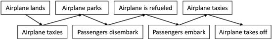
Figure 1.
A simplified illustration of a discrete event model, showing possible events taking place at an airport between the arrival and departure of an airplane.
4.2.2. Markov Models
Discrete Time Markov chains (DTMCs) are stochastic processes fulfilling the Markov property as explained by e.g., Kulkarni [79]. Stochastic processes consist of states and the probabilities to get from one state to another, called the transition probability. The Markov property assures that the next state of the chain only depends on the current state and the process is thus memoryless. DTMCs can be displayed as a state diagram for simple chains, displaying the different states the model can be in and the transition probabilities, an example is shown in Figure 2. A form that can be implemented and used in simulation software is the use of a transition matrix, including all the transition probabilities from each state to another, after sorting the states. DTMCs are already used in some of the existing models to model e.g., the significant wave height over time. A model combining DES with the DTMC state change mechanism is the most used modeling technique today. This provides simple state changes with transition probabilities and jumps from event to event, so times with no state changes do not have to be simulated. This again saves computational time and effort. The main problem with discrete models is that the turbine itself operates continuously. It experiences continuous loads from wind and wave that cause the failure events. In addition, the power output changes with the wind speed and is thus not constant between state changes. Depending on the wind speed and market price for electricity, the downtime losses are also continuous. Therefore, using a discrete model will always be a simplification of what is happening in reality. For use in the wind industry, discrete models can be a resource effective solution for modeling maintenance. However, they should be benchmarked with models that are more complex to provide confidence in the simplification.
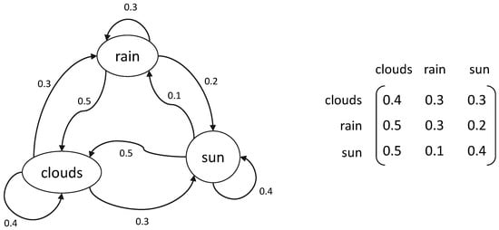
Figure 2.
An example of a Markov chain, displayed as both a state diagram (left) and a matrix with transition probabilities (right).
Continuous Time Markov Chains (CTMCs) are analogue to the DTMC, continuous stochastic processes fulfilling the Markov property. The main difference to the DTMCs is that instead of the transition probabilities, CTMCs use transition rates – the derivatives with respect to time of the transition probabilities between different states. While DTMCs can only model time steps of a fixed size, CTMCs offer the possibility to also describe phenomena that benefit from a continuous representation, such as the production, loads and weather. Additionally, CTMCs might be described with fewer parameters than DTMCs. While the implementation of a DTMC is very straight forward and much like a DES, CTMCs require more advanced methods. An example of a discrete Markov process is a random walk with an integer step-size, its scaling limit in dimension 1 (step-size converging to zero) is the continuous process called Wiener process, describing Brownian motion.
4.2.3. Differential Equations
Ordinary differential equations (ODEs) are equations, where the relationship between a variable t, an unknown function of this variable and the derivatives of this unknown function is known. Often, this independent variable t is time. This means that all variables in the function are dependent on time. When more than one unknown functions of the same variable exist, a system of ODEs can be used. Depending on the nature of the relationship , different mathematical approaches to finding a solution exist, providing exact solutions for integrable functions or numerical results using e.g., the Euler or Runge-Kutta method. Software that can be used for solving ODEs includes MATLAB and Maple.
In contrast to the ODEs, partial differential equations (PDEs) can have two or more independent variables. In addition to the time, this can be e.g., distance from a certain point. Examples for time-independent variables in wind farm maintenance modeling are the quality of repair or quality of a weather forecast. PDEs could be used for maintenance modeling; however, solving PDEs is not as straight forward as solving ODEs and the benefits most likely do not outweigh the complications in solving.
Stochastic differential equations (SDEs) are differential equations, where one or more terms are stochastic processes. The SDEs can be written in different forms. One of the most commonly used forms in physics are Langevin equations. These consist of ODEs using a deterministic function and an additional random term. The random term can take different forms, most commonly (Gaussian) white noise. Other forms of presenting SDEs include the Smoluchovski and Fokker-Planck equations, based on PDEs and the Itô equation, similar to the Langevin equation in differential notation. SDEs can be numerically solved by using e.g., the Euler-Maruyama method, the generalized Runge-Kutta method or Monte Carlo simulation. In the given problem setup of maintenance scheduling, SDEs can be a good way to incorporate the uncertainties in the variables. Existing models often use the mean for different input, such as the mean annual failure rate, mean times to repair or mean wind speed during downtime. With SDEs, these means can be used for the deterministic function and uncertainties in the observations can additionally be modeled by the random term. One of the drawbacks is the solving of the equations. Numerical methods to solve the equations are limited and often suffer from poor numerical convergence. Therefore, the main challenge when using SDEs for modeling the scheduling of maintenance will be to investigate the existence of solutions to the equations and the (numerical) calculation of these. Since the SDEs will depend largely on the input parameters, they cannot easily be used for different wind farm layouts and site, without changing the equation structure. This is another drawback, since a maintenance model should be able to capture the properties of different wind farms without the hassle of fitting a new set of equations to each case.
4.3. Conclusions about Modeling
A useful O&M model needs to be able to deal with several different input variables and potentially large data sets. Of the investigated candidates, all can capture the influencing factors in varying degrees of accuracy and with varying complexity. Those models that can use stochastic input are also able to provide stochastic distributions as output. For simple models, not capturing the uncertainties, DES and DTMCs can be combined to model the variations in the weather while still using discrete events as basis for the scheduling. This would, however, only cover uncertainties in the weather in a very basic way, e.g., through the probabilities of changes from one weather state to another in the Markov chain. Using continuous Markov models instead of discrete models provides the advantage of a better time-resolution, which can be beneficial to represent weather windows or repair durations. However, a validated discretization can capture the main properties. When researchers aim for more complexity and are not restricted by computational time, models that match the complexity of the input data are recommended. This means the most complex model that can be equipped with reliable data should be used. When no or only simple data sets are available, the complexity of the model should be adjusted accordingly. ODEs are a well-documented mathematical field. Once the model is described by ordinary differential equation, solving can be done by using one of many software options. However, since ODEs can only depend on one variable, this might be limiting in some cases. To avoid the dependence on one single variable, PDEs can be used. However, solving these is not as straight forward as solving ODEs. The most general way of modeling the scheduling of maintenance with differential equations are SDEs. These can also incorporate the uncertainties in the inputs, by including a random term. However, the existence and convergence of solutions is not guaranteed. Therefore, SDEs are not yet suitable for the use in the industry, before researchers have validated specific equations and investigated the necessary requirements for the existence of solutions.
4.4. Modeling in the Literature
As summarized in Table 4, many of the existing approaches use Monte Carlo simulations, combined with other modeling approaches. Many of the earlier models use DESs and Markov chain models. Other modeling approaches used are autogressive models and different kinds of stochastic processes.
Table 4.
This table summarizes the kinds of models presented in the literature.
5. Optimization
Optimization is the mathematical concept of finding the optimal solution to a (utility) function, given certain constraints to the solution. In the case of maintenance scheduling, the most obvious goal is to minimize the costs. Typical constraints are the availability of vessels, technicians and spare parts, environmental constraints, such as wave height and wind speeds and legal constraints, such as working hours, vessel speeds or limitations to routing. In mathematical optimization, one can distinguish between single- objective optimization and multi-objective optimization. The latter is the case when there is not one single goal for the optimization, but multiple. In the case of the offshore wind farm maintenance, this can mean to not only minimize costs, but at the same time maximize availability of the wind farm. This seems to be equivalent at the first glance, since downtime leads to production losses. However, maximizing availability will lead to a higher number of corrective maintenance actions that cannot be grouped together. This in turn influences the cost of maintenance. Legal restrictions and public opinion can be reasons for the wind farm operator to maximize availability, while still trying to minimize costs. In the following, we give an overview over different mathematical optimization algorithms and methods. The overview includes existing optimization techniques, with a focus on those that are implemented in the state-of-the-art maintenance models. For a detailed introduction to optimization, we want to refer to literature in the field, such as Diwekar [91]. Many introductory books on optimization focus on the type of problem (model) for which an optimal solution is found. We structure this section according to the type of optimization method.
5.1. Methods for Optimization
5.1.1. Algorithms
An algorithm can be figuratively described as a recipe that one can follow to reach an optimal solution to a given problem. The most famous example of optimization algorithms is most likely the Simplex algorithm, developed by George Dantzig. The Simplex algorithm was developed to be used in linear programming, but has since been extended to solve e.g., dual problems and network flow problems. A famous example from network optimization is the Kruskal algorithm, solving for a minimum spanning tree in an undirected graph. For unconstrained non-linear optimization problems, there exist the “steepest descent method” and Newton method for finding the optimum. For constrained non-linear problems, the Frank-Wolfe method, Penalty function method or Barrier function method can be applied. Integer programming models, such as the famous traveling salesman problem, can be solved by enumeration methods (only computational feasible for a small set of feasible solutions), relaxation and decomposition methods which are based on e.g., the Simplex method for linear programming. Additionally, branch and bound methods, originally developed by Land and Doig [92] can be applied. However, for integer programming models, heuristics are often used instead of algorithms, since they are less computational expensive and therefore time saving.
5.1.2. Heuristics
When using a heuristic method, as opposed to an algorithm, the convergence to the global optimum is not guaranteed. In general, those methods reach a solution faster and can also be used for more complex problems. One can distinguish between different types of heuristics. Constructive methods are methods in which the solution is constructed stepwise. For integer programming problems, one can start with free variables and fix a new variable in each step. Greedy algorithms are such an example of constructive heuristics. For the traveling salesman problem, heuristics such as the nearest neighbor algorithm or nearest addition algorithm have been shown to converge to the optimal solution. However, this does not hold in general. For vehicle routing problems, a heuristic such as presented by Clarke and Wright [93] can be used. However, it is not certain that it will produce a feasible solution. Local search heuristics improve the solution in each iteration by searching the neighborhood of the previous solution for a better one. Here it is possible to end up trapped in a local optimum. To improve the performance of such a local search heuristic, one can use different starting points to find several local optima. Then, the best one can be chosen as the global solution. Metaheuristics can aid in generating the starting point systematically. Examples for metaheuristics are the tabu search developed by Glover [94], where a memory is added to the local search. Simulated annealing, developed by Kirkpatrick et al. [95] generalizes the concept by choosing a random neighbor. Approximation algorithms, as presented in by Christofides [96] for the traveling salesman problem, can provide a bound for the optimal solution.
5.1.3. Stochastic Programming
Stochastic programming is not an optimization method, but rather a form of optimization problem. In stochastic programming, as opposed to deterministic programming, uncertainties can be incorporated in the analysis. One way to solve these kinds of problems is to use decision trees, where each possible event is modeling with its own branch, weighted with its probability of occurrence. Birge and Louveaux [97] present an introduction to the topic, including different solution methods and approximation methods. Stochastic programming can be relevant for offshore wind farm modeling, because of all the uncertainties involved in the planning of the maintenance tasks.
5.1.4. Dynamic Programming
Dynamic programming is also not a method itself, but rather a form of solving different optimization problems. We want to describe and discuss it here, because of its possible relevance to wind farm modeling. In dynamic programming, different stages in the optimization are modeled, where each stage can be interpreted as a time step. Dynamic programming allows to optimize both deterministic and stochastic programs. The two main fields of dynamic programming are “Markov decision processes”, modeling discrete states and decisions, and “control theory”, concerned with continuous states and decisions. For further reading about dynamic programming, we suggest Puterman [98] for Markov Decision Processes and Powell [99] for an emphasis on modeling and solving of larger problems. Since in an offshore wind farm the aim is to find the optimal solution over a long period of time (up to 25 years), it is beneficial to be able to update the inputs to the optimization over time, as more and more information about the system will be gathered. This can be achieved when using dynamic programming. As uncertainty should also be included, we believe tools from dynamic programming can be used to optimize the strategy for the maintenance of an offshore wind farm.
5.2. Conclusions about Optimization Methods
The discussion of the different optimization methods shows that for the case of optimizing the maintenance strategy of an offshore wind farm, different methods might be used. Stochastic programming shows the advantage of being able to represent the uncertainty in the inputs to the optimization. To solve these stochastic programs, the existing models use a Markov decision formulation with discrete time steps or discrete event steps. However, as discussed above, the existing models do only include uncertainties in very few of the influencing factors to the optimization. The present authors have shown the importance of including the uncertainty for additional parameters [100,101,102]. Therefore, we believe that approximate dynamic programming will be beneficial to solving the larger (stochastic) optimization problems, when the uncertainties are included for all influencing factors.
5.3. Optimization in the Literature
Most existing models provide multiple outputs, such as wind farm availability, production losses due to downtime, the number of failures, number of maintenance actions or costs of spare parts. However, an optimal strategy must be found in most cases by comparing the outputs for different strategies and manually selecting the best option. Some publications do present optimization methods. Sahnoun et al. [22] use a multi-criteria decision algorithm. Abdollahzadeh et al. [34] use multi-objective particle swarm optimization to determine the optimal reliability threshold for their preventive maintenance strategy. Pattison et al. [74] use for the optimization of the maintenance scheduling in their reliability centered maintenance model a multi-objective and multi-variable optimization. Hou et al. [103] use a particle swarm optimization—minimum spanning tree algorithm in their optimization of the cable layout in a given offshore wind farm.
6. Data Sources and Availability of Data
To fit and validate wind farm models, data for the input are needed. The closer the data is to the actual site conditions, the closer will a calculated optimum be to the actual optimal solution. Therefore, the availability of data directly influences how much decision support a model can provide. Unfortunately, not all types of data are easily available to public research. In the following we present data sources and which data different models are based on.
6.1. Data in the Literature
Feng et al. [4] provide data from nine different offshore wind farms in the UK, with the turbine manufacturer and type, rating, water depth, distance from shore as well as the operator. For production and turbine specific data, Sahnoun et al. [22] reference data from Kooijman et al. [51]. In their case study, Asgarpour and Sørensen [36] use the reference wind farm from the NORCOWE project. This is a reference wind farm located in the North Sea, 80km from the Danish coast. The reference wind farm consists of 80 DTU-10MW reference turbines and the water depth varies between 20 and 25 m. Another reference turbine is the one provided by Jonkman et al. [104]. This turbine has been used by, among others, Seyr and Muskulus [101].
6.1.1. Weather
Weather data is relatively easy to come by, as there are several meteorological measurement and re-analysis campaigns that provide data to the public. One of the data sources is the European Centre for Medium-Range Weather Forecasts (ECMWF) [105], who provide real-time and re-analysis data for, among others, ocean waves and wind speeds. The data sets vary in length and resolution, depending on the kind of data (ERA-interim re-analysis data for ocean waves is e.g., available from 1979, with a spatial resolution of 80 km). The three measurement campaigns FINO 1,2,3 from the “Bundesministerium für Wirtschaft und Energie” and “Projektträger Jülich” provided online from the Bundesamt für Seeschifffahrt und Hydrographie (BSH) [106] supply measurements of wave heights and wind speed in the offshore environment among their data. The records vary in lengths, with FINO 1 measuring data since 2003 and providing wind speed measurements in 10-min aggregated means. Feng et al. [4] provide monthly wind speed data for a UK offshore wind farm and annual average wind speed for four UK offshore wind farms. Climate data from an operating offshore wind farm NoordzeeWind is available for three years [107,108,109]. The WaveNet database from the Centre for Environment, Fisheries and Aquaculture Science (CEFAS) [110] provides real-time wave data from a network of buoys. The British Oceanographic Data Centre (BODC) [111] provide instrumentally recorded ocean current, tide, and wave data. Another source of weather data is the Norwegian Meteorological Institute [112], providing wind speed and direction as well as temperature and precipitation, with varying time-resolution dependent on the type and location of the measurement. Tolman [113] presented Wavewatch III, a wave model that can provide wave spectra at a selected location. Some publications use data from unpublished sources, such as from operating wind farms, airports, and an oil platform. Which weather data is used in which publication can be seen in Table 5.
Table 5.
This table summarizes which weather data has been used in the different models.
6.1.2. Failures
Data for failures are especially hard to find, since most manufacturers do not want to make their numbers public and because operators often do not have the complete failure history of their turbines. For onshore wind farms, failure data is easier to find than for offshore wind farms. The problem with using the failure rates of onshore turbines, when modeling offshore wind farms, is that offshore turbines often are of different types than onshore turbines and harsher weather conditions offshore lead to increased degradation and different failure causes than onshore. Data from onshore wind farms can be found in [114,115,116,117,118,119,120]. Tavner et al. [115] provide data from onshore wind farms on failure rate and sub-assembly reliability. They also provide a taxonomy for turbine sub-assemblies. A homogeneous Poisson process model is used to calculate the probability of failures from the MTBFs. They use data collected over 10 years in Germany and Denmark and assume that the failures are i.i.d. exponentially distributed. Sub-assembly failure rates and MTBF are provided for 12 sub-assemblies. Arabian-Hoseynabadi et al. [116] present a failure modes and effect analysis for onshore wind turbines. They present data from a real 2MW turbine (V80). 107 turbine parts, 16 failure modes and 25 root causes and present the top 10 for each category. Wilkinson et al. [117] provide a turbine taxonomy and reliability database listing fault events, failure rates, downtime, wind farm figuration and additional turbine information. They present the normalized failure rates for subsystems and assemblies of multiple manufacturers as well as the normalized hours lost due to the faults. Mean annual failure rates are available from Faulstich et al. [118] for different turbine subsystems. The annual failure rates and downtimes per failure have been calculated based on the data from 1500 wind turbines that were monitored between 1989 and 2006. Burton et al. [114] report the MTBFs for onshore turbines. Lin et al. [119] present common failures and failure frequencies as well as annual availability numbers for Chinese onshore wind farms. Reder et al. [120] in their paper give failure rates and downtimes for 4300 onshore turbines in the Mediterranean region.
Data from offshore wind farms is reported by [4,107,108,109,121,122]. Stiesdal and Madsen [121] provide a formula to calculate failure rates and present example failure rates, for offshore wind turbines. Data from Egmond aan Zee wind farm collected by NoordzeeWind has been reported for three consecutive years in [107,108,109]. Feng et al. [4] report operational performance such as availability and energy yield for four different UK offshore wind farms. Carroll et al. [122] present failure rates for 19 turbine components and four types of repairs/replacements. They also provide repair times, repair costs and number of technicians required for these same components and types. A summary of the different data sources and which data set is used in which model is presented in Table 6.
Table 6.
This table summarizes which failure data has been used in the different models. The data sources are Tavner [123], Wilkinson et al. [117], Faulstich et al. [118], Burton et al. [114], Stiesdal and Madsen [121], NoordzeeWind [107,108,109], Feng et al. [4] and Carroll et al. [122].
6.1.3. Costs
Also, data for costs of spare parts, technician salaries and vessel charter rates are not very easy to come by. The O&M costs for four UK offshore wind farms are reported in Feng et al. [4]. They also provide a comparison of the cost of energy for four different electricity generation technologies, namely coal gas, onshore wind, and offshore wind. Hofmann and Sperstad [16] do not present costs in their study, because they do not have any cost input data. Endrerud et al. [17] and Endrerud and Liyanage [21] use spare parts cost from Malcolm and Hansen [124]. Dalgic et al. [20] use vessel charter costs from Det Norske Veritas (DNV) [125] and Dalgic et al. [126]. They do not specify the source of the other cost data, but provide the numbers used in their case study. Ambühl et al. [63] mention the operational costs of a CTV from Besnard et al. [13] and assume that the transportation cost by helicopter is twice that of a vessel as suggested by van Bussel and Schöntag [127]. Shafiee et al. [23] present estimates for the annual OPEX in their life cycle cost analysis.
6.1.4. Vessel Information
Van Bussel and Bierbooms [46] present wind speed and wave height restrictions for five different access vessels. Out of these, one is fictitious and another one is based on optimistic assumptions. It is likely that the restrictions for vessels have been improved in the last 14 years. However, due to the lack of publicly available the values presented by Van Bussel and Bierbooms [46] are still widely used in research. Douard et al. [30] use wind speed and wave height limits. Feuchtwang and Infield [61] consider a threshold wave height for the access of 1.5m. Hofmann and Sperstad [16] do not provide any information about the access restrictions for the vessels. Sperstad et al. [19] present different methods of estimating the wave height restrictions for different vessel types. They show that using a single significant wave height limit has a similar outcome as using multiple access restrictions, but it depends on how this single value is estimated. Additionally, they also present some vessel data, such as capacity and size. Dalgic et al. [20] use information on the properties of different vessel types from O’Connor et al. [45], Tavner [123], Al-Salem et al. [128], Dai et al. [129] and Walker et al. [130]. Endrerud and Liyanage [21] present similar numbers as Sperstad et al. [19]. However, they do not say where they get these values from. Access restrictions reported by Sahnoun et al. [22] are 8 m/s wind speed and 1.5 m significant wave height. A source for these values is not provided. Ambühl et al. [63] use the access restrictions of 1.5 m significant wave height for boat access from Rademakers et al. [68] and wind speed of 20 m/s for helicopter access from Nielsen and Sørensen [10]. Rinaldi et al. [26] provide the maximum wave height and wind speed values for one existing vessel and one vessel under planning in their study.
7. Discussion
7.1. Factors to Consider
In the literature the factors influencing the planning and cost of maintenance are identified as (a) the component degradation and occurrence of failures, (b) availability of maintenance crew, spare parts and vessels, (c) transportation and vessel routing, (d) the weather, (e) economic parameters such as the electricity price, and (f) the maintenance strategy.
- (a)
- failure modeling, (i) different stochastic processes with failure rates are used by [11,12,14,16,17,19,20,21,22,26,30,32,33,34,37,39]; (ii) damage accumulation or time dependent failure rates are included in [10,17,21,22,26,30,31,32,35,36,37,38,40]
- (b)
- The availability of crew, parts and vessels is (i) considered as a (limited) resource, sometimes dependent on the failure type, by [12,13,16,17,20,21,22,25,26,31]; (ii) while [15,19] optimize in their analyses for the number of vessels.
- (c)
- Vessel routing and transportation has been studied by [10,25,41,46,52,53].
- (d)
- The weather is used as an input to the decision support models by [11,12,14,16,17,19,20,21,22,24,26,30,33,34,41,63,101];weather generation in the models is based on (i) Markov models by [12,16,19,30,56,57,59,62,64]; (ii) autoregressive by [11,14,20,66]; (iii) re-sampling by [31]; (iv) probability distributions by [33,34,61]; and (v) a Langevin process by [65].
- (e)
- For cost calculations (i) production losses due to downtime (indirect costs) are considered by [11,12,20,22,30,36]; (ii) maintenance costs in form of vessel hire, spare parts or worker salary (direct costs) are considered by [11,14,16,17,20,21,22,23,26,30,31,36,67].
- (f)
- The types of maintenance are discussed in the following Section 7.2.
7.2. Types of Maintenance
The different types of maintenance discussed in the review are (a) preventive maintenance, (b) condition monitoring, (c) condition-based maintenance and (d) corrective maintenance.
- (a)
- Preventive maintenance is conducted preventively on a fixed schedule to prevent failures from happening. It is included in the models and analyses by [16,17,20,21,22,26,32,36,46].
- (b)
- Condition monitoring can be used to monitor the performance of a wind turbine or component and can aid in predicting failures before they occur. Condition monitoring is studied by [63,67,70,71,72,73].
- (c)
- Condition-based maintenance is similar to preventive maintenance conducted to prevent failures. It is, however, based on the condition of the system instead of a fixed schedule. Condition-based maintenance is (i) considered in the models by [16,22,40]; and has been (ii) reviewed by [35,75].
- (d)
- Corrective maintenance must be carried out after a fault to return the component to a state in which it can perform its required function. Corrective maintenance is included in the models by [12,16,17,20,21,22,26,36].
7.3. Modeling
The existing decision support tools and models are based on DES, Markov models and autoregressive models. Alternatives to these models are other stochastic processes, or differential equations. Since solutions to differential equations are not always guaranteed, one needs to be careful with using these. For simulation-based models, DES and Markov models will therefore likely stay popular choices—also for offshore wind farm maintenance scheduling.
The existing models can capture most influencing factors; however, handling of uncertainty in the inputs is still an area that can be improved upon. Different wind farm layouts and locations can be included in the existing models, albeit being complex in implementation. The existing models lack an accessible way to handle uncertainties in the input and provide information about the variability in the output. Currently, mean values are reported and sensitivity analyses must be done by manually varying the inputs.
7.4. Optimization
Many different optimization tools exist, with stochastic and dynamic programming being able to include uncertainty and therefore potentially useful for decision support for wind farm maintenance planning. In the existing tools, no optimization is included and must be performed on a case basis by manually varying the input to compare different strategies. Optimization models have been presented by Abdollahzadeh et al. [34] to determine the reliability threshold for preventive maintenance, Pattison et al. [74] for maintenance scheduling decisions and Hou et al. [103] for optimal cable layout.
7.5. Data
The sources of data that have been referenced and used in the existing models are
- (a)
- for reference turbines: [51,104,131], and [132] for a reference wind farm;
- (b)
- for the weather: [105,106], NoordzeeWind [107,108,109], [110,111,112];
- (c)
- for failures: [114,116,117,119,120,123] for onshore data and [4,107,108,109,118,122] for offshore wind turbine failure data;
- (d)
- for cost information: [4,13,23,124,125,126];
- (e)
- for information about vessels: [10,22,26,41,45,46,68,123,128,129,130] seem to generally agree on a wave height limit of 1.5 m for boat access.
7.6. Usefulness of Models
The existing models used for decision support for offshore wind farm maintenance scheduling can be used by decision makers to gain more information before taking a decision. Most models can include different influential factors in the analysis. However, to optimize the maintenance strategy, the decision maker needs to manually vary the inputs to compare different strategies. None of the tools can provide a strategy-suggestion based on the inputs. The value of information for different input variables also must be calculated manually by conducting sensitivity studies and varying the inputs.
7.7. Trends and Future Work
Multiple authors mention collection of reliability data and improvement to reliability modeling as work needed in the future. It is mentioned that this can be achieved by including condition monitoring and condition-based maintenance in future models. As mentioned also by El-Thalji and Liyanage [7], there have been numerous academic contributions in the field of condition monitoring, diagnostics, and prognostics. Some possibilities for novel failure prediction methods are those presented by Artigao et al. [133], Gonzalez et al. [134], Tautz-Weinert and Watson [135]. Other sectors for improvement that have been mentioned are improved weather modeling—including more weather parameters, improved optimization methods and the treatment of uncertainty. The suggested method for future modeling is stochastic models.
8. Conclusions
In this review article, an overview over the current state of the art in operations and maintenance scheduling has been presented. The influential factors have been identified. Degradation and failure modeling; vessel, personnel, and spare part logistics; transportation and vessel routing; weather modeling; and cost estimation have been investigated in further detail. The types of maintenance have been presented and different maintenance strategies discussed. An overview over which maintenance strategies are included in which models has also been included. Modeling techniques and optimization methods have been presented and their use in current literature discussed. It was further discussed how the existing tools can aid with decision support. Finally, the importance and availability of necessary and useful data was discussed. The analysis and discussion have shown that existing models are not yet able to deal with uncertainties in all input factors. The weather input is well researched, also because of its relevance to fields other than offshore wind. Information about vessels and vessel routing is known and experience from other offshore industries can be used. In degradation and failure modeling, several approaches have been pursued; however, they show a dependence on data collection. Other factors, such as the duration of repairs, travel times, sensitivity of alarm systems or interaction between turbines or components are not as well integrated in state-of-the-art models. The mathematical techniques used at the moment are mostly simulation-based and optimization has to be done ‘by hand’. The discussion of methods has shown that concepts exist that are able to improve the modeling by using more complex methods to include uncertainty in the inputs or to avoid Monte Carlo simulation. Techniques to include an automated optimization have also been discussed which can increase the usefulness of models to decision support.
Author Contributions
M.M. proposed the idea of writing a review paper on the topic. H.S. and M.M. drafted the outline and structure of the paper. H.S. conducted the literature search and wrote the paper. M.M. reviewed the paper.
Funding
The work leading to this publication was financed by the AWESOME project (awesome-h2020.eu), which has received funding from the European Union’s Horizon 2020 research and innovation programme under the Marie Skłodowska-Curie grant agreement No 642108.
Acknowledgments
The authors thank three anonymous reviewers for their time and their comments, which helped improve the quality of the paper.
Conflicts of Interest
The authors declare no conflict of interest. The funders had no role in the design of the study; in the collection, analyses, or interpretation of data; in the writing of the manuscript, or in the decision to publish the results.
References
- World Wind Energy Association (WWEA). Half-Year Report 2014; World Wind Energy Association: Bonn, Germany, 2014. [Google Scholar]
- European Wind Energy Association (EWEA). Wind in Power 2015 European Statistics; Technical Report; World Wind Energy Association: Bonn, Germany, 2016. [Google Scholar]
- Wind Europe. The European Offshore Wind Industry—Key Trends and Statistics 2016; Technical Report; Wind Europe: Brussels, Belgium, 2017. [Google Scholar]
- Feng, Y.; Tavner, P.; Long, H. Early experiences with UK round 1 offshore wind farms. Proc. Inst. Civ. Eng. 2010, 163, 167–181. [Google Scholar] [CrossRef]
- Power, D.J. Decision Support Systems; Concepts and Resources for Managers; Reference and Research Book News; Book News, Inc.: Portland, OR, USA, 2002; Volume 17. [Google Scholar]
- Kessler, E.H. Encyclopedia of Management Theory; Sage Publications: Thousand Oaks, CA, USA, 2013. [Google Scholar]
- El-Thalji, I.; Liyanage, J.P. On the operation and maintenance practices of wind power asset: A status review and observations. J. Qual. Maint. Eng. 2012, 18, 232–266. [Google Scholar] [CrossRef]
- Hofmann, M. A review of decision support models for offshore wind farms with an emphasis on operation and maintenance strategies. Wind Eng. 2011, 35, 1–15. [Google Scholar] [CrossRef]
- Henderson, A.R.; Morgan, C.; Smith, B.; Sørensen, H.C.; Barthelmie, R.J.; Boesmans, B. Offshore wind energy in europe—A review of the state-of-the-art. Wind Energy 2003, 6, 35–52. [Google Scholar] [CrossRef]
- Nielsen, J.J.; Sørensen, J.D. On risk-based operation and maintenance of offshore wind turbine components. Reliab. Eng. Syst. Saf. 2011, 96, 218–229. [Google Scholar] [CrossRef]
- Dinwoodie, I.A.; McMillan, D.; Quail, F. Analysis of Offshore Wind Turbine Operation & Maintenance Using a Novel Time Domain Meteo-Ocean Modeling Approach; ASME Turbo Expo 2012; ASME: New York, NY, USA, 2012. [Google Scholar]
- Scheu, M.; Matha, D.; Hofmann, M.; Muskulus, M. Maintenance strategies for large offshore wind farms. Energy Procedia 2012, 24, 281–288. [Google Scholar] [CrossRef]
- Besnard, F.; Fischer, K.; Tjernberg, L.B. A model for the optimization of the maintenance support organization for offshore wind farms. IEEE Trans. Sustain. Energy 2013, 4, 443–450. [Google Scholar] [CrossRef]
- Dinwoodie, I.; McMillan, D.; Revie, M.; Lazakis, I.; Dalgic, Y. Development of a Combined Operational and Strategic Decision Support Model for Offshore Wind. Energy Procedia 2013, 35, 157–166. [Google Scholar] [CrossRef]
- Halvorsen-Weare, E.E.; Gundegjerde, C.; Halvorsen, I.B.; Hvattum, L.M.; Nonås, L.M. Vessel fleet analysis for maintenance operations at offshore wind farms. Energy Procedia 2013, 35, 167–176. [Google Scholar] [CrossRef]
- Hofmann, M.; Sperstad, I.B. NOWIcob—A tool for reducing the maintenance costs of offshore wind farms. Energy Procedia 2013, 35, 177–186. [Google Scholar] [CrossRef]
- Endrerud, O.E.V.; Liyanage, J.P.; Keseric, N. Marine logistics decision support for operation and maintenance of offshore wind parks with a multi method simulation model. In Proceedings of the 2014 Winter Simulation Conference, Savanah, GA, USA, 7–10 December 2014. [Google Scholar]
- Perveen, R.; Kishor, N.; Mohanty, S.R. Off-shore wind farm development: Present status and challenges. Renew. Sustain. Energy Rev. 2014, 29, 780–792. [Google Scholar] [CrossRef]
- Sperstad, I.B.; Halvorsen-Weare, E.E.; Hofmann, M.; Nonås, L.M.; Stålhane, M.; Wu, M. A Comparison of Single-and Multi-parameter Wave Criteria for Accessing Wind Turbines in Strategic Maintenance and Logistics Models for Offshore Wind Farms. Energy Procedia 2014, 53, 221–230. [Google Scholar] [CrossRef]
- Dalgic, Y.; Lazakis, I.; Dinwoodie, I.; McMillan, D.; Revie, M. Advanced logistics planning for offshore wind farm operation and maintenance activities. Ocean Eng. 2015, 101, 211–226. [Google Scholar] [CrossRef]
- Endrerud, O.E.V.; Liyanage, J.P. Decision Support for Operations and Maintenance of Offshore Wind Parks; Springer International Publishing: Cham, Switzerland, 2015. [Google Scholar]
- Sahnoun, M.; Baudry, D.; Mustafee, N.; Louis, A.; Smart, P.A.; Godsiff, P.; Mazari, B. Modelling and simulation of operation and maintenance strategy for offshore wind farms based on multi-agent system. J. Intell. Manuf. 2015, 1–17. [Google Scholar] [CrossRef]
- Shafiee, M.; Brennan, F.; Espinosa, I.A. A parametric whole life cost model for offshore wind farms. Int. J. Life Cycle Assess. 2016, 21, 961–975. [Google Scholar] [CrossRef]
- Gintautas, T.; Sørensen, J.D. Improved Methodology of Weather Window Prediction for Offshore Operations Based on Probabilities of Operation Failure. J. Mar. Sci. Eng. 2017, 5, 20. [Google Scholar] [CrossRef]
- Raknes, N.T.; deskaug, K.; Stålhane, M.; Hvattum, L.M. Scheduling of maintenance tasks and routing of a joint vessel fleet for multiple offshore wind farms. J. Mar. Sci. Eng. 2017, 5, 11. [Google Scholar] [CrossRef]
- Rinaldi, G.; Thies, P.; Walker, R.; Johanning, L. A decision support model to optimise the operation and maintenance strategies of an offshore renewable energy farm. Ocean Eng. 2017, 145, 250–262. [Google Scholar] [CrossRef]
- Nguyen, T.A.T.; Chou, S.Y. Maintenance strategy selection for improving cost-effectiveness of offshore wind systems. Energy Convers. Manag. 2018, 157, 86–95. [Google Scholar] [CrossRef]
- Eecen, P.; Braam, H.; Rademakers, L.; Obdam, T. Estimating costs of operations and maintenance of offshore wind farms. In Proceedings of the European Wind Energy Conference and Exhibition, Milan, Italy, 7–10 May 2007. [Google Scholar]
- Obdam, T.; Rademakers, L.; Braam, H.; Eecen, P. Estimating costs of operation & maintenance for offshore wind farms. In Proceedings of the European Offshore Wind Energy Conference, Berlin, Germany, 4–6 December 2007. [Google Scholar]
- Douard, F.; Domecq, C.; Lair, W. A probabilistic approach to introduce risk measurement indicators to an offshore wind project evaluation—Improvement to an existing tool ECUME. Energy Procedia 2012, 24, 255–262. [Google Scholar] [CrossRef]
- Asgarpour, M.; van de Pieterman, R. O&M Cost Reduction of Offshore Wind Farms: A Novel Case Study; ECN: Petten, The Netherlands, 2014. [Google Scholar]
- Shafiee, M.; Finkelstein, M. An optimal age-based group maintenance policy for multi-unit degrading systems. Reliab. Eng. Syst. Saf. 2015, 134, 230–238. [Google Scholar] [CrossRef]
- Joschko, P.; Widok, A.H.; Appel, S.; Greiner, S.; Albers, H.; Page, B. Modeling and simulation of offshore wind farm O&M processes. Environ. Impact Assess. Rev. 2015, 52, 31–39. [Google Scholar]
- Abdollahzadeh, H.; Atashgar, K.; Abbasi, M. Multi-objective opportunistic maintenance optimization of a wind farm considering limited number of maintenance groups. Renew. Energy 2016, 88, 247–261. [Google Scholar] [CrossRef]
- Alaswad, S.; Xiang, Y. A review on condition-based maintenance optimization models for stochastically deteriorating system. Reliab. Eng. Syst. Saf. 2017, 157, 54–63. [Google Scholar] [CrossRef]
- Asgarpour, M.; Sørensen, J.D. O&M modeling of offshore wind farms—State of the art and future developments. In Proceedings of the 2016 Annual Reliability and Maintainability Symposium (RAMS), Tucson, AZ, USA, 25–28 January 2016; pp. 1–6. [Google Scholar]
- Pliego Marugán, A.; García Márquez, F.P.; Pinar Pérez, J.M. Optimal maintenance management of offshore wind farms. Energies 2016, 9, 46. [Google Scholar] [CrossRef]
- Tibaldi, C.; Henriksen, L.C.; Hansen, M.H.; Bak, C. Wind turbine fatigue damage evaluation based on a linear model and a spectral method. Wind Energy 2016, 19, 1289–1306. [Google Scholar] [CrossRef]
- Scheu, M.N.; Kolios, A.; Fischer, T.; Brennan, F. Influence of statistical uncertainty of component reliability estimations on offshore wind farm availability. Reliab. Eng. Syst. Saf. 2017, 168, 28–39. [Google Scholar] [CrossRef]
- Welte, T.M.; Sperstad, I.B.; Sørum, E.H.; Kolstad, M.L. Integration of Degradation Processes in a Strategic Offshore Wind Farm O&M Simulation Model. Energies 2017, 10, 925. [Google Scholar]
- Stock-Williams, C.; Swamy, S.K. Automated daily maintenance planning for offshore wind farms. Renew. Energy 2018. [Google Scholar] [CrossRef]
- Wang, J.; Zhao, X.; Guo, X. Optimizing wind turbine’s maintenance policies under performance-based contract. Renew. Energy 2019, 135, 626–634. [Google Scholar] [CrossRef]
- Shafiee, M. Maintenance logistics organization for offshore wind energy: Current progress and future perspectives. Renew. Energy 2015, 77, 182–193. [Google Scholar] [CrossRef]
- Dinwoodie, I.; Endrerud, O.E.V.; Hofmann, M.; Martin, R.; Sperstad, I.B. Reference Cases for Verification of Operation and Maintenance Simulation Models for Offshore Wind Farms. Wind Eng. 2015, 39, 1–14. [Google Scholar] [CrossRef]
- O’Connor, M.; Lewis, T.; Dalton, G. Weather window analysis of Irish west coast wave data with relevance to operations & maintenance of marine renewables. Renew. Energy 2013, 52, 57–66. [Google Scholar]
- Van Bussel, G.; Bierbooms, W. The DOWEC Offshore Reference Windfarm: Analysis of Transportation for Operation and Maintenance. Wind Eng. 2003, 27, 381–391. [Google Scholar] [CrossRef]
- O’Connor, M.; Burke, D.; Curtin, T.; Lewis, T.; Dalton, G. Weather windows analysis incorporating wave height, wave period, wind speed and tidal current with relevance to deployment and maintenance of marine renewables. In Proceedings of the 4th International Congress on Ocean Energy, Dublin, Ireland, 17–19 October 2012. [Google Scholar]
- McMillan, D.; Ault, G.W. Quantification of condition monitoring benefit for offshore wind turbines. Wind Eng. 2007, 31, 267–285. [Google Scholar] [CrossRef]
- Wu, M. Numerical analysis of docking operation between service vessels and offshore wind turbines. Ocean Eng. 2014, 91, 379–388. [Google Scholar] [CrossRef]
- Ahn, D.; Shin, S.C.; Kim, S.Y.; Kharoufi, H.; Kim, H.C. Comparative evaluation of different offshore wind turbine installation vessels for Korean west–south wind farm. Int. J. Naval Archit. Ocean Eng. 2017, 9, 45–54. [Google Scholar] [CrossRef]
- Kooijman, H.; Lindenburg, C.; Winkelaar, D.; Van der Hooft, E. DOWEC 6 MW Pre-Design; Energy Research Center of the Netherlands (ECN): Petten, The Netherlands, 2003. [Google Scholar]
- Halvorsen-Weare, E.E.; Fagerholt, K.; Nonås, L.M.; Asbjørnslett, B.E. Optimal fleet composition and periodic routing of offshore supply vessels. Eur. J. Oper. Res. 2012, 223, 508–517. [Google Scholar] [CrossRef]
- Halvorsen-Weare, E.E.; Fagerholt, K. Optimization in offshore supply vessel planning. Optim. Eng. 2017, 18, 317–341. [Google Scholar] [CrossRef]
- Martini, M.; Guanche, R.; Losada, I.J.; Vidal, C. Accessibility assessment for operation and maintenance of offshore wind farms in the North Sea. Wind Energy 2017, 20, 637–656. [Google Scholar] [CrossRef]
- Schrotenboer, A.H.; uit het Broek, M.A.; Jargalsaikhan, B.; Roodbergen, K.J. Coordinating technician allocation and maintenance routing for offshore wind farms. Comput. Oper. Res. 2018, 98, 185–197. [Google Scholar] [CrossRef]
- Rothkopf, M.H.; McCarron, J.K.; Fromovitz, S. A weather model for simulating offshore construction alternatives. Manag. Sci. 1974, 20, 1345–1349. [Google Scholar] [CrossRef]
- Anastasiou, K.; Tsekos, C. Persistence statistics of marine environmental parameters from Markov theory, Part 1: Analysis in discrete time. Appl. Ocean Res. 1996, 18, 187–199. [Google Scholar] [CrossRef]
- Kuwashima, S.; Hogben, N. The estimation of wave height and wind speed persistence statistics from cumulative probability distributions. Coast. Eng. 1986, 9, 563–590. [Google Scholar] [CrossRef]
- Monbet, V.; Marteau, P.F. Continuous space discrete time Markov models for multivariate sea state parameter processes. In Proceedings of the Eleventh (2001) International Offshore and Polar Engineering Conference, Stavanger, Norway, 17–22 June 2001; International Society of Offshore and Polar Engineers: Mountain View, CA, USA, 2001. [Google Scholar]
- Lange, M. On the uncertainty of wind power predictions—Analysis of the forecast accuracy and statistical distribution of errors. J. Sol. Energy Eng. 2005, 127, 177–184. [Google Scholar] [CrossRef]
- Feuchtwang, J.; Infield, D. Offshore wind turbine maintenance access: A closed-form probabilistic method for calculating delays caused by sea-state. Wind Energy 2013, 16, 1049–1066. [Google Scholar] [CrossRef]
- Hagen, B.; Simonsen, I.; Hofmann, M.; Muskulus, M. A multivariate Markov weather model for O&M simulation of offshore wind parks. Energy Procedia 2013, 35, 137–147. [Google Scholar]
- Ambühl, S.; Kramer, M.; Sørensen, J.D. Risk-based Operation and Maintenance Approach for Wave Energy Converters Taking Weather Forecast Uncertainties into Account. In Proceedings of the Twenty-sixth (2016) International Ocean and Polar Engineering Conference, Rhodes, Greece, 26 June–2 July 2016; International Society of Offshore and Polar Engineers (ISOPE): Mountain View, CA, USA, 2016. [Google Scholar]
- Hersvik, K.; Endrerud, O.E.V. A high-fidelity weather time series generator using the Markov Chain process on a piecewise level. IOP Conf. Ser. 2017, 276, 012003. [Google Scholar] [CrossRef]
- Seyr, H.; Muskulus, M. Using a Langevin model for the simulation of environmental conditions in an offshore wind farm. J. Phys. Conf. Ser. 2018, 1104, 012023. [Google Scholar] [CrossRef]
- Taylor, J.W.; Jeon, J. Probabilistic forecasting of wave height for offshore wind turbine maintenance. Eur. J. Oper. Res. 2018, 267, 877–890. [Google Scholar] [CrossRef]
- Nilsson, J.; Bertling, L. Maintenance Management of Wind Power Systems Using Condition Monitoring Systems—Life Cycle Cost Analysis for Two Case Studies. IEEE Trans. Energy Convers. 2007, 22, 223–229. [Google Scholar] [CrossRef]
- Rademakers, L.; Braam, H.; Verbruggen, T. R&D needs for O&M of wind turbines. In Proceedings of the European Wind Energy Conference 2003, Madrid, Spain, 16–19 June 2003. [Google Scholar]
- Krokoszinski, H.J. Efficiency and effectiveness of wind farms—Keys to cost optimized operation and maintenance. Renew. Energy 2003, 28, 2165–2178. [Google Scholar] [CrossRef]
- Fu, Z.; Yuan, Y. Condition Health Monitoring of Offshore Wind Turbine based on Wireless Sensor Network. In Proceedings of the 2012 10th International Power & Energy Conference (IPEC), Ho Chi Minh City, Vietnam, 12–14 December 2012; pp. 649–654. [Google Scholar]
- Yang, W.; Tavner, P.J.; Crabtree, C.J.; Feng, Y.; Qiu, Y. Wind turbine condition monitoring: Technical and commercial challenges. Wind Energy 2014, 17, 673–693. [Google Scholar] [CrossRef]
- Bach-Andersen, M.; Rømer-Odgaard, B.; Winther, O. Flexible non-linear predictive models for large-scale wind turbine diagnostics. Wind Energy 2017, 20, 753–764. [Google Scholar] [CrossRef]
- Helsen, J.; Sitter, G.D.; Jordaens, P.J. Long-Term Monitoring of Wind Farms Using Big Data Approach. In Proceedings of the 2016 IEEE Second International Conference on Big Data Computing Service and Applications (BigDataService), Oxford, UK, 29 March–1 April 2016; pp. 265–268. [Google Scholar]
- Pattison, D.; Segovia Garcia, M.; Xie, W.; Quail, F.; Revie, M.; Whitfield, R.; Irvine, I. Intelligent integrated maintenance for wind power generation. Wind Energy 2016, 19, 547–562. [Google Scholar] [CrossRef]
- Leite, G.d.N.P.; Araújo, A.M.; Rosas, P.A.C. Prognostic techniques applied to maintenance of wind turbines: A concise and specific review. Renew. Sustain. Energy Rev. 2018, 81, 1917–1925. [Google Scholar] [CrossRef]
- Artigao, E.; Martín-Martínez, S.; Honrubia-Escribano, A.; Gómez-Lázaro, E. Wind turbine reliability: A comprehensive review towards effective condition monitoring development. Appl. Energy 2018, 228, 1569–1583. [Google Scholar] [CrossRef]
- European Committee for Standardization. CSN EN 13306:2010 Maintenance—Maintenance Terminology; European Committee for Standardization: Brussels, Belgium, 2010. [Google Scholar]
- Nance, R.E. A History of Discrete Event Simulation Programming Languages; ACM: New York, NY, USA, 1996. [Google Scholar]
- Kulkarni, V. Introduction to Modeling and Analysis of Stochastic Systems; Springer Texts in Statistics; Springer: New York, NY, USA, 2010. [Google Scholar]
- Pérez, E.; Ntaimo, L.; Byon, E.; Ding, Y. A stochastic DEVS wind turbine component model for wind farm simulation. In Proceedings of the 2010 Spring Simulation Multiconference, Orlando, FL, USA, 11–15 April 2010; p. 138. [Google Scholar]
- Byon, E.; Pérez, E.; Ding, Y.; Ntaimo, L. Simulation of wind farm operations and maintenance using discrete event system specification. SIMULATION 2011, 87, 1093–1117. [Google Scholar] [CrossRef]
- Pérez, E.; Ntaimo, L.; Ding, Y. Simulation of wind farm operations and maintenance. In Proceedings of the ASME Turbo Expo 2013: Turbine Technical Conference and Exposition, San Antonio, TX, USA, 3–7 June 2013. [Google Scholar]
- Leigh, J.M.; Dunnett, S.J. Use of Petri nets to model the maintenance of wind turbines. Qual. Reliab. Eng. Int. 2016, 32, 167–180. [Google Scholar] [CrossRef]
- Charniak, E. Bayesian networks without tears. AI Mag. 1991, 12, 50. [Google Scholar]
- Cryer, J.D.; Chan, K.S. Time Series Regression Models; Springer: Berlin, Germany, 2008; pp. 249–276. [Google Scholar]
- Murata, T. Petri nets: Properties, analysis and applications. Proc. IEEE 1989, 77, 541–580. [Google Scholar] [CrossRef]
- Staines, A.S. Rewriting Petri Nets as Directed Graphs. Int. J. Comput. 2011, 5, 289–297. [Google Scholar]
- Ko, R.K.; Lee, S.S.; Wah Lee, E. Business process management (BPM) standards: A survey. Bus. Process Manag. J. 2009, 15, 744–791. [Google Scholar] [CrossRef]
- Muehlen, M.z.; Recker, J. How Much Language Is Enough? Theoretical and Practical Use of the Business Process Modeling Notation. In Seminal Contributions to Information Systems Engineering: 25 Years of CAiSE; Bubenko, J., Krogstie, J., Pastor, O., Pernici, B., Rolland, C., Sølvberg, A., Eds.; Springer: Berlin/Heidelberg, Germany, 2013; pp. 429–443. [Google Scholar]
- Lee, J.H.; Kim, C.O. Multi-agent systems applications in manufacturing systems and supply chain management: A review paper. Int. J. Prod. Res. 2008, 46, 233–265. [Google Scholar] [CrossRef]
- Diwekar, U. Introduction to Applied Optimization; Springer Science & Business Media: Berlin, Germany, 2008; Volume 22. [Google Scholar]
- Land, A.H.; Doig, A.G. An Automatic Method of Solving Discrete Programming Problems. Econometrica 1960, 28, 497–520. [Google Scholar] [CrossRef]
- Clarke, G.; Wright, J.W. Scheduling of vehicles from a central depot to a number of delivery points. Oper. Res. 1964, 12, 568–581. [Google Scholar] [CrossRef]
- Glover, F. Future paths for integer programming and links to artificial intelligence. Comput. Oper. Res. 1986, 13, 533–549. [Google Scholar] [CrossRef]
- Kirkpatrick, S.; Gelatt, C.D.; Vecchi, M.P. Optimization by simulated annealing. Science 1983, 220, 671–680. [Google Scholar] [CrossRef] [PubMed]
- Christofides, N. Worst-Case Analysis of a New Heuristic for the Travelling Salesman Problem; Technical Report; Carnegie-Mellon Univ Pittsburgh Pa Management Sciences Research Group: Pittsburgh, PA, USA, 1976. [Google Scholar]
- Birge, J.R.; Louveaux, F. Introduction to Stochastic Programming; Springer Series in Operations Research and Financial Engineering; Springer: Berlin, Germany, 2011. [Google Scholar]
- Puterman, M.L. Markov Decision Processes: Discrete Stochastic Dynamic Programming; John Wiley & Sons: Hoboken, NJ, USA, 2005. [Google Scholar]
- Powell, W.B. Approximate Dynamic Programming: Solving the Curses of Dimensionality; Wiley Series in Probability and Statistics; John Wiley & Sons: Hoboken, NJ, USA, 2011. [Google Scholar]
- Seyr, H.; Muskulus, M. Interaction of repair time distributions with a weather model. In Proceedings of the 29th International Congress on Condition Monitoring and Diagnostics Engineering Management (COMADEM 2016), Xi’an, China, 20–22 August 2016. [Google Scholar]
- Seyr, H.; Muskulus, M. Value of information of repair times for offshore wind farm maintenance planning. J. Phys. Conf. Ser. 2016, 753, 092009. [Google Scholar] [CrossRef]
- Seyr, H.; Muskulus, M. How Does Accuracy of Weather Forecasts Influence the Maintenance Cost in Offshore Wind Farms? In Proceedings of the 27th International Ocean and Polar Engineering Conference, San Francisco, CA, USA, 25–30 June 2017; International Society of Offshore and Polar Engineers: Mountain View, CA, USA, 2017. [Google Scholar]
- Hou, P.; Hu, W.; Chen, C.; Chen, Z. Overall Optimization for Offshore Wind Farm Electrical System. Wind Energy 2017, 20, 1017–1032. [Google Scholar] [CrossRef]
- Jonkman, J.; Butterfield, S.; Musial, W.; Scott, G. Definition of a 5-MW Reference Wind Turbine for Offshore System Development; National Renewable Energy Laboratory: Golden, CO, USA, 2009.
- European Centre for Medium-Range Weather Forecasts (ECMWF). Public Datasets. Available online: https://www.ecmwf.int (accessed on 11 December 2018).
- Bundesamt für Seeschifffahrt und Hydrographie (BSH). FINO Datenbank. Available online: http://fino.bsh.de/ (accessed on 11 December 2018).
- NoordzeeWind. Wind Farm Egmond aan Zee Operations Report 2007; NoordzeeWind: Egmond aan Zee, The Netherlands, 2008. [Google Scholar]
- NoordzeeWind. Wind Farm Egmond aan Zee Operations Report 2008; NoordzeeWind: Egmond aan Zee, The Netherlands, 2009. [Google Scholar]
- NoordzeeWind. Wind Farm Egmond aan Zee Operations Report 2009; NoordzeeWind: Egmond aan Zee, The Netherlands, 2010. [Google Scholar]
- Centre for Environment, Fisheries and Aquaculture Science (CEFAS). CEFAS—WaveNet. Available online: www.cefas.co.uk/cefas-data-hub/wavenet/ (accessed on 11 December 2018).
- British Oceanographic Data Centre (BODC). BODC–Marine Data Available to Download. Available online: https://www.bodc.ac.uk/ (accessed on 11 December 2018).
- Norwegian Meteorological Institute. eKlima Free Access to Weather- and Climate Data from Norwegian Meteorological Institute from Historical Data to Real Time Observations. Available online: eKlima.met.no (accessed on 11 December 2018).
- Tolman, H. Validation of WAVEWATCH III Version 1.15 for a Global Domain; Technical Report, NOAA/NWS/NCEP/OMB Tech. Note 213; U.S. Department of Commerce, National Oceanic and Atmospheric Administration, National Weather Service, National Centers for Environmental Prediction: Washington, DC, USA, 2002.
- Burton, T.; Jenkins, N.; Sharpe, D.; Bossanyi, E. Wind Energy Handbook; John Wiley & Sonss: Hoboken, NJ, USA, 2011. [Google Scholar]
- Tavner, P.; Xiang, J.; Spinato, F. Reliability analysis for wind turbines. Wind Energy 2007, 10, 1–18. [Google Scholar] [CrossRef]
- Arabian-Hoseynabadi, H.; Oraee, H.; Tavner, P. Failure modes and effects analysis (FMEA) for wind turbines. Int. J. Electr. Power Energy Syst. 2010, 32, 817–824. [Google Scholar] [CrossRef]
- Wilkinson, M.; Hendriks, B.; Spinato, F.; Gomez, E.; Bulacio, H.; Roca, J.; Tavner, P.; Feng, Y.; Long, H. Methodology and results of the ReliaWind reliability field study. In Proceedings of the European Wind Energy Conference and Exhibition 2010, EWEC 2010, Warsaw, Poland, 20–23 April 2010; Volume 3, pp. 1984–2004. [Google Scholar]
- Faulstich, S.; Hahn, B.; Tavner, P.J. Wind Turbine downtime and its importance for offshore deployment. Wind Energy 2011, 14, 327–337. [Google Scholar] [CrossRef]
- Lin, Y.; Tu, L.; Liu, H.; Li, W. Fault analysis of wind turbines in China. Renew. Sustain. Energy Rev. 2016, 55, 482–490. [Google Scholar] [CrossRef]
- Reder, M.; Gonzalez, E.; Melero, J.J. Wind turbine failures—Tackling current problems in failure data analysis. J. Phys. Conf. Ser. 2016, 753, 072027. [Google Scholar] [CrossRef]
- Stiesdal, H.; Madsen, P.H. Design for reliability. In Proceedings of the Copenhagen Offshore Wind International Conference, Copenhagen, Denmark, 26–28 October 2005. [Google Scholar]
- Carroll, J.; McDonald, A.; McMillan, D. Failure rate, repair time and unscheduled O&M cost analysis of offshore wind turbines. Wind Energy 2016, 19, 1107–1119. [Google Scholar]
- Tavner, P. Offshore Wind Turbines: Reliability, Availability and Maintenance; Institution of Engineering and Technology: London, UK, 2012. [Google Scholar]
- Malcolm, D.J.; Hansen, A.C. WindPACT Turbine Rotor Design Study: June 2000–June 2002 (Revised); Technical Report; National Renewable Energy Lab. (NREL): Golden, CO, USA, 2006.
- Det Norske Veritas (DNV). DNV-OS-H101. Marine operations, general. In DNV Offshore Standards (OS) H; DNV: Oslo, Norway, 2011; Volume 101. [Google Scholar]
- Dalgic, Y.; Dinwoodie, I.A.; Lazakis, I.; McMillan, D.; Revie, M. Optimum CTV Fleet Selection for Offshore Wind Farm O&M Activities. In Proceedings of the European Safety and Reliability Conference ESREL 2014, Wroclaw, Poland, 14–18 September 2014. [Google Scholar]
- Van Bussel, G.; Schöntag, C. Operation and maintenance aspects of large offshore windfarms. In Proceedings of the European Wind Energy Conference, Dublin Castle, Ireland, October 1997; Bookshop for Scientific Publications: Slane County Meath, Republic of Ireland, 1997; pp. 272–275. [Google Scholar]
- Al-Salem, K.; Al-Nassar, W.; Tayfun, A. Risk analysis for capsizing of small vessels. Ocean Eng. 2006, 33, 788–797. [Google Scholar] [CrossRef]
- Dai, L.; Ehlers, S.; Rausand, M.; Utne, I.B. Risk of collision between service vessels and offshore wind turbines. Reliab. Eng. Syst. Saf. 2013, 109, 18–31. [Google Scholar] [CrossRef]
- Walker, R.T.; van Nieuwkoop-McCall, J.; Johanning, L.; Parkinson, R.J. Calculating weather windows: Application to transit, installation and the implications on deployment success. Ocean Eng. 2013, 68, 88–101. [Google Scholar] [CrossRef]
- Bak, C.; Zahle, F.; Bitsche, R.; Kim, T.; Yde, A.; Henriksen, L.C.; Hansen, M.H.; Blasques, J.P.A.A.; Gaunaa, M.; Natarajan, A. The DTU 10-MW Reference Wind Turbine; Danish Wind Power Research: Fredericia, Denmark, 2013. [Google Scholar]
- Bak, T.; Graham, A.; Sapronova, A.; Chen, Z.; Knudsen, T.; Sørensen, J.D.; Florian, M.; Hou, P.; Asgarpour, M. Norcowe reference wind farm. Annual Report Norcowe 2014; Norcowe: Bergen, Norway, 2015; pp. 38–40. [Google Scholar]
- Artigao, E.; Honrubia-Escribano, A.; Gomez-Lazaro, E. Condition monitoring of a wind turbine doubly-fed induction generator through current signature analysis. J. Phys. Conf. Ser. 2017, 926, 012008. [Google Scholar] [CrossRef]
- Gonzalez, E.; Stephen, B.; Infield, D.; Melero, J.J. On the use of high-frequency SCADA data for improved wind turbine performance monitoring. J. Phys. Conf. Ser. 2017, 926, 012009. [Google Scholar] [CrossRef]
- Tautz-Weinert, J.; Watson, S. Condition monitoring of wind turbine drive trains by normal behaviour modelling of temperatures. In Proceedings of the Conference for Wind Power Drives 2017: Tagungsband zur Konferenz, BoD–Books on Demand, Aachen, Germany, 7–8 March 2017; Volume 3, p. 359. [Google Scholar]
© 2019 by the authors. Licensee MDPI, Basel, Switzerland. This article is an open access article distributed under the terms and conditions of the Creative Commons Attribution (CC BY) license (http://creativecommons.org/licenses/by/4.0/).