Simultaneous Optimisation of Cable Connection Schemes and Capacity for Offshore Wind Farms via a Modified Bat Algorithm

Abstract

Offshore wind energy has attracted worldwide attention and investments in the last decade due to the stability and abundance of wind resources. As one of the main components of this, internal array cables have a great impact on the levelised cost of energy of offshore wind farms, and thus their connection layout is a matter of concern. In this paper, a classical mathematical problem—the traveling salesman problem, which belongs to the field of graph theory—is applied to solve the offshore wind farm cable connection layout optimization problem. Both the capital investment on cables, cable laying, and the cost of power losses associated with array cables are considered in the proposed model. A modified bat algorithm is presented to resolve the problem. Furthermore, a cable crossing detection method is also adopted to avoid obtaining crossed cable connection layouts. The effectiveness was verified through a case study.

1. Introduction

As one of the most environmentally friendly renewable energies, the wind is an ideal resource for meeting the greatly increasing electricity demand while reducing the impacts on the environment [1]. According to the statistics of the European Wind Energy Association, 15.6% of total power capacity was from wind energy in 2015, which has a 13.2% increased share of the market compared to the data in 2000 [2]. Offshore wind energy has unique advantages [3] such as higher energy density, stable wind distribution as well as reduced impacts on residents. Consequently, the penetration of offshore wind energy is expected to continuously increase [4]. However, the huge investment an offshore wind farm represents makes the economic operation infeasible without subsidies at an earlier time. Therefore technological innovation and development to lower the levelised cost of energy (LCoE) of the wind farm are attracting attention globally.

As introduced in [5], up to 30% of the capital expenditure (CAPEX) of the offshore wind farm is related to its electrical system, of which the internal array cables and their associated costs make up a large proportion. As a result, a good deal of research has been conducted on the optimization of the cable connection layout to make a cost-effective wind farm. When bigger cables are applied to transmit the energy, the overall energy losses will be reduced, which contributes to a large amount of revenue increase within the wind farm’s operating lifetime. However, more CAPEX is paid out. Hence, in the offshore wind farm cable connection layout problem (OWFCCLP), the cable connection layout, as well as the sectional area of each cable, should be optimized simultaneously considering the cable’s current carrying capacity [6]. As mentioned in [7], the OWFCCLP is a highly non-convex combinatory optimization problem where the combination of the electrical equipment is required to be optimized under the power system constraints. Deterministic algorithms may fail to resolve this kind of problem [8]. In comparison, the heuristic algorithm can find a sub-optimal solution in an acceptable time. Hence, this has been widely used in solving OWFCCLP [8,9,10,11,12,13,14,15]. Different sea cable connection layouts—the string structure, ring structure, and multiloop structure—on a three-dimensional seabed were analyzed in [8], wherein a multiple loop cable connection structure was proposed and the overall length of cables was minimized by the particle swarm optimization algorithm (PSO). In [9], the common electrical system schemes of the offshore wind farm and electrical component costs are analyzed. Based on that, the optimization model for OWFCCLP was proposed and solved by a genetic algorithm (GA). The above works only considered one type of cable and thus could only minimize the length of cables in each branch instead of minimizing the overall cost. To further reduce the cost, a mixed integer linear programming method was proposed in [10] which considered the cable section area’s impact on the cable connection scheme. The authors in [11] proposed an adaptive particle swarm optimization minimum spanning tree method to solve the OWFCCLP using cables with different sectional areas. In [12], in addition to different sectional areas, the collection system and transmission system were both considered in the OWFCCLP. It encoded the topology to a binary string and solved the problem via standard GA. However, the power losses are not taken into account in [10,11,12]. In [13], the power losses were considered in the optimization model, and the proposed model was solved by a hybrid immune GA algorithm. Similarly, a dynamic minimum spanning tree algorithm was proposed in [14] to solve the OWFCCLP, which considered the power loss. Besides this, considering both the power losses and cable sectional area selection, the open multiple travelling salesman problem (OMTSP) was compared with OWFCCLP in [15]; based on their common properties, a new optimization model was established and solved by GA. However, the thinnest cable which satisfies the cable’s current carrying capacity was selected as the optimized cable, and thus the impact of the power losses on the layout formulation was actually not taken into account.

In the OWFCCLP, a crossed cable connection layout is not desired. Firstly, it will increase the installation cost [16]; secondly, it incurs thermal perturbation, which decreases the cable’s current carrying capacity. In addition, crossed cables are easily damaged which, endangers the safe operation of the entire offshore wind farm. Considering the huge costs maintenance [17], a method was proposed in [17] to solve the OWFCCLP while ensuring an uncrossed cable connection layout using mathematical programming. However, the impact of power loss on the layout formulation is taken into account. Despite the power loss cost (PLC) being considered in the objective function in [13,14,15], its impact on the cable sectional area was not modeled in [13,14], while reference [15] neglects the influence of PLC on the cable selection by using cables with the same sectional area. In addition, the uncrossed cable connection layout was studied in [17], whereas the PLC’s influence was neglected. Through the literature study, it can be seen that the power loss impacts on the cable sectional area selection and cable connection layout formulation were not well studied. It would be beneficial if the impact of the power losses and the cable crossing to the cable connection layout formulation are considered at the same time, thus delivering a better offshore wind farm electrical system design. Thus, an OWFCCLP model was proposed in this paper. Compared to the above works, the PLC’s impact on the cable connection layout formulation as well as the cable sectional area selection were both considered in the optimization model, and an uncrossed cable connection layout was ensured during the layout formulation process. The internal array cable and its laying costs are considered as the CAPEX while the revenue losses due to power losses are regarded as the operational cost (OPEX). To solve the problem, an updated bat algorithm (BA) is adopted, and the proposed model is validated via a case study.

The paper is organized as follows: Section 2 describes the OWFCCLP which is derived based on the open multiple traveling salesman problem. Section 3 provides the modified bat algorithm to solve the problem. An irregularly shaped wind farm is chosen as the study case to demonstrate the proposed method in Section 4. Section 5 draws conclusions and proposes further work.

2. Mathematical Models

The mathematical model of the total cost is expressed for OWFCCLP at first. Then, the open multiple travelling salesman problem (OMTSP) for OWFCCLP is introduced. Finally, the OMTSP model-based OWFCCLP is specified.

2.1. OWFCCLP

The wind turbines (WTs) are widely spread in the open sea area. In order to collect the power generated from each WT economically, the cable connection layout should be optimized to make the electrical system cost effective. Since the power losses along the cables reduce the energy reached at the point of common coupling and thus influence the revenue for the wind farm owner, this part of revenue loss should be counted in the cable connection layout and cable type selection optimization process which formulates the OWFCCLP.

In this paper, the objective function is set up by considering both the CAPEX and OPEX. The CAPEX of the offshore wind farm includes the cable cost and the cable trenching cost, while the costs of the energy losses in the internal network are considered as the OPEX. The overall target is to minimize the total cost to ensure the best return on investment for investors during the entire operational lifetime of the wind farm. The mathematical model of the total cost can be expressed as

$$C_{Total}{=\min (Z}_{Trench}{+Z}_{Cable}{+Z}_{EnergyLoss}),$$

(1)

where Z_Trench means the total trenching cost of the internal array cables, Z_Cable is the investment on cables and Z_EnergyLoss represents the cost of energy losses associated with the array cables in the internal network during the entire lifetime of the wind farm. The detailed expressions of each cost variable can be seen in the following:

$$Z_{Trench}{=C}_{Trench}\cdot ({\displaystyle \sum _{k=1}^K\sum _{m=1}^M\sum _{p=1}^N}{L}_m{g}_{G_T,k,m,p}+{\displaystyle \sum _{k=1}^K\sum _{m=1}^M\sum _{\begin{array}{c}{m}^{\prime }=1,\\ m^{\prime }\ne m\end{array}}^M\sum _{p=1}^N}{L}_{{m,m}^{\prime }}^{\prime }{g}_{G_T{,k,m,m}^{\prime },p}^{\prime }),$$

(2)

It can be seen in Equation (2) that Z_Trench is related to the total length of cables. Similarly, it can be calculated according to the cable connection layout and the cable size for each path, which can be written as follows:

$$Z_{Cable}=3({\displaystyle \sum _{k=1}^K\sum _{m=1}^M\sum _{p=1}^N}{C}_p{L}_m{g}_{G_T,k,m,p}+{\displaystyle \sum _{k=1}^K\sum _{m=1}^M\sum _{\begin{array}{c}{m}^{\prime }=1,\\ m^{\prime }\ne m\end{array}}^M\sum _{p=1}^N}{C}_p{L}_{{m,m}^{\prime }}^{\prime }{g}_{G_T{,k,m,m}^{\prime },p}^{\prime }),$$

(3)

The power losses of the cables are related to the resistance and are proportional to the square of the passed current. The expression of power losses is expressed as

$$Z_{EnergyLoss,Unit}{=(I}_{rated}{)}^2\cdot ({\displaystyle \sum _{k=1}^K\sum _{m=1}^M\sum _{p=1}^N}{{(O}_{G_T,k,m,p})}^2{L}_m{R}_p{g}_{G_T,k,m,p}+{\displaystyle \sum _{k=1}^K\sum _{m=1}^M\sum _{\begin{array}{c}{m}^{\prime }=1,\\ m^{\prime }\ne m\end{array}}^M\sum _{p=1}^N}{{(O}_{G_T{,k,m,m}^{\prime },p}^{\prime })}^2{L}_{{m,m}^{\prime }}^{\prime }{R}_p{g}_{G_T{,k,m,m}^{\prime },p}^{\prime }),$$

(4)

where I_reated is the rated current of the WT:

$$I_{rated}=\frac{P_{rated}}{\sqrt{3}\cos \mu U_{rated}},$$

(5)

Furthermore, considering the duration time of the peak energy loss and interest rate of each year, Z_Energyloss can be written as

$$Z_{EnergyLoss}=3{\displaystyle \sum _{\tau =1}^T}{(1+D)}^{\tau }{\tau }_{\Delta }{C}_{EnergyLoss}{Z}_{EnergyLoss,Unit},$$

(6)

It should be noticed that, for the protection of the electrical equipment, the maximum current flowing in each cable is capped by an upper limit, which means the number of WTs carried by a specified cable is limited. A feasible cable connection layout must strictly meet the maximum load flow constraint; in other words, the actual current going through each cable should be no more than I_max,p, which formulates a new constraint as follows:

$$\begin{array}{c}{I}_{rated}{(O}_{G_T,k,m,p}{g}_{G_T,k,m,p}+{\displaystyle \sum _{\begin{array}{c}{m}^{\prime }=1,\\ m^{\prime }\ne m\end{array}}^M}{O}_{G_T{,k,m,m}^{\prime },p}^{\prime }{g}_{G_T{,k,m,m}^{\prime },p}^{\prime })\le I_{max,p},\\ \forall k=1,2,\cdots ,K,\forall m=1,2,\cdots ,M, \forall m=1,2,\cdots ,M, \forall p=1,2,\cdots ,N,\end{array}$$

(7)

where I_max,p is determined according to the size of the cable which corresponds to its ability to prevent overload. Cables with various sectional areas have different current carrying capacities; the specifications of the cables used in this paper are included in

Table A1. Basic technical and economic data for 18/30 KV, XRUHAKXS cable [18].

Type No.	Sectional Area	Price [Euro/km]	Resistance [Ω/km]	Ampacity [A]
T1	50	6466.701	0.588	175
T2	70	8113.770	0.42	210
T3	95	8447.516	0.31	250
T4	120	10,593.922	0.245	285
T5	150	10,957.479	0.196	320
T6	185	11,875.338	0.159	360
T7	240	13,719.673	0.123	420
T8	300	17,798.218	0.098	475
T9	400	21,240.014	0.074	540
T10	500	25,053.752	0.059	605
T11	630	34,709.087	0.047	675
T12	800	41,960.429	0.037	750

[18].

2.2. OMTSP Model for OWFCCLP

OMTSP can be defined as follows: K traveling salesmen must visit M cities from a predetermined departure city, and a suitable travel path should be defined to meet the scheduled goal (such as the shortest path or minimum cost) under certain constraints. The constraints of OMTSP include the following:

Constraint 1: Each traveling salesman must start from the same departure city before visiting other cities, whereas each one does not have to return to the departure city;

Constraint 2: Each city (except the departure city) can be visited only once by one traveling salesman;

Constraint 3: Each traveling salesman should maintain continuity during the visits; that is, the traveling salesman cannot visit two cities at the same time after visiting one city (except the departure city).

Comparing the definition of OMTSP with OWFCCLP, it can be seen that the departure city, visited cities, and access path of a traveling salesman in the OMTSP can be analogized as the offshore substation (OS), WTs and the cable connection scheme of feeder lines in the OWFCCLP. The OMTSP is completely consistent with the definition of OWFCCLP. However, OWFCCLP only meets constraint 1 and constraint 2 of the OMTSP while constraint 3 is violated. Hence, a further constraint is added into the OWFCCLP to meet constraint 3 of the OMTSP; that is, only two cables are allowed to be connected to one WT (one entering and one leaving cable) in each feeder line. The constraint can be expressed as:

$$\begin{array}{c}{g}_{G_T,k,m,p}+{\displaystyle \sum _{m^{\prime }=1}^M}{g}_{G_T,k, m^{\prime },m,p}^{\prime }={\displaystyle \sum _{m^{\prime }=1}^M}{g}_{G_T,k,m, m^{\prime },p}^{\prime }+g_{G_T,k,m,p}^{″},\\ \forall k=1, 2, \cdots , K,\forall m=1, \cdots , M\end{array}$$

(8)

2.3. Assumptions

In this simulation, some assumptions are made as follows.

(1)

The number and positions of the OS and WTs are given;

(2)

All cables are assumed to be 3-core cross-linked polyethylene (XLPE) AC cables;

(3)

The cable length is selected according to the geometrical distance without considering detailed practical situations, such as the barriers, restriction in the sea, and the length from the WT foundation to the sea bottom;

(4)

The cost of cable laying and purchasing is linearly proportional to the cable length;

(5)

The power factor is assumed to be 0.75;

(6)

All WTs are assumed to be operated at 1 p. u. voltage.

Combining with the assumptions above, the OMTSP model is modified and thus well suitable for solving the OWFCCLP. To help get an optimized solution, a BA algorithm is adopted in this paper, which is introduced in the next section.

3. Optimization Method

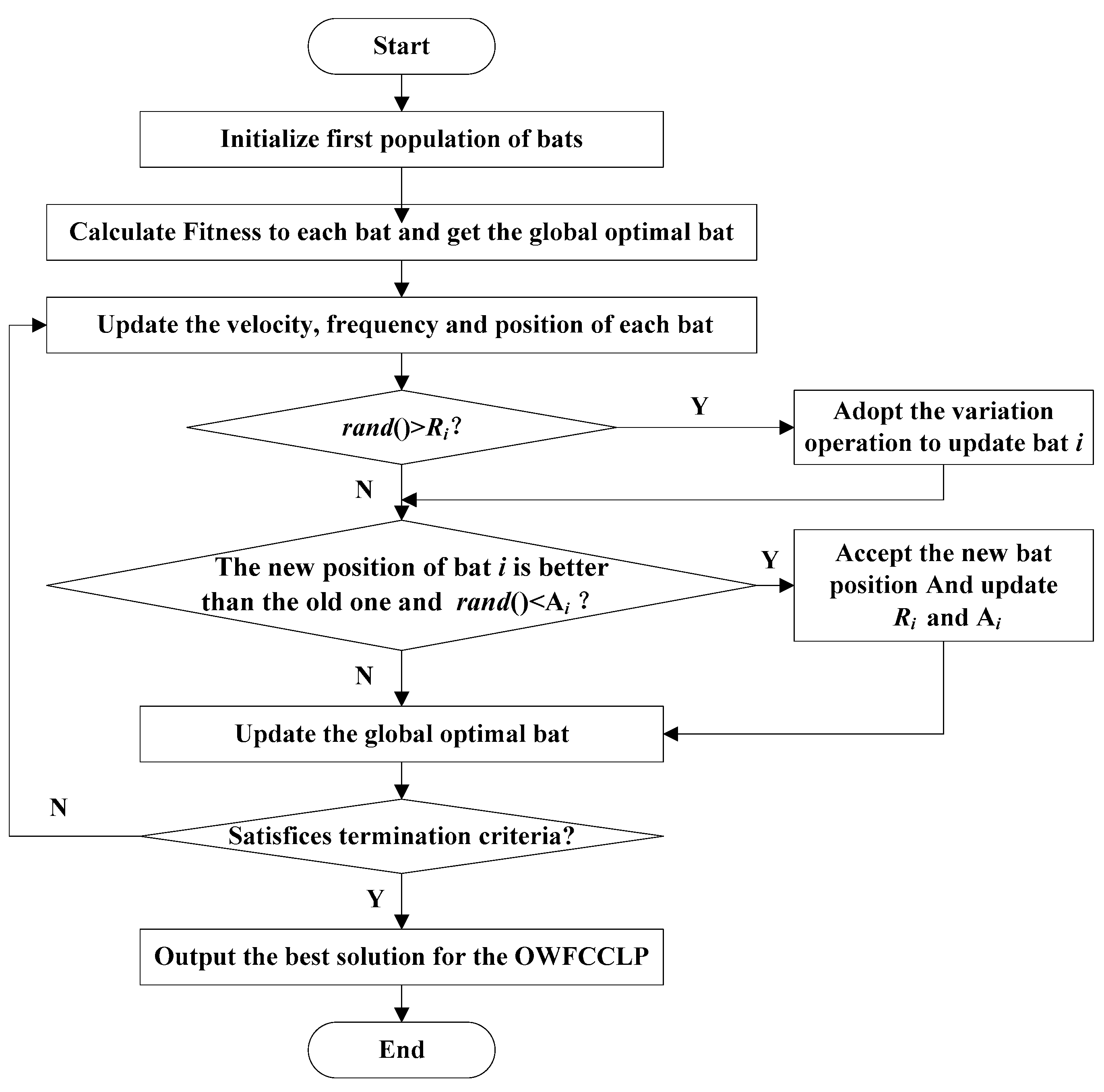
The principle of BA is introduced at first; then, the encoding and decoding process which are the two critical steps of solving the optimization problem by BA are specified. Furthermore, the cable crossing detection algorithm is proposed to determine if there are cable crossings in the final solution. The fitness function used to evaluate the results after each iteration is presented at last.

3.1. Bat Algorithm

BA is a heuristic algorithm proposed by Yang in 2010 and is inspired by the echolocation behavior of micro-bats [19]. BA simulates bats’ preying process via echolocation in the natural world. According to the distance between the prey and bats, they adjust the ultrasonic wavelength and the frequency of the firing pulse, capturing their prey eventually. The earlier studies have shown that BA can solve constrained and unconstrained optimization problems with superior efficiency and robustness [20,21]. Although BA was proposed recently, there are many variants of BA that have been successfully applied to different fields and problems, such as the traveling salesman problem [22,23], vehicle routing problem [24,25], 0–1 knapsack problem [26,27], and unmanned aerial vehicle path planning problem [28]. Hence, the BA is applied in this work. The iterative update of BA consists of the position of bats, velocity, frequency update operation, mutation update operation, the bat loudness and emission frequency update. In one of our previous works [29], a modified BA was proposed which can be expressed as

$$\begin{array}{cc}{f}_{i,t+1}=\{\begin{array}{l}{f}_{i,t}+(f_{\mathrm{rand}}-f_{i,t})/\theta ,f_{\mathrm{rand}}>f_{i,t}\\ f_{i,t}, f_{\mathrm{rand}}\le f_{i,t}\end{array}& \begin{array}{c}\begin{array}{cc}{f}_{i,t}\in [0,1],& f_{\mathrm{rand}}\in [0,1]\end{array}\\ \theta >1\end{array}\end{array}$$

(9)

$$v_{i,t+1}=v_{i,t}+(x_{i,t}-x_{\ast ,t})\times f_{i,t}$$

(10)

$$x_{i,t+1}=x_{i,t}+v_{i,t+1}$$

(11)

Assuming $x_{i,t}=\left[x_{i,t,1}, x_{i,t,2}, \cdots , x_{i,t,w}\right]$ has w dimensions, the corresponding velocity $v_{i,t}=\left[v_{i,t,1}, v_{i,t,2}, \cdots ,v_{i,t,w}\right]$. $x_{i,t,j}$ and $v_{i,t,j}$ are both positive integers and $x_{i,t,j}\in \left[1,w\right]$, $v_{i,t,j}\in [1,w]$, $j=1, 2, \cdots ,w$. From (9) to (11), it can be seen that the bat’s position is updated by the velocity and frequency so that a better position can be found iteratively. In order to improve the searching capacity of bats, a variation operation is introduced which can be expressed mathematically as follows:

$$x_{i,t+1}=\mathrm{Vary}(x_{i,t})$$

(12)

The specified procedure of (12) is that of inserting one position, $x_{i,t}$, into another position. Then, other positions will make the corresponding movement. By doing so, the diversity of bats is increased, which is helpful for increasing the possibility of finding a global optimal solution. To trigger the variation operation and facilitate the position updating process, the pulse loudness, $A_{i,t+1}$, and emission frequency, $R_{i,t+1}$, are designed in BA, which work as two pointers. The mathematical expressions are expressed in the following:

$$A_{i,t+1}=\alpha A_{i,t}, A_{i,0}\in [0,1], 0<\alpha <1$$

(13)

$$R_{i,t+1}=R_{i,0}\times \left[1-\exp (-\gamma t)\right], R_{i,0}\in [0,1], \gamma >0$$

(14)

where $R_{i,0}$ is the initial emission frequency of bat i. The main responsibilities of $A_{i,t+1}$ and $R_{i,t+1}$ are to balance the global searching ability and the local searching ability of BA. The flow chart of BA is shown in Figure 1.

As can be seen in Figure 1, there are mainly 8 steps in the BA, which are specified in the following:

Step 1: Initialization of the first population of bats (the population size is Q), including the position, velocity, frequency, loudness, and pulse emission rate of bat i;

Step 2: Calculate the fitness of each bat and obtain the global optimal bat position;

Step 3: Update the velocity, frequency, and position of each bat;

Step 4: If rand() > R_i, the variation operation will be adopted to update bat i;

Step 5: If the new position of bat i is better than the old one and rand() > R_i, then the new position becomes the new current position of bat i, and the loudness and pulse emission rate of bat i are updated by updated operations of loudness and pulse emission rate;

Step 6: Update the global optimal position of bats;

Step 7: If the termination criterion is not reached, then go to Step 3;

Step 8: Output the best solution of the OWFCCLP.

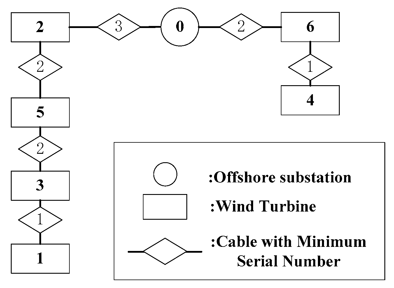
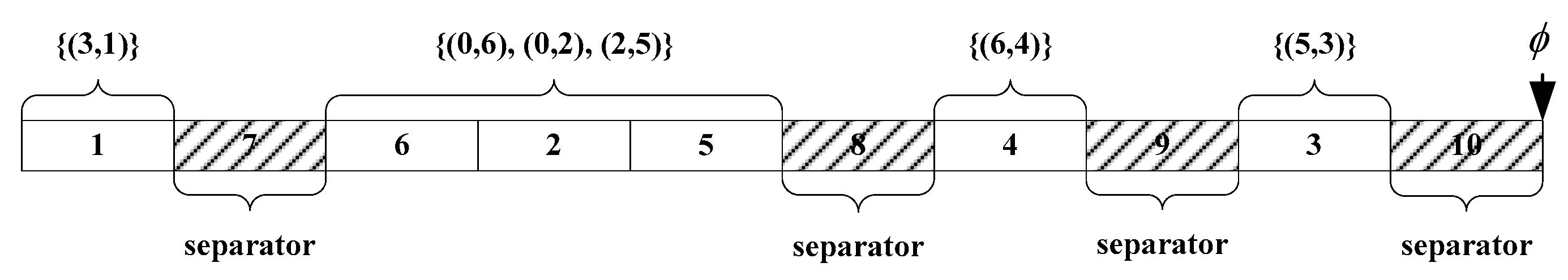
3.2. Encoding and Decoding

The encoding and decoding scheme is the first and most important step to solving the optimization problem [30]. In this paper, the bat position, $x_{i,t}=[x_{LevelOne,i,t},x_{LevelTwo,i,t}]$, contains both the information of the cable connection layout of the wind farm ($x_{LevelOne,i,t}$ ⋲ [1,2,…,W]) and the available cable sectional areas ($x_{LevelTwo,i,t}⋲\left[1,2,\dots ,H\right]$), where W is equal to M + K-1 and H equal to M + N-2 respectively.

To illustrate the encoding process, an example is shown below. In this example, it is assumed that there are 6 WTs in total which can be connected by a maximum of 4 feeder lines. There are 5 different types of cables in store and W = 9, H = 10. Assuming the first generation of bat positions,$x_{1,1}=[x_{LevelOne,1,1},x_{LevelTwo,1,1}];$ then, the encoding of bats could be $x_{LevelOne,1,1}$ = [2,5,3,1,7,6,4,8,9], $x_{LevelTwo,1,1}$ = [1,7,6,2,5,8,4,9,3,10]. Then, the decoding process of the example is shown in the following:

a. In $x_{LevelOne,1,1}$, 1 to 6 represent the sequence number of WTs while 7 to 9 show the separators, which are illustrated in Figure 2.

In Figure 2, $x_{LevelOne,1,1}$ is divided into 4 sections by the separators, which shows that 6 WTs are unevenly arranged into each feeder line. WT $\left[2,5,3,1\right]$ belong to feeder line one while WT $\left[6,4\right]$, $\phi$, and $\phi$ belong to feeder line 2 to 4, respectively. $\phi$ means the null set: in other words, we do not need feeder line 3 and 4 in this design.

In this work, zero indicates the OS. One possible cable connection layout—(0,2), (2,5), (5,3), (3,1), (0,6), and (6,4)—is shown in Figure 3.

According to the cable’s current carrying limitation, the thinnest cable sectional area (type) will be selected in the first layer. As shown in Figure 3, the selected cable types are 3, 2, 2, 1, 2, and 1, respectively, in this example. Therefore, the cable connection layout based on the minimum cable type selection criterion is decided.

b. Decoding $x_{LevelTwo,1,1}$ based on the $x_{LevelOne,1,1}$. In $x_{LevelTwo,1,1}$, 1 to 6 represent the output cables connected to WT 1 to 6 while 7 to 10 represent the separators, as shown in Figure 4.

As can be seen in Figure 4, $x_{LevelTwo,1,1}$ was divided into 5 sections by the separators. The number of the separator is decided according to the available number of cable types. By doing so, the 6 WTs were divided into 5 groups: that is, $\{(3,1)\}$, $\{(0,6), (0,2), (2,5)\}$, $\{(6,4)\}$, $\{(5,3)\}$, and $\phi$. The cables in the same group will be updated by the randomly generated number in this layer, which is called the cable type incremental number (CTIN) in this work. In order to update the cable type for each branch, the numbers in this layer represent the increased value compared to the cable type selected in the first layer. For instance, if the previous cable type is 1 and the number in this layer is 4, then the final selected cable type is 5.

In Figure 5, it can be seen that the cable connection layout is the same as in Figure 3. However, the cable type of branch (3,1), (0,2), (5,3), (6,4), (2,5), and (0,6) has been changed from 1, 3, 2, 1, 2, 2 into 1, 4, 5, 3, 3, 3.

Besides this, the practical feeder line used in the cable connection layout is usually limited by the substation transformer. It is assumed that the maximum number of feeder lines is no more than K. In this case, as long as K is big enough, there is no need to specify the number of feeder lines, and BA can converge and obtain a better cable connection layout. This is more beneficial for the free convergence of the algorithm and in getting a more reasonable cable connection layout.

3.3. Cable Crossing Detection

To reduce the OPEX and failure rate, the crossed cable connection layout is not desirable in the OWFCCLP. Hence, a specific algorithm [16] is introduced in this work to prevent the emergence of crossed cables.

It is assumed that there are crossed cables in a certain cable connection layout which is shown in Figure 6.

In Figure 6, the coordinates of 4 WTs are shown as $E_1=({ex}_1,{ey}_1)$, $E_2=({ex}_2,{ey}_2)$, $E_3=({ex}_3,{ey}_3), \mathrm{and} E_4=({ex}_4,{ey}_4)$. If segment E₁E₂ crosses E₃E₄, then there $a\in \left[0,1\right]$ and $b\in \left[0,1\right]$ should exist, which satisfy Equation (15) as follows:

$$\{\begin{array}{l}a\cdot e{x}_1+(1-a)\cdot e{x}_2=b\cdot e{x}_3+(1-b)\cdot e{x}_4\\ a\cdot e{y}_1+(1-a)\cdot e{y}_2=b\cdot e{y}_3+(1-b)\cdot e{y}_4\end{array}$$

(15)

Furthermore, the matrix reformulation of Equation (15) can be obtained as follows:

$$\left[\begin{array}{cc}e{x}_1-e{x}_2& e{x}_4-e{x}_3\\ e{y}_1-e{y}_2& e{y}_4-e{y}_3\end{array}\right]\left[\begin{array}{c}a\\ b\end{array}\right]=\left[\begin{array}{c}e{x}_4-e{x}_2\\ e{y}_4-e{y}_2\end{array}\right]$$

(16)

By substituting the following equations into Equation (16),

$$EM=\left[\begin{array}{cc}e{x}_1-e{x}_2& e{x}_4-e{x}_3\\ e{y}_1-e{y}_2& e{y}_4-e{y}_3\end{array}\right]=\left[\begin{array}{cc}e{m}_{11}& e{m}_{12}\\ e{m}_{21}& e{m}_{22}\end{array}\right], EQ=\left[\begin{array}{c}e{x}_4-e{x}_2\\ e{y}_4-e{y}_2\end{array}\right]=\left[\begin{array}{c}e{q}_1\\ e{q}_2\end{array}\right], EZ=\left[\begin{array}{c}a\\ b\end{array}\right],$$

Equation (15) can then be rewritten as

$$EZ={(EM)}^{-1}EQ=\frac{1}{\det (EM)}\left[\begin{array}{c}e{m}_{22}\cdot e{q}_1-e{m}_{12}\cdot e{q}_2\\ -e{m}_{21}\cdot e{q}_1+e{m}_{11}\cdot e{q}_2\end{array}\right]$$

(17)

From (17), the values of both a and b can be easily calculated; then, the judgment of crossed cables can be fulfilled by detecting the value of a and b. By searching all the connection layouts ergodically, the total number of crossed cables, CI, can then be obtained.

3.4. Fitness

In order to cultivate a better generation during the evolutionary process of BA, the population must be evaluated by the fitness function. In order to prevent the crossed cable connection layout, the fitness function is revised to consider the impact of the crossed cables on the objective function using the penalty factor. Then, the fitness function can be expressed as follows:

$$Fit=C_{Total}+NP\times CI$$

(18)

where PN is the penalty factor, which is set as 1e6 in this work. The smaller the $Fit$ is, the better the cable connection layout will be. It can also be noticed that the crossed cables will increase the fitness function significantly, and they will, therefore, be eliminated in the bat position updating process.

4. Case Study

In this paper, an offshore wind farm with an irregular layout is selected as the study case. The reference wind farm layout is introduced at first. Then, the results obtained by the proposed method are presented and analyzed. The experimental simulation environment is Windows 10 OS, Intel Corei7-6800K [email protected], 16 GB RAM. The program is compiled using the C++ language, and the simulation software is Visual Studio 2010.

4.1. Reference Wind Farm

In this work, an offshore wind farm, which is composed of 50 Enercon E82-2.0 MW WTs is selected as the studied case. The WT coordinates are listed in

Table A2. Wind farm coordinates [31].

No.	X	Y	No.	X	Y	No.	X	Y
0	−845,561.14	5,061,423.55	17	−838,944.09	5,066,377.42	34	−837,311.59	5,064,423.56
1	−846,551.67	5,060,657.03	18	−838,601.34	5,066,593.06	35	−837,046.43	5,064,944.85
2	−845,954.33	5,060,883.50	19	−838,254.91	5,067,022.42	36	−836,945.46	5,065,693.19
3	−845,527.75	5,061,275.42	20	−838,120.77	5,065,964.24	37	−836,358.59	5,064,898.32
4	−845,598.66	5,061,754.17	21	−837,641.43	5,066,676.94	38	−836,352.80	5,065,308.05
5	−845,165.18	5061991.33	22	−837,581.87	5,067,741.13	39	−836,241.70	5,065,869.39
6	−844,046.87	5,062,169.24	23	−837,280.64	5,068,024.39	40	−836,589.68	5,066,437.29
7	−843,544.15	5,062,635.89	24	−836,815.44	5,068,294.17	41	−836,676.07	5,066,772.53
8	−843,199.17	5,063,651.03	25	−836,651.02	5,068,694.55	42	−835,622.32	5,065,795.89
9	−842,515.33	5,063,926.61	26	−836,241.70	5,068,813.00	43	−835652.71	5,066,202.24
10	−842,472.25	5,064,270.21	27	−835,946.15	5,069,149.66	44	−838,182.00	5,062,211.31
11	−842,115.03	5,064,891.65	28	−835,783.29	5,069,459.35	45	−837,952.90	5,061,721.73
12	−841,235.38	5,064,495.28	29	−835,408.92	5,069,717.16	46	−837,510.41	5,061,924.97
13	−840,852.89	5,064,706.43	30	−834,981.67	5,069,791.29	47	−836,793.51	5,061,876.67
14	−840,610.21	5,065,009.31	31	−838,299.11	5,064,348.29	48	−835,788.52	5,061,431.10
15	−840,407.83	5,065,378.29	32	−838,180.11	5,064,832.08	49	−836,051.90	5,061,783.80
16	−839,244.99	5,066,102.06	33	−837,878.54	5,065,140.60	50	−835,673.52	5,061,985.40

[31] while the technical and economic information of the wind farm is shown in

Table A3. Other basic technical and economic data of the wind farm [18].

Item	Value	Item	Value
$P_{rated}$	2.0 MW	$D$	0.02
$U_{rated}$	30.0 kV	${\tau }_{\Delta }$	1700 h
$T$	10 Year	$C_{Trench}$	18,632 Euro/km
$cos \mu$	0.75	$C_{EnergyLoss}$	42.283 Euro/MWh

[18]. It is worthy of note that there are usually limited types of cables that are available in the actual wind farm construction process. Hence, two scenarios are presented in this work to show the effectiveness of the proposed method in both an ideal situation and relatively realistic case.

4.2. Simulation Results and Discussion

In each scenario, three models are compared. The first model (BA_MIN) forms the cable connection layout scheme according to the minimum cross-sectional cable selection rule, which means the thinnest cable that satisfies the cable current constraint will be selected. The second model (BA_FREE) considers the impact of the cable sectional area selection on the objective function. The last model (MBA) is designed based on the BA_FREE while taking the impacts of crossed cables on the final layout into account. To compare their performances, all the algorithms are run with the same termination criterion: that is, terminated at 800 s. The input parameters of BA are identical for each model: that is Q = 400, θ = 150, α = 0.999, γ = 0.001. Each algorithm is run 10 times independently, and the best results are selected as the global optimal solution. In order to illustrate the selected cable sectional area, different colors are adopted in the following figures. The simulation results of each scenario are included in

Table 1. Simulation results. PLC: power loss cost.

Description	Units	Scenario I			Scenario II
		MBA	BA_FREE	BA_MIN	MBA	BA_FREE	BA_MIN
Trenching cost of cables	[kEUR]	1126.94	1091.77	1063.08	1128.29	1136.05	1130.98
Purchase cost of cables	[kEUR]	2625.46	2883.08	2645.9	2803.31	2790.14	2664.48
PLC	[kEUR]	2161.84	1928.86	2333.12	2009.57	1977.65	2136.07
Total cost	[kEUR]	5914.24	5903.72	6042.09	5941.17	5903.84	5931.53

.

4.2.1. Scenario I: Ideal Case

In this scenario, it is assumed that 12 sorts of cables in total can be used. The optimized layouts are shown in Figure 7.

In Figure 7, the red stars indicate the positions of WTs while the green square shows the OS.

It can be seen that thicker cables are adopted if the MBA and BA_FREE methods are used, which agrees with the fact that MBA_MIN merely used the thinnest cables that satisfy the current constraint. It can also be seen that the cable connection layouts found by BA_FREE and BA_MIN are with crossed cables, while no crossed cables exist in the layout found by MBA, as illustrated in Figure 7a. The statistic results for running each model using BA are shown in Figure 8.

In Figure 8, the pink diamond, blue cross, and red star represent the results obtained by BA_MIN, BA_FREE, and MBA, respectively. It can be seen that the layouts found by MBA and BA_FREE are always better than the layouts found by BA_MIN in 10 trails. The fitness value corresponds to the CPU time of the best trial for each method, as shown in Figure 9.

It can be seen in Figure 9 that BA_MIN converged earliest among the three models, which stabilized after 150 s, while MBA and BA_FREE stabilized at 300 s and 680 s, respectively. Though this situation varies in each trail, the algorithm can stabilize after 750 s even in the worst case. In the following scenario, the available cable types are reduced to approximate the real case.

4.2.2. Scenario II: 5 Sorts of Cables

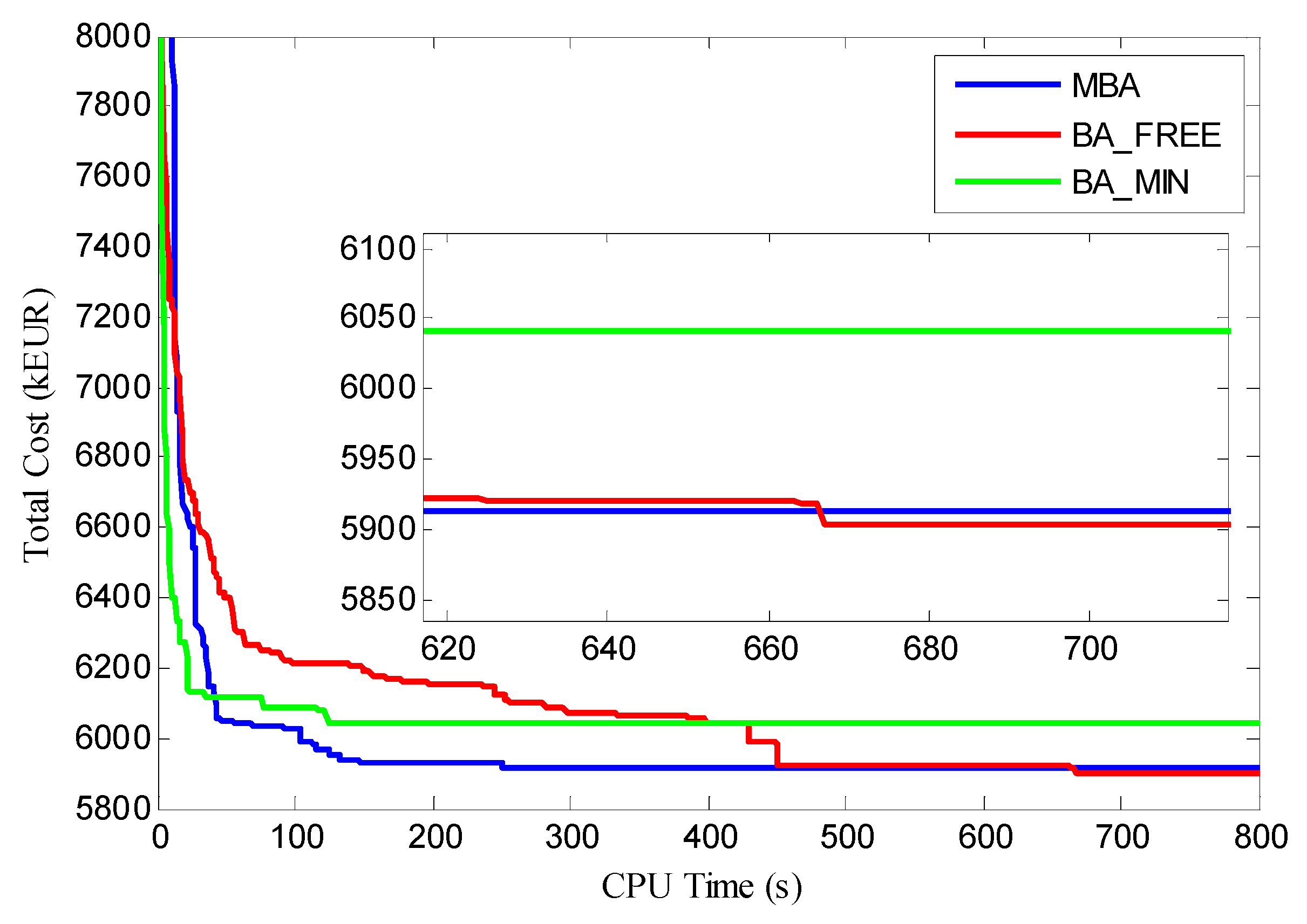
In reality, due to the reducing cost of volume production, the commonly used cables may have a lower single price. Hence, even a cable with a thicker sectional area, if commonly used, may be cheaper than one with a thinner sectional area. That is why the cable connection layout optimization work is usually done based on limited types of cables. In this section, it is assumed that 5 sorts of cables with different sectional areas are at hand. The optimized layouts with such a cable database are shown in Figure 10.

Similar to Scenario I, the layouts obtained by MBA and BA_FREE adopted the thickest cables (T11 cable) as can be seen in Figure 10a,b, while thinner cables illustrated with yellow lines can be found in (c). Similarly, the layout found by the MBA has no crossed cables while the BA_FREE and BA_MIN are opposite. The 10 trials are shown in Figure 11.

In Figure 11, it can be seen that the optimal solution found by the MBA, BA_FREE, and BA_MIN appeared in the fourth, eighth and second trial. Within the three models, the optimal solution is found by the BA_FREE. The fitness value corresponds to the CPU time of the best trail for each method is drawn in Figure 12.

As can be seen in Figure 12, the MBA converged earliest in this scenario, which stabilized at 250 s, while BA_FREE and BA_MIN stabilized at 440 s and 400 s, respectively. All the methods can stabilize after 500 s even in the worst case in this scenario.

4.2.3. Discussion

To compare the performance of the optimized layouts, the detailed information of each scenario using MBA, BA_FREE or BA_MIN is listed in Table 1. The detailed information of the cable connection scheme of each scenario is given in

Table A4. The connections for optimized layouts obtained by different algorithms in scenario I.

Cable Types	Connections for the Optimized Layout by MBA	Connections for the Optimized Layout by BA_FREE	Connections for the Optimized Layout by BA_MIN
12	--	--	--
11	(0,5)	--	--
10	(5,11)	(0,18), (0,6),	(0,15), (0,6), (0,12),
9	(0,6), (6,7), (0,8), (8,9), (11,19), (19,22),	(0,7), (7,31), (18,19), (19,22), (6,11), (11,15),	(15,19), (6,31), (12,13),
8	--	(31,32),	(19,22), (31,32), (13,14),
7	(0,31), (7,12), (12,13), (9,10), (10,14), (22,23), (23,24), (0,44)	(32,33), (33,34), (5,8), (8,9), (22,23), (23,24), (24,25), (0,44), (44,45), (45,46), (15,16), (16,17), (17,20),	(22,23), (32,33), (14,16),
6	(31,34), (13,32), (14,15), (24,25), (44,45)	(34,35), (35,37), (0,5), (26,27), (46,47), (20,21), (21,41),	(23,24), (33,34), (0,44), (16,17),
5	(34,35), (32,33), (15,16), (25,26), (45,46)	(37,38), (25,26), (41,40),	(24,25), (0,5), (34,35), (44,45), (17,18)
4	--	--	(25,26), (5,7), (35,37), (45,46), (18,20)
3	(35,37), (33,36), (16,17), (26,27), (46,47)	(38,42), (0,2), (9,10), (10,12), (12,13), (27,28), (28,29), (47,49), (49,48), (40,39)	--
2	(37,38), (36,39), (17,18), (0,3), (27,28), (47,49)	(0,3)	(26,27), (7,8), (37,38), (46,47), (20,21)
1	(38,42), (42,43), (39,40), (40,41), (18,20), (20,21), (3,2), (2,1), (0,4), (28,29), (29,30), (49,50), (50,48)	(42,43), (2,1), (13,14), (29,30), (48,50), (0,4), (39,36)	(27,28), (28,29), (29,30), (8,9), (9,10), (10,11), (0,4), (0,3), (3,2), (2,1), (38,39), (39,42), (42,43), (47,49), (49,50), (50,48), (21,41), (41,40), (40,36)

and

Table A5. The connections for optimized layouts obtained by different algorithms in scenario II.

Cable Types	The Connections for the Optimized Layout by MBA	The Connections for the Optimized Layout by BA_FREE	The Connections for the Optimized Layout by BA_MIN
11	(0,5)	(0,5)	--
9	(0,6), (0,7), (7,12), (5,11), (11,22), (0,8)	(5,8), (8,10), (0,9), (9,22), (0,7), (7,12)	(0,19), (19,22), (0,6), (0,8), (8,10), (0,5), (5,9)
7	(6,31), (31,32), (32,33), (33,34), (12,13), (13,20), (20,21), (21,41), (0,44), (44,45), (45,46), (22,23), (23,24), (24,25), (25,26), (8,9), (9,10), (10,14), (14,15)	(10,11), (11,16), (16,17), (17,18), (22,23), (23,24), (24,25), (25,26), (0,44), (44,45), (45,46), (0,6), (6,31), (31,32), (32,33), (12,13), (13,14), (14,15), (15,20)	(22,23), (23,24), (0,44), (6,7), (7,31), (10,11), (11,15), (9,12), (12,13)
5	(34,35), (41,40), (46,47), (26,27), (15,16)	(18,19), (26,27), (46,47), (33,34), (20,36)	(24,25), (25,26), (44,45), (45,46), (31,32), (32,33), (15,16), (16,17), (13,14), (14,20)
3	(35,37), (37,38), (38,36), (0,3), (3,2), (2,1), (40,39), (39,42), (42,43), (47,49), (49,50), (50,48), (0,4), (27,28), (28,29), (29,30), (16,17), (17,18), (18,19)	(19,21), (21,41), (41,40), (0,4), (27,28), (28,29), (29,30), (47,49), (49,50), (50,48), (34,35), (35,37), (37,38), (0,3), (3,2), (2,1), (36,39), (39,42), (42,43)	(26,27), (27,28), (28,29), (29,30), (46,47), (47,49), (49,50), (50,48), (33,34), (34,35), (35,37), (37,38), (17,18), (18,21), (21,41), (41,40), (20,36), (36,39), (39,42), (42,43), (0,4), (0,3), (3,2), (2,1)

.

It can be seen in Table 1 that the total cost of the cable connection layout found by BA_FREE is lower than the one found by the BA_MIN in each scenario. Although there is little difference between the trenching costs of cables of the solutions obtained by BA_FREE and BA_MIN, the difference of the cable purchasing cost and the power loss cost are obvious. In each scenario, it can be seen that the cable connection layouts have small differences, which means that the cable connection layouts found by BA_FREE and BA_MIN are similar in each scenario, and the cost difference is mainly determined by the cable type selection, which can be seen in Table 1 in that the cost of cables in BA_FREE are higher than BA_MIN in all scenarios. However, by using BA_FREE, more power loss-associated costs are saved compared with using BA_MIN, which saves 404.26 kEUR and 158.42 kEUR, respectively, in scenario I and II. This exactly explains why the total cost of cable the connection layout solved by BA_FREE is always lower than that obtained via BA_MIN even with a similar cable connection layout. Besides this, it can also be noticed that bigger cables with higher expenditures are adopted by the BA_FREE. Taking the 25 operational years into account, the power loss-related cost would exceed the cost of purchasing the cables. Hence, by selecting bigger cables, the BA_FREE method succeeds in lowering the total cost by 2.29% and 0.47%, respectively, compared with the layout obtained using BA_MIN through scenario I and II.

On the other hand, it can be noticed that the overall cost of the layout obtained by the BA_FREE is smaller than the layout obtained by the MBA, which saved 10.52 and 37.33 kEUR, respectively in scenario I and II. It can be seen that the higher cable purchasing cost, with a 13.17 kEUR increase, is required for the layout obtained by the MBA compared to the layout obtained by BA_FREE in scenario II. This is because the layout found by the BA_FREE has crossed cables. To ensure an uncrossed cable connection layout, as shown in Figure 10a, another layout is selected by the MBA, thus increasing the overall cable purchasing cost.

However, both the BA_FREE and BA_MIN method cannot guarantee an uncrossed cable connection layout, as shown in Figure 7 and Figure 10. In such a situation, savings of 10–40 kEUR do not make sense. For one thing, this will delay the cable installation time. It usually requires 3 to 4 days to place crossed cables, and the cost of a cable ship is about 100 kEUR/day. For another, it increaseds the cable failure rate, while the energy losses and maintenance cost due to a fault within the offshore wind farm can be up to several million EUR. Hence, the proposed MBA algorithm, which considers both the power loss impact and the strategy of an uncrossed cable connection layout, has profound significance and value in the real application.

5. Conclusions

By optimizing the offshore wind farm cable connection layout, the investment in cables can be reduced, which contributes to the realization of a lower LCoE. In this paper, the cable and its laying cost, as well as the value of power losses, were considered in the OWFCCLP. The OMTSP model was proposed and solved by the modified BA. In addition, a penalty function was added to the fitness function to help find an uncrossed cable connection layout, which was fulfilled using a proposed cable crossing detection method.

The simulation results show that the power loss and cable crossings have significant impacts on the cable connection layout formulation and thus influence the economic performance of the entire wind farm. The proposed algorithm can help find an optimized layout without cable crossings efficiently, which helps the designer to make quicker decisions. In addition, it can also be seen that the number of available cables in the store can also influence the final result. However, from an engineering point of view, the types of submarine cables that can be used are always limited, which is studied in scenario II. It is encouraged to consider launching multiple projects at the same time to increase the feasibility of the volume production of various types of cables so that the overall cost can be further reduced, as shown in scenario I.

6. Future Work

In future, the OWFCCLP is expected to be solved in a large-scale offshore wind farm so that the determination of the quantity and locations of the offshore substations will be taken into consideration to help make comprehensive decisions. To solve such large optimization problems, the performance of the metaheuristic algorithm is critical, and thus more algorithms will be compared and implemented to solve the OWFCCLP in our future work.

References

1. Sedighi, M.; Moradzadeh, M.; Kukrer, O.; Fahrioglu, M. Simultaneous optimization of electrical interconnection configuration and cable sizing in offshore wind farms. J. Mod. Power Syst. Clean Energy 2018, 6, 749–762. [Google Scholar] [CrossRef] [Green Version]
2. Ning, Q.; Kim, H.M. A tight upper bound for quadratic knapsack problems in grid-based wind farm layout optimization. Eng. Optim. 2017, 50, 367–381. [Google Scholar]
3. Amaral, L.; Rui, C. Offshore wind farm layout optimization regarding wake effects and electrical losses. Eng. Appl. Artif. Intell. 2017, 60, 26–34. [Google Scholar] [CrossRef]
4. Wiser, R.; Lantz, E.; Mai, T.; Zayas, J.; DeMeo, E.; Eugeni, E.; Lin-Powers, J.; Tusing, R. Wind Vision: A New Era for Wind Power in the United States. Electr. J. 2015, 28, 120–132. [Google Scholar] [CrossRef]
5. Hou, P.; Hu, W.; Chen, C.; Chen, Z. Overall Optimization for Offshore Wind Farm Electrical system. Wind Energy 2017, 20, 1017–1032. [Google Scholar] [CrossRef]
6. Martina, F.; David, P. Optimizing wind farm cable routing considering power losses. Eur. J. Oper. Res. 2018, 270, 917–930. [Google Scholar] [Green Version]
7. Hou, P.; Hu, W.; Soltani, N.M.; Chen, C.; Chen, Z. Combined Optimization for Offshore Wind Turbine Micro Siting. Appl. Energy 2017, 189, 271–282. [Google Scholar] [CrossRef]
8. Gong, X.; Kuenzel, S.; Pal, B.C. Optimal wind farm cabling. IEEE Trans. Sustain. Energy 2018, 9, 1126–1136. [Google Scholar] [CrossRef]
9. Huang, L.; Yang, F.; Guo, X. Optimization of electrical connection scheme for large offshore wind farm with genetic algorithm. In Proceedings of the International Conference on Sustainable Power Generation and Supply, Nanjing, China, 6–7 April 2009; IEEE: New York, NY, USA, 2009. [Google Scholar]
10. Bauer, J.; Lysgaard, J. Offshore wind farm array cable layout problem—A planar open vehicle routing problem. J. Oper. Res. Soc. 2015, 66, 360–368. [Google Scholar] [CrossRef]
11. Hou, P.; Hu, W.; Chen, Z. Optimization for offshore wind farm cable connection layout using adaptive particle swarm optimization minimum spanning tree method. IET. Renew. Power Gener. 2016, 10, 694–702. [Google Scholar] [CrossRef]
12. Dahmani, O.; Bourguet, S.; Machmoum, M.; Guérin, P.; Rhein, P.; Jossé, L. Optimization of the connection topology of an offshore wind farm network. IEEE. Syst. J. 2015, 9, 1519–1528. [Google Scholar] [CrossRef]
13. Li, D.D.; He, C.; Fu, Y. Optimization of internal electric connection system of large offshore wind farm with hybrid genetic and immune algorithm. In Proceedings of the International Conference on Electric Utility Deregulation and Restructuring and Power Technologies, Nanjing, China, 6–9 April 2008; IEEE: New York, NY, USA, 2008. [Google Scholar]
14. Hou, P.; Hu, W.; Chen, C.; Chen, Z. Optimization of offshore wind farm cable connection layout considering levelised production cost using dynamic minimum spanning tree algorithm. IET Renew. Power Gener. 2016, 10, 175–183. [Google Scholar] [CrossRef]
15. Gonzalez-Longatt, F.M.; Wall, P.; Regulski, P.; Terzija, V. Optimal electric network design for a large offshore wind farm based on a modified genetic algorithm approach. IEEE. Syst. J. 2012, 6, 164–172. [Google Scholar] [CrossRef]
16. Fischetti, M. Mixed Integer Programming Models and Algorithms for Wind Farm Layout and Cable Routing. Master’s Thesis, Aalborg University, Aalborg, Denmark, 2014. [Google Scholar]
17. Fischetti, M.; Pisinger, D. Mixed Integer Linear Programming for new trends in wind farm cable routing. Electron. Notes Discret. Math. 2018, 64, 115–124. [Google Scholar] [CrossRef]
18. Wędzik, A.; Siewierski, T.; Szypowski, M. A new method for simultaneous optimizing of wind farm’s network layout and cable cross-sections by MILP optimization. Appl. Energy 2016, 182, 525–538. [Google Scholar] [CrossRef]
19. Yang, X.S. A new metaheuristic bat-inspired algorithm. In Nature Inspired Cooperative Strategies for Optimization (NISCO 2010); Springer: Berlin, Germany, 2010; Volume 284, pp. 65–74. [Google Scholar]
20. Gandomi, A.; Yang, X.S.; Alavi, A.; Talatahari, S. Bat algorithm for constrained optimization tasks. Neural Comput. Appl. 2013, 22, 1239–1255. [Google Scholar] [CrossRef]
21. Bahmani-Firouzi, B.; Azizipanah-Abarghooee, R. Optimal sizing of battery energy storage for microgrid operation management using a new improved bat algorithm. Int. J. Electr. Power Energy Syst. 2014, 56, 42–54. [Google Scholar] [CrossRef]
22. Saji, Y.; Riffi, M.E. A novel discrete bat algorithm for solving the traveling salesman problem. Neural Comput. Appl. 2016, 27, 1853–1866. [Google Scholar] [CrossRef]
23. Osaba, E.; Yang, X.S.; Diaz, F. An improved discrete bat algorithm for symmetric and asymmetric Traveling Salesman Problems. Eng. Appl. Artif. Intell. 2016, 48, 59–71. [Google Scholar] [CrossRef] [Green Version]
24. Zhou, Y.; Xie, J.; Zheng, H. A Hybrid Bat Algorithm with Path Relinking for the Capacitated Vehicle Routing Problem. Math. Probl. Eng. 2013, 2013, 392789. [Google Scholar] [CrossRef]
25. Anass, T.; Mohamed, H.; Ali, M. A discrete bat algorithm for vehicle routing problem with time window. In Proceedings of the 2017 International Colloquium on Logistics and Supply Chain Management, Rabat, Morocco, 27–28 April 2017; IEEE: New York, NY, USA, 2017. [Google Scholar]
26. Zhou, Y.; Li, L.; Ma, M. A Complex-valued Encoding Bat Algorithm for Solving 0–1 Knapsack Problem. Neural Process. Lett. 2016, 44, 407–430. [Google Scholar] [CrossRef]
27. Sabba, S.; Chikhi, S. A discrete binary version of bat algorithm for multidimensional knapsack problem. Int. J. Bio Inspired Comput. 2014, 6, 140–152. [Google Scholar] [CrossRef]
28. Wang, G.G.; Eric Chu, H.; Mirjalili, S. Three-dimensional path planning for UCAV using an improved bat algorithm. Aerosp. Sci. Technol. 2016, 49, 231–238. [Google Scholar] [CrossRef]
29. Cai, Y.; Qi, Y.; Cai, H.; Huang, H.; Chen, H. Chaotic discrete bat algorithm for capacitated vehicle routing problem. Int. J. Auton. Adapt. Commun. Syst. 2019. accepted. [Google Scholar]
30. Ahmadizar, F.; Zeynivand, M.; Arkat, J. Two-level vehicle routing with cross-docking in a three-echelon supply chain: A genetic algorithm approach. Appl. Math. Model. 2015, 39, 7065–7081. [Google Scholar] [CrossRef]
31. Cerveira, A.; Sousa, A.D.; Pires, E.J.S. Optimal Cable Design of Wind Farms: The Infrastructure and Losses Cost Minimization Case. IEEE Trans. Power Syst. 2016, 31, 4319–4329. [Google Scholar] [CrossRef]
Figure 1. The flow chart of the bat algorithm (BA). OWFCCLP: offshore wind farm cable connection layout problem.
Applsci 09 00265 g001
Figure 2. The diagram of the bat position at the first layer.
Applsci 09 00265 g002
Figure 3. The cable connection layout via the minimum cable type selection criterion.
Applsci 09 00265 g003
Figure 4. The diagram of bat positions in the second layer.
Applsci 09 00265 g004
Figure 5. The final cable connection layout with selected cable types.
Applsci 09 00265 g005
Figure 6. An example of cable crossing.
Applsci 09 00265 g006
Figure 7. Optimized cable connection scheme in Scenario I. (a) Optimized layout obtained by MBA; (b) optimized layout obtained by BA_FREE; (c) optimized layout obtained by BA_MIN.
Applsci 09 00265 g007aApplsci 09 00265 g007b
Figure 8. Ten trails for layout optimization by different algorithms (Scenario I).
Applsci 09 00265 g008
Figure 9. Total cost corresponding to each second of Scenario I.
Applsci 09 00265 g009
Figure 10. Optimized cable connection scheme in Scenario II. (a) Optimized layout obtained by MBA; (b) optimized layout obtained by BA_FREE; (c) optimized layout obtained by BA_MIN.
Applsci 09 00265 g010aApplsci 09 00265 g010b
Figure 11. Ten trails for layout optimization by different algorithms (Scenario II).
Applsci 09 00265 g011
Figure 12. Total cost corresponding to each second of Scenario II.
Applsci 09 00265 g012