Article

Wind Farm Power Production Assessment: Introduction of a New Actuator Disc Method and Comparison with Existing Models in the Context of a Case Study

by
Nikolaos Simisiroglou
1,2,*,
Heracles Polatidis
2 and
Stefan Ivanell
2
1
WindSim AS, Fjordgaten 15, N-3125 Tønsberg, Norway
2
Department of Earth Sciences, Uppsala University, Campus Gotland, 621 57 Visby, Sweden
*
Author to whom correspondence should be addressed.
Appl. Sci. 2019, 9(3), 431; https://doi.org/10.3390/app9030431
Submission received: 17 December 2018 / Revised: 19 January 2019 / Accepted: 21 January 2019 / Published: 28 January 2019
(This article belongs to the Special Issue Offshore Wind Energy)

Abstract

:
The aim of the present study is to perform a comparative analysis of two actuator disc methods (ACD) and two analytical wake models for wind farm power production assessment. To do so, wind turbine power production data from the Lillgrund offshore wind farm in Sweden is used. The measured power production for individual wind turbines is compared with results from simulations, done in the WindSim software, using two ACD methods (ACD (2008) and ACD (2016)) and two analytical wake models widely used within the wind industry (Jensen and Larsen wake models). It was found that the ACD (2016) method and the Larsen model outperform the other method and model in most cases. Furthermore, results from the ACD (2016) method show a clear improvement in the estimated power production in comparison to the ACD (2008) method. The Jensen method seems to overestimate the power deficit for all cases. The ACD (2016) method, despite its simplicity, can capture the power production within the given error margin although it tends to underestimate the power deficit.

1. Introduction

As a wind turbine extracts energy from the wind, it creates a region downstream where the wind velocity is decreased, and the turbulence intensity is increased. This region is commonly called the wake region and represents the effect of the wind turbine on the free flow of the wind. Turbines are currently placed in close configurations for several economic, environmental, and technical reasons [1]. The results of these configurations are that turbines often operate in the wake of other turbines which results in reduced production. In the context of an offshore wind farm this power loss is in the order of 5% to 20% [2]. It is thus apparent that the ability to accurately predict wind turbine wakes has a significant impact on increasing wind farm profitability. This insight can provide value in at least two stages of a wind farm’s project lifespan, i.e., the pre-construction phase and the operational phase. In the pre-construction phase the value is added by being able to calculate with higher accuracy the wind flow conditions within the planned wind farm and layouts that decrease wake losses and turbine loads may be designed for. During the operational phase wind farm managers in many cases sacrifice power production in favor of decreasing wind flow related loads to extend the lifetime of the wind turbines. Subsequently, by accurately modelling wind farm wakes, wind farm managers could create better controller strategies per inflow condition that may increase the power production without negatively impacting the operational lifetime of the wind farm. Recently Hou et al. (2017) [3] developed a novel wind farm optimization layout for offshore wind farm micro siting.
Traditionally the impact of wakes is accounted for by using analytical wake models such as the Jensen [4] and the Larsen [5] models. Even though these models are extremely fast in computing the wake deficit of an entire wind farm, they depend on coefficients that need to be empirically determined per case, making them not generically applicable to all sites. An example of one such empirical variable is the wake expansion coefficient of the Jensen model, presented later in Section 2.2. Furthermore, they also suffer from intrinsic simplifications when calculating, for instance, the wake to wake interaction and the turbulence characteristics of the wake [6,7]. A recent validation of three wind turbine analytical wake models in a complex terrain context using wind farm production data may be found in [8]. Furthermore, three wake models [4,9,10] for two wind turbine farms where benchmarked in [11]. A similar validation for the standalone DWM model and the actuator line (ACL) method in OpenFOAM® [12] are performed in [13]. The validation is done for the Lillgrund offshore wind farm located in Øresund, between Sweden and Denmark and the ACL data is provided by [14].
More advanced computational fluid dynamics (CFD) techniques to assess wind turbine wakes are performed by modelling the wind turbine forces in a spatially filtered Navier-Stokes equation e.g., Large Eddy Simulations (LES). Two widely used methods to model the wind turbine forces are the ACL method and the actuator disc (ACD) methods. The ACL method, proposed by [15], involves distributing the calculated forces along rotating lines that represent the blades of an actual wind turbine. Research with LES and the ACL method has been performed by e.g., [16,17,18]. The ACD method, in which the wind turbine rotor is represented by distributing the forces over a porous disc, has been investigated with LES by e.g., [19,20,21,22,23]. Although LES provide high fidelity results compared to field measurements, the computational requirements of the method are far too high and therefore not currently suitable for the engineering requirement of computing wakes for an entire wind farm [14,22]. A less computationally expensive alternative to LES are the Reynolds averaged Navier-Stokes simulations (RANS). Here the effects of the turbulent eddies are determined by turbulent models without resolving them in detail and in which steady state averaged results are computed. RANS simulations have been used with the ACD method to simulate wind turbine wakes by numerous researchers, e.g., [22,24,25,26,27].
In previous work from [28] an ACD method is introduced for modelling wakes in the wind farm development software WindSim [29], herein referred to as the ACD (2008) method. Recently, a new ACD method has been developed and validated against three different wind tunnel test cases in [30], this method herein referred to as the ACD (2016) method. In this paper, a comparative analysis of these two ACD methods and the Jensen and Larsen analytical wake models is performed in the context of a case study. This is done by comparing power production measurement data from the Lillgrund offshore wind farm with results from the RANS simulations.
The paper unfolds as follows: Section 2 introduces the methodological framework and shortly presents the two ACD methods, the analytical wake models, and the boundary conditions of the numerical set-up of the study. Section 3 presents the offshore wind farm Lillgrund, where the data are taken from and the inflow directions used for the comparative analysis. In Section 4 the results are presented and discussed. Lastly, in Section 5 the main conclusions of this study are drawn and proposals for further research are highlighted.

2. Methodological Framework

Figure 1 presents the methodological framework of the study. The wind farm power production is found by taking into account wind turbine wake losses. The wake losses can be assessed, among other ways, by using the analytical wake models or the ACD method. Herein two ACD methods and two analytical wake models are used to assess the power production through simulations. The results from the simulations are compared with the power production data from the offshore wind farm Lillgrund. In the remaining portion of this section the two ACD methods will be introduced along with the two analytical wake models and the boundary conditions used to set-up the simulations of the study.

2.1. ACD Method

The ACD method is a way to represent the wind turbine’s effect on the wind flow in a simulation. To do so, a thrust force calculated from the 1D momentum theory is applied to a porous disc, which in turn acts as a momentum sink.
For the ACD (2016) method presented in [30] the thrust force F i at each cell of the disc is calculated from
F i = C T 1 2 ρ U d , i 1 a i 2 A i ,
where U d , i is the velocity of the flow at i-th cell of the disc, a i is the axial induction factor calculated for each individual cell of the disc, A i is the surface area of the cell facing the undisturbed wind flow direction and C T is a modified thrust coefficient dependent on the velocity at the disc U d , i and ρ is the air density set to 1.225 kg m 3 . In most cases wind turbine manufacturers offer C T as a function of U , the undistributed wind velocity. This C T is reasonable for the first wind turbine of the row but not for the downstream wind turbines were the flow has been disturbed. Hence, in the present case a C T which is a function of U d , the velocity at the disc, is needed [31]. This function can be established from the 1D momentum theory by combining the definition of the trust coefficient C T and the axial induction factor a
C T = 4 a ( 1 a ) ,
U d = ( 1 a ) U .
Hence from Equations (2) and (3) the following is obtained
U d = U 1 1 2 1 1 C T U .
The power production is estimated by finding the average induction factor over the disc as a ¯ = 1 N i = 1 N a i , and then for each velocity U d , i over the disc an undisturbed wind velocity U , i is found using the following equation
U , i = U d , i 1 a ¯ .
For each undisturbed wind velocity, a power is found using the power curve. This power is then averaged over the disc. The data for the thrust coefficient curve C T U is supplied by [32] and the data for the power curve is provided by [33].
The main differences between the ACD (2016) method and the ACD (2008) method presented in [28] are shown in Table 1. Even though the two ACD methods seem quite similar, there are however some crucial differences. The equation used to find the thrust at each cell is slightly different between the ACD (2016) and ACD (2008) method. In the ACD (2016) method the thrust coefficient updates at each iteration depending on the wind velocity at the rotor position ( U d , i ), whereas in the ACD (2008) method the thrust coefficient is kept constant during the simulation and is found by the undisturbed wind velocity. This static behavior of the ACD (2008) method and its limitations has been already pointed in [28]. It should be noted that the ACD (2008) method in WindSim has not only an ACD with a uniform distribution but also has ACDs with a polynomial and a parabolic thrust distribution. These were not considered in this study as the power production of the wind turbine for the ACD (2008) is assessed solely from the local velocity at the disc ( U d ) at hub height. Hence for distributions other than the uniform the power production of the first wind turbine varied significantly from the measured data.

2.2. Analytical Wake Models

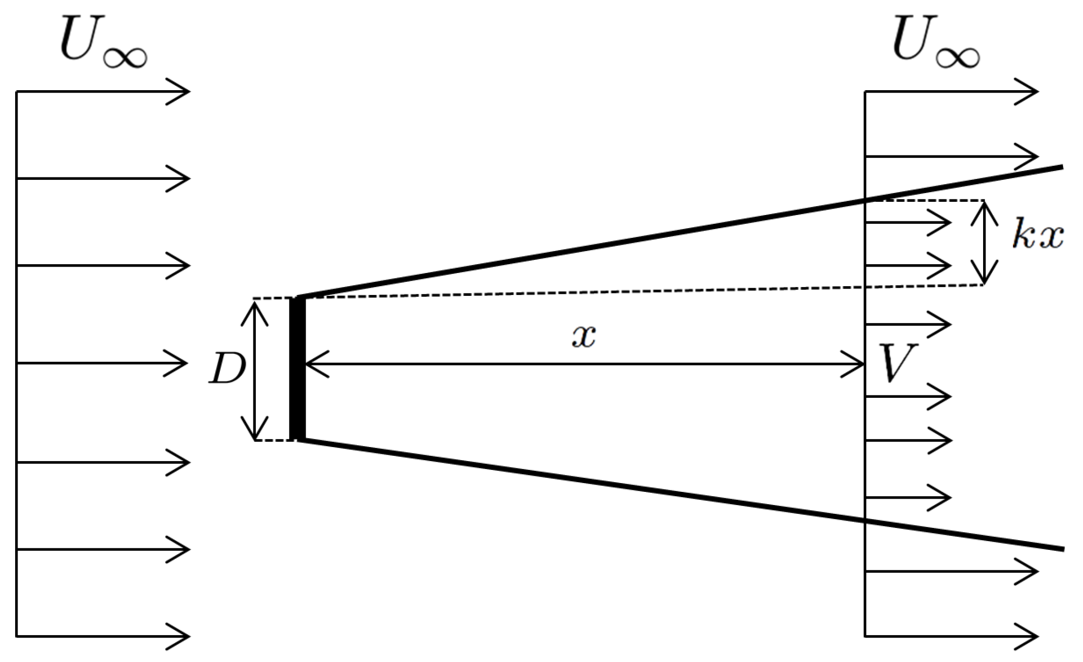
Two analytical wake models are used in this study, the Jensen [4] and the Larsen [5]. The Jensen model is based on the description of a single wake behind a rotor. Here the normalized wind velocity deficit as presented in [6] is used δ U = U V U , at a distance x behind a single wind turbine with a thrust coefficient C T is found by
δ U = 1 1 C T 1 + 2 k x D 2 ,
where k is the wake expansion coefficient, D the rotor diameter of the wind turbine and V the wind velocity in the wake at position x (Figure 2). The wake expansion coefficient k is found by k = A j ln ( z h / z 0 ) . Where A j is a constant equal to A j = 0.5 , z h the wind turbine hub height and z 0 is the effective roughness height. When multiple wakes influence the velocity at a position, the total normalized velocity deficit δ U t o t . , is found by
δ U t o t . = δ U j 2 ,
where δ U j is the normalized wind velocity deficit from the j-th wind turbine.
The Larsen model is based on turbulent boundary layer equations and a similarity assumption. By neglecting different terms in the governing equations, two different versions of the model are presented in [5]. Here we will be using the first order wake model in which the normalized velocity deficit is described by
δ U = C T A x 2 1 / 3 9 r x 3 / 2 3 c 1 2 C T A x 1 / 2 35 2 π 3 / 10 3 c 1 2 1 / 5 2 ,
where r x is the radial distance at a position x downstream of the rotor and c 1 is a computed parameter. The parameter c 1 is found by
c 1 = D 2 5 / 2 C T A x 0 5 / 6 ,
where
x 0 = 9.5 D ( 2 R 95 / D ) 3 1 ,
R 95 = 0.5 R n b min ( z h , R n b ) ,
R n b = max 1.08 D , 1.08 D + 21.7 D ( T I h 0.05 ) .
T I h is the ambient turbulence intensity at hub height ( z h ), R n b is a constant dependent on the rotor diameter and the ambient turbulence intensity at hub height. A notable difference between the Jensen and Larsen models is that the wake deficit for the Larsen model is not uniform, as is the case for the Jensen model, but differs radially in the cross-section of the wake, due to r x . The effect of multiple wakes on the velocity field at a position is also taken into account by Equation (7).
The power production at each wind turbine is found by the velocity at hub height minus the velocity deficit calculated by either the Jensen or Larsen wake model.

2.3. Boundary Conditions

The simulations are performed by the commercial CFD code WindSim. The RANS equations are solved via a general collocated velocity method (GCV) [34] in a body-fitted coordinate grid formulation (BFC). Therefore, the variables are stored on a collocated mesh. The GCV method, however, uses a segregated pressure-based solver strategy, thus a momentum interpolation algorithm is performed to evaluate mass fluxes on the control volume faces. This algorithm is a variant of the Rhie–Chow momentum interpolation method [35,36], which avoids the undesired side effect of producing solutions that depend on the relaxation factors used [37]. The k ε two equation turbulence model is used to close the equations. Full mathematical formulation of the model can be found in [38], whereas a detailed description of the computational domain and mesh can be found in Section 2.3.1. The hybrid method of [39] is used to discretize the convective terms. The diffusion terms, on the other hand, are discretized by using the central differencing scheme. At the inlet of the domain, a log law velocity profile is set with the turbulence parameters obeying the following equations
U ( z ) = U i * κ ln z z 0 , k = U i * 2 0.3 and ε = U i * 3 κ z ,
where U ( z ) is the streamwise wind velocity at height z, U i * is the inlet friction velocity, κ is von Kármán’s constant set to 0.41, z 0 is the effective roughness height, k is the turbulent kinetic energy and ε is the dissipation rate. The ambient turbulence intensity at hub height ( T I h ) assuming an isotropic normal stress approximation is given by
T I h = 2 3 k U h T I h = κ 2 3 ln z h z 0 C μ 4 ,
where U h is the streamwise wind velocity at hub height z h and C μ is an empirical constant equal to 0.09. This value for C μ was recommended by [40] after researching free turbulent flows. By knowing the values for the turbulence intensity at hub height (see Section 3), using Equation (14) the appropriate value for the effective roughness height ( z 0 ) is found. The wall function of the ground surface is described by the following equations
U r = U w * κ ln z r z 0 , k = U w * 2 0.3 and ε = C μ 0.75 k 1.5 κ z r ,
where U r is the absolute value of the velocity parallel to the wall at the first grid node and z r is the normal distance of the first grid node from the wall. Here the wall friction velocity U w * is calculated from U w * = τ w / ρ , the wall shear stress is τ w = s ρ U r 2 and s = κ ln z r z 0 2 . The lateral walls of the domain are impermeable and frictionless. The outlet and top plane are treated as a fixed pressure boundary. Moreover, a diffusive link is set at the top plane to help preserve the inlet boundary profile calculated via Equation (13) ([41]). The pressure value at the outlet is set to zero.

2.3.1. Body-Fitted Grid

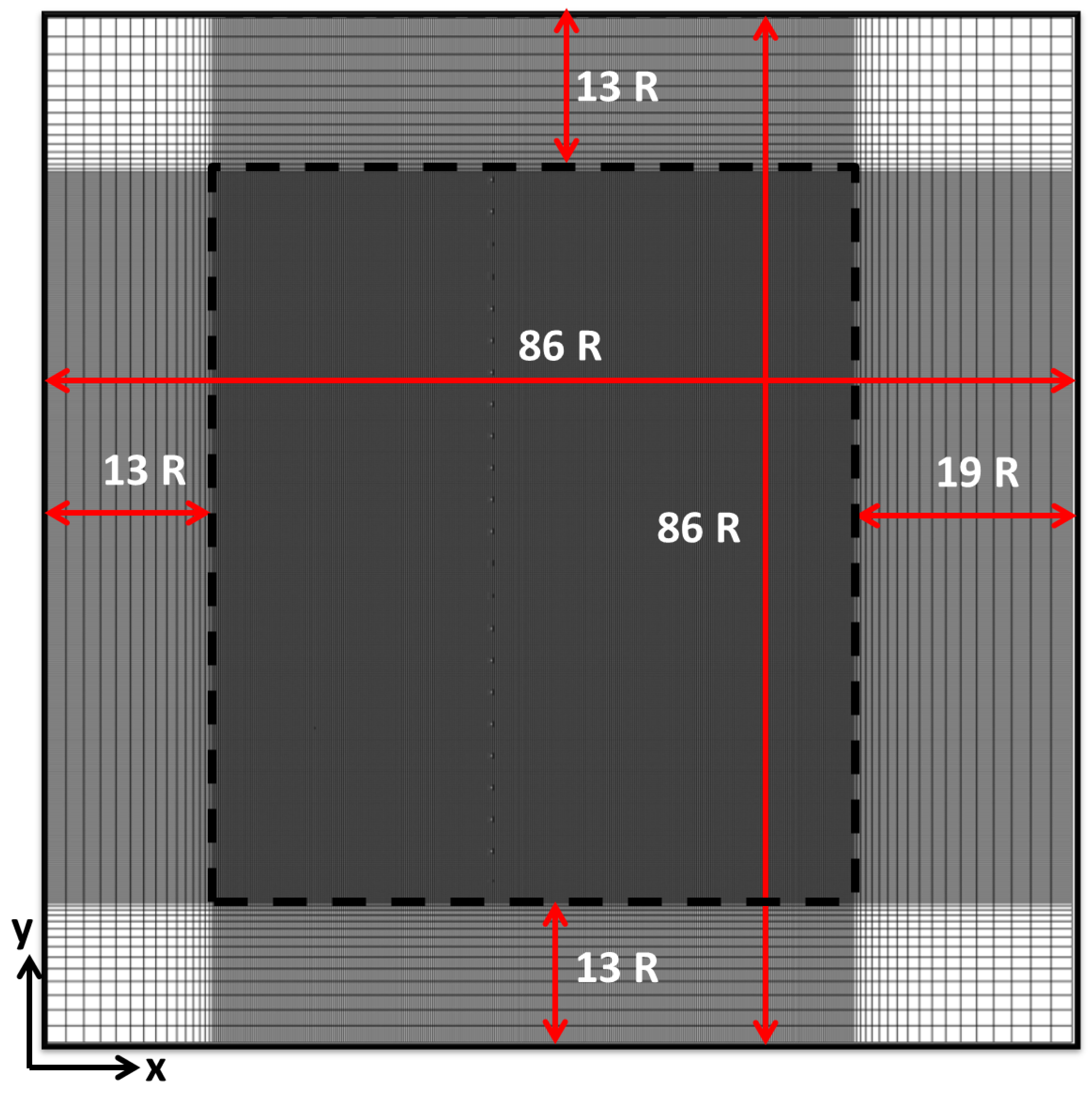
A top view of the body-fitted grid used within this study is presented at ground level in Figure 3. The grid is composed of topologically six-sided control volumes/cells. The domain used for the simulation has dimensions of ( x , y , z ) = ( 86 R , 86 R , 11 R ) . An inner equidistant region (within the dashed box Figure 3) with a cell size of R/6 is defined for the domain containing the ACDs, while outside this equidistant region the resolution expands. The equidistant region is automatically defined by the software after the wind turbine locations are selected. The total number of cells is approximately 3.8 million. Table 2 presents the main parameters of the domain, R is the rotor radius and ( L x , L y , L z ), ( l x , l y , l z ) are respectively the length of the domain and inner equidistant region.

3. Lillgrund Offshore Wind Farm

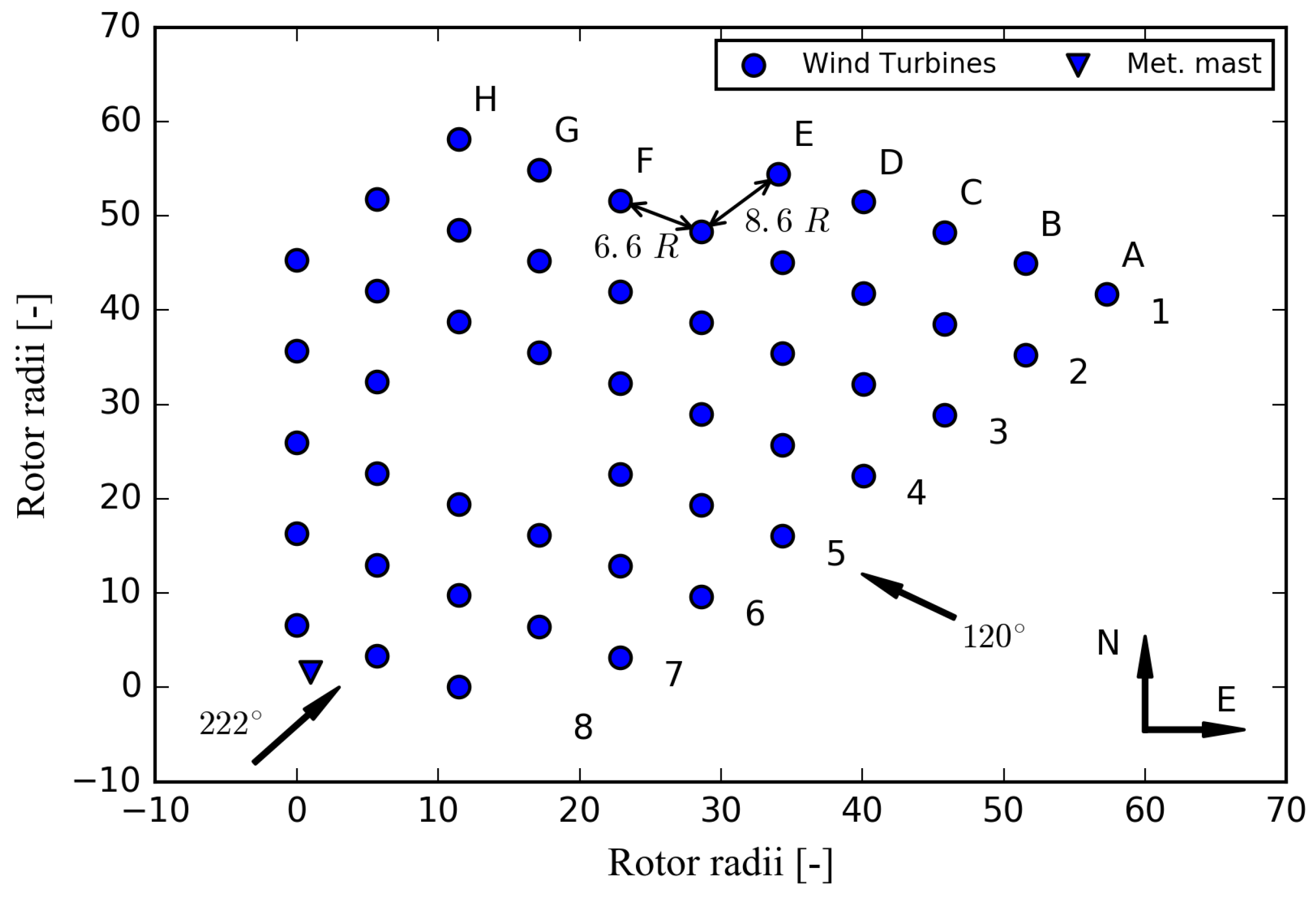
The total rated power of the Lillgrund wind farm is 110.4 MW which consists of 48 Siemens SWT-2.9-93 wind turbines with a rated power of 2.3 MW each. The rotor diameter of the Siemens SWT-2.9-93 wind turbine is 92.6 m and the hub height is at 65 m. The wind farm layout is shown in Figure 4. The convention used herein to label each individual wind turbine is to assign them a letter and number, the letter represents the column in which the wind turbine is located ranging from A–H and the number represents the appointed row ranging from 1–8. A distinct feature of the Lillgrund wind farm is the very tight configuration of the wind turbines, with a separation distance of 6.6 rotor radii (R), for the columns and 8.6 R for the rows. The reason behind this unusually compact inter–row spacing according to [42] is that the layout was initially developed for a smaller wind turbine model. This model was however unavailable when the construction permit for the wind farm was finally given. As a result, the developers decided to use a larger wind turbine while keeping the original layout. Another noteworthy feature of this layout is the gap in the middle of the farm where wind turbines D5 and E5 should have been placed. This gap increases the separation distance locally and will influence the total wake recovery and power production of the wind turbines downstream of the gap.
The turbulence intensity per direction used in this study was estimated by data extracted from a met mast, located to the south–west as seen in Figure 4, during approximately a two-year period prior to the erection of the wind turbines (1st of September 2013 to the 28th of February 2016) [43]. The inflow directions on which this study will focus are shown in Table 3 along with the respective turbulence intensities at a 65 m height. Specifically, for the wind flow direction of 120 ° , data are used from rows 3 and 5 at a wind velocity of 9 m s 1 . Similarly, for the 222 ° inflow direction, data are used from column B and D at a wind velocity of 9 m s 1 . Rows 3, 5 and columns B, D have been selected because they represent two distinct cases in which one row/column includes the gap and the other does not (Figure 4).
Records from the wind turbines’ SCADA system are available for 10 min time periods. The power production of each wind turbine per inflow direction and undisturbed wind speed is thus available. Due to data availability limitations the power production data are binned based on inflow directions and wind velocity measurements. The directional bins are ± 2.5 ° wide and the velocity bins are ± 0.5 m s 1 wide as seen in Table 3 below.
The inflow wind direction is calculated by the average wind turbine yaw position from a group of wind turbines. For the 120 ° direction, the group of wind turbines consists of turbines A1 to A7; similarly, for the 222 ° direction the wind turbines B8 to D8 are used. The undisturbed wind velocity used per direction is derived by averaging the undisturbed wind velocity of all wind turbines in the noted groups. The undisturbed velocity of each wind turbine in the group is found by comparing the 10 min power production of the turbine to the official power curve as found in [33]. It should be noted, that for these data a filtration depending on the atmospheric stability condition has not been performed.

4. Results and Discussion

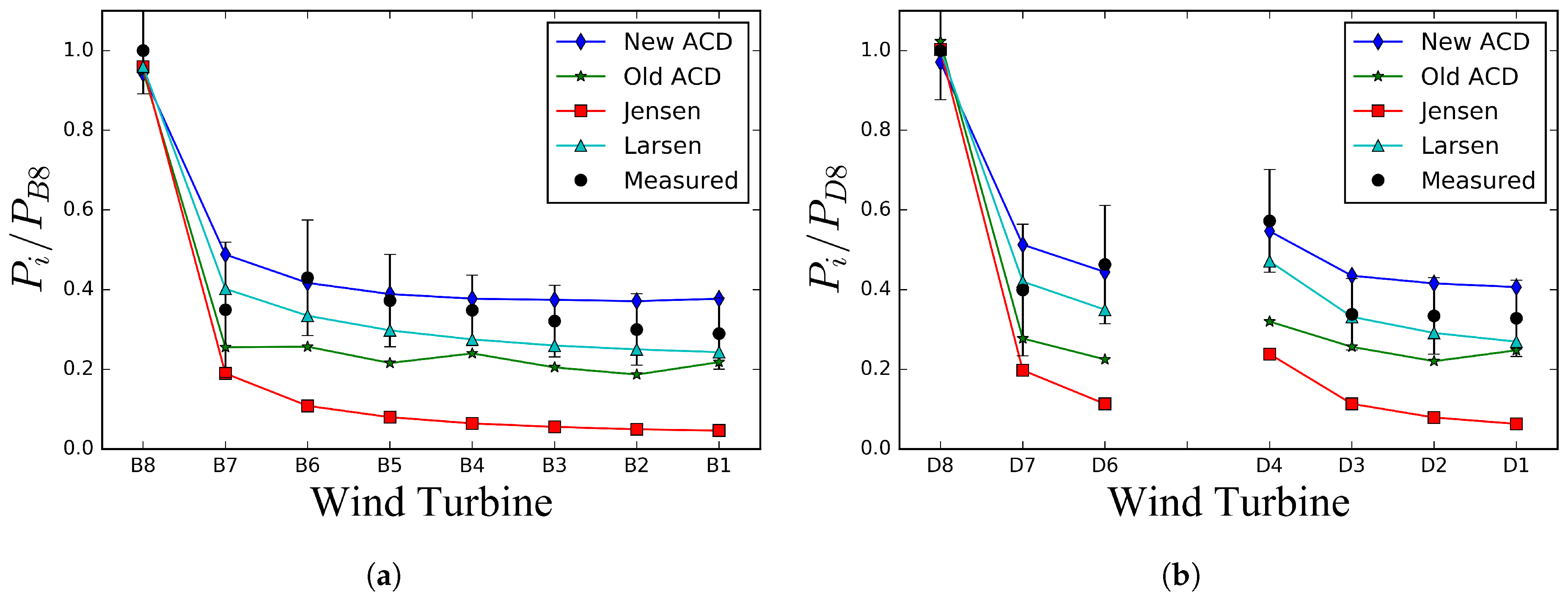
Results of the comparative analysis will be presented in this section after normalization. The normalization is done by dividing the power production of each wind turbine of the row/column with the measured power production of the first wind turbine in the row/column. The reported error bar range is equal to the normalized standard deviation of the measured power production.
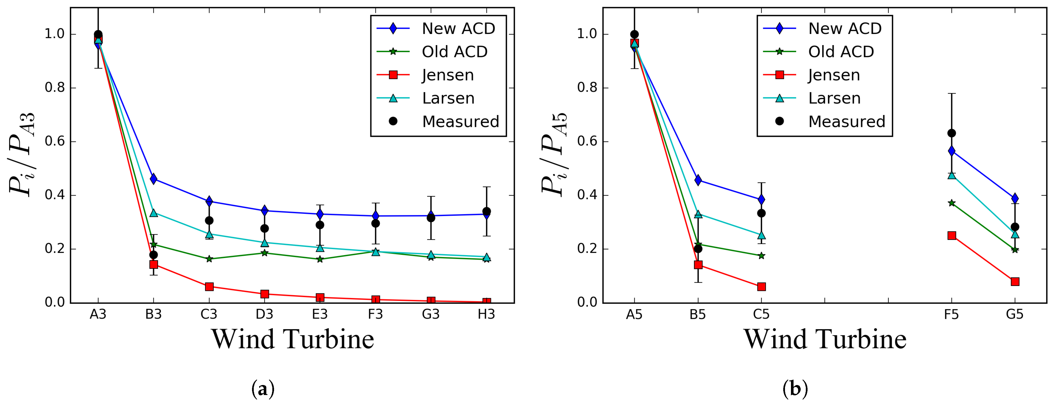
Figure 5 below presents the results of Row 3 and 5 for the 120 ° wind direction. It is observed that the power production of the first wind turbine is captured by all methods/models. Regarding the second wind turbine of the row, however, the ACD (2016) method and the Larsen model do not capture the steep reduction of the measured power output. In contrast, the ACD (2008) method and the Jensen model give results within the error range. The power production of the third wind turbine is captured within the error range when using the ACD (2016) and the Larsen model, which is not the case for the ACD (2008) and the Jensen model. None of the methods/models can capture the sharp power production increase observed in the measurements from the second to the third wind turbine. The power production of the subsequent wind turbines in Figure 5a is captured within good accuracy when using the ACD (2016) method, whereas the other method/models underestimate the power production. Regarding Figure 5b, the increase of the power output observed between the C5 and F5 wind turbines due to the gap, is captured best by the ACD (2016) method.
Other researchers have also studied the Lillgrund wind farm case. Researchers in [44] used the k ε and the k ε f p turbulence models to investigate their effects on the simulated power production for rows 3 and 5. Their results with the k ε turbulence model coincide with the ones presented here for the ACD (2016) method case. On the other hand, the k ε f p made better predictions of the power production, especially for the second wind turbine in the row. Furthermore, other scholars have used LES with an ACD method to simulate power production for the same wind turbines rows of the Lillgrund wind farm [23]. Their simulations predicted with better accuracy the power production of the same wind turbine rows including the power deficit of the second wind turbine and the power increase between the C5 and the F5 wind turbines. That is expected since LES fully resolves the effect of the large turbulent eddies.
Results of columns B and D for the 222 ° wind direction case are presented in Figure 6.
Here again the ACD (2016) method and the Larsen model over–predict the power production of the second wind turbine, whereas the ACD (2008) and the Jensen model under–predict the power production. It is known from literature that ACD models generally perform poorly in the near wake of a wind turbine [25]. For the Lillgrund wind farm with its exceptionally close spacing, this might impact the accuracy of the results. The second wind turbine in the row/column can be considered lying in the near wake region and this could explain the over–prediction of the method. For the remaining wind turbines in the rows the ACD (2016) method and the Larsen model outperform the ACD (2008) method and the Jensen model. In another study, [11], in which the focus of the comparative analysis was on the wind turbines positioned in column C for a main wind direction of 222 ° at a wind speed of 8 ± 0.5 m s 1 , it was found that the three wake models [4,9,10] performed similarly for the Lillgrund case. Here we find that the Larsen wake model in general outperforms the Jensen wake model. This highlights the complexity of this type of analysis. One may argue that it should not be expected that similar conclusions would be found when investigating different columns/rows (with or without a gap in between turbines in this case) of wind turbines, wind velocities and slightly different wake models. In that sense similar studies such as the ones performed by [11,13,14,23,44,45,46] may complement each other. In addition, they highlight the strengths and limitations of each model/method and offer to researchers better possibilities to gain a deeper and more integrated insight into the particular usefulness of every model/method under different circumstances and cases.
Results similar to those of the ACD (2016) method presented here when using the k ε turbulence model were obtained in [44]. In addition, they showed that their results improved with the k ε f p turbulence model. In [44,47] it was shown with wind measurements and LES that the k ε turbulence closure model is not capable of replicating wakes of isolated wind turbines. Specifically, the k ε turbulence closure model, under–predicts the wake effects due to it being too diffusive. Here the goal is not to investigate the influence of the effect of using different turbulence closer models, rather we are interested in a comparative analysis of two ACD methods and two analytical wake models for a wind farm configuration. Moreover, LES with an ACD and ACL method have been performed by [14,23] respectively, with quite good accuracy. The researchers in [23] have generally slightly over predicted the measurements whereas results of [14] vary depending on the particular wind turbine examined.
While this study has provided a clear comparison between the ACD (2016) and ACD (2008) actuator disc methods and two analytical wake models with experimental data, it is also important to mention its limitations:
  • When presenting the results, the directional uncertainty as proposed by [48] has not been considered.
  • Yaw misalignment errors are not considered.
  • The data has not been filtered for stability.
  • The study has been performed only for cases where the wind direction is in-line to the row of wind turbines.
  • Only the k ε turbulence model is used.
  • In the simulations one power curve is used; in reality depending on the environmental conditions e.g., turbulence intensity or air density, wind turbines operate on a range of power curves.
Despite these limitations, the present study has presented a straightforward comparison among different methods to estimate the power production of a wind farm. Even though the ACDs used in this study are both based on the 1D momentum theory, it is shown that they provide different results as a consequence of how the forces are calculated and distributed over the disc and how the power is estimated. The ACD (2016) method and the Larsen model, in most cases, seem to better estimate the power production in comparison to the other method and model. The Jensen model in particular seems in general to greatly underestimate the power production of the downwind turbines.

5. Conclusions

This paper compared the power production results of four different methods/models against measurements for the offshore wind farm of Lillgrund, which is in Sweden. Two ACD methods based on the 1D momentum theory are compared along with two analytical wake models, the Jensen and the Larsen. For this comparison two main wind directions are investigated. The main conclusions are: (i) The ACD (2016) method and the Larsen model outperform the other method and model in most cases. (ii) The power increase of the turbine after the gap is better captured when using the ACD (2016) method. (iii) The results from the ACD (2016) method show a clear improvement in the estimated power production in comparison to the ACD (2008) method. (iv) The Jensen method seems to overestimate the power deficit for all cases. (iv) The ACD (2016) method, despite its simplicity, can capture the power production within the error margin although it tends to underestimate the power deficit. One may say that the ACD (2016) method in RANS, which has much lower computational requirements than the ACD method in LES at the cost of lower accuracy, could represent a good compromise.
It should be noted that the ACD (2008) approach uses a simplified approach to calculate the power production of the wind turbine, that is the wind velocity at hub height. The ACD methods presented in [20,49] on the other hand use an average of the wind speed over the rotor. As such, it would be interesting for a future study to include a more advanced ACD method in a comparison study with the ACD (2016).
Additionally, [44] showed that by using the k ε f p turbulence model the power production results for the second wind turbine in the row are in closer agreement with the measurements than when using the k ε model. Hence future work could focus on researching the impact of using different turbulence closure models on the results. Also, as the Lillgrund wind farm is quite unique due to its very close inter-row spacing of the wind turbines, it would be advantageous to apply a similar comparative analysis using these methods/models on wind farms with larger distances between wind turbines. Furthermore, as stability has an impact on wake development it is important to explore wind farm cases in which the data can be filtered for stability. Finally, it would prove beneficial to continue investigating the offshore Lillgrund wind farm for other wind flow conditions to obtain a more comprehensive understanding of the performance of the methods/models.

Author Contributions

N.S.: Conceptualization, Formal analysis, Methodology, Software, Validation, Writing—original draft, Writing—review & editing, Corresponding author. H.P.: Conceptualization, Supervision, Visualization, Writing—original draft, Writing—review & editing. S.I.: Funding acquisition, Project administration, Resources, Supervision. All authors have read and approved the final version of the paper.

Funding

This research was funded by the Research Council of Norway (Project no. 231831).

Acknowledgments

The filtration and validation of the data was performed by Kurt Schaldemose Hansen (DTU Institute for Vindenergy Denmark) according to the guidelines described in [50]. Andrew Barney is kindly acknowledged for proof reading the manuscript.

Conflicts of Interest

The authors declare no conflict of interest.

Abbreviations

The following abbreviations are used in this manuscript:
ACDActuator Disc
ACLActuator Line
RANSReynolds Averaged Navier–Stokes
LESLarge Eddy Simulations
GCVGeneral Collocated Velocity
BFCbody-fitted Coordinate

References

  1. Polatidis, H.; Ivanell, S. Micro-siting/positioning of wind turbines: Introducing a multi-criteria decision analysis framework. In Proceedings of the 7th International Multi-Conference on Engineering and Technological Innovation (IMETI 2014), Orlando, FL, USA, 15–18 July 2014; pp. 23–27. [Google Scholar]
  2. Barthelmie, R.J.; Hansen, K.; Frandsen, S.T.; Rathmann, O.; Schepers, J.; Schlez, W.; Phillips, J.; Rados, K.; Zervos, A.; Politis, E.; et al. Modelling and measuring flow and wind turbine wakes in large wind farms offshore. Wind Energy 2009, 12, 431–444. [Google Scholar] [CrossRef]
  3. Hou, P.; Hu, W.; Soltani, M.; Chen, C.; Chen, Z. Combined optimization for offshore wind turbine micro siting. Appl. Energy 2017, 189, 271–282. [Google Scholar] [CrossRef]
  4. Jensen, N.O. A Note on Wind Generator Interaction; Technical University of Denmark: Kongens Lyngby, Denmark, 1983. [Google Scholar]
  5. Larsen, G.C. A Simple Wake Calculation Procedure; Technical University of Denmark: Kongens Lyngby, Denmark, 1988. [Google Scholar]
  6. Katic, I.; Højstrup, J.; Jensen, N. A Simple Model for Cluster Efficiency. In Proceedings of the European Wind Energy Association Conference and Exhibition, Rome, Italy, 7–9 October 1986. [Google Scholar]
  7. Troldborg, N. Actuator Line Modeling of Wind Turbine Wakes; Technical University of Denmark: Kongens Lyngby, Denmark, 2009. [Google Scholar]
  8. Seim, F.; Gravdahl, A.R.; Adaramola, M.S. Validation of kinematic wind turbine wake models in complex terrain using actual windfarm production data. Energy 2017, 123, 742–753. [Google Scholar] [CrossRef]
  9. Larsen, G.C. A Simple Stationary Semi-Analytical Wake Model; Technical University of Denmark: Kongens Lyngby, Denmark, 2009. [Google Scholar]
  10. Ott, S.; Berg, J.; Nielsen, M. Linearised CFD Models for Wakes; Risø National Laboratory: Roskilde, Denmark, 2011.
  11. Gaumond, M.; Réthoré, P.E.; Bechmann, A.; Ott, S.; Larsen, G.C.; Pena Diaz, A.; Kurt, K. Benchmarking of wind turbine wake models in large offshore windfarms. In Proceedings of the Science of Making Torque from Wind 2012 Conference, Oldenburg, Germany, 9–11 Octorber 2012. [Google Scholar]
  12. Silicon Graphics International Corporation. OpenFOAM. Available online: http://www.openfoam.org (accessed on 13 December 2018).
  13. Rolf-Erik, K. Validation of the standalone implementation of the dynamic wake meandering model for power production. Wind Energy 2015, 18, 1579–1591. [Google Scholar]
  14. Churchfield, M.; Lee, S.; Moriarty, P.; Martinez, L.; Leonardi, S.; Vijayakumar, G.; Brasseur, J. A large-eddy simulations of wind-plant aerodynamics. In Proceedings of the 50th AIAA Aerospace Sciences Meeting including the New Horizons Forum and Aerospace Exposition, Nashville, TN, USA, 9–12 January 2012; p. 537. [Google Scholar]
  15. Sørensen, J.N.; Shen, W.Z. Numerical modeling of wind turbine wakes. J. Fluids Eng. 2002, 124, 393–399. [Google Scholar] [CrossRef]
  16. Ivanell, S.; Sørensen, J.N.; Mikkelsen, R.; Henningson, D. Numerical analysis of the tip and root vortex position in the wake of a wind turbine. J. Phys. Conf. Ser. 2007, 75, 012035. [Google Scholar] [CrossRef] [Green Version]
  17. Nilsson, K.; Shen, W.Z.; Sørensen, J.N.; Breton, S.P.; Ivanell, S. Validation of the actuator line method using near wake measurements of the MEXICO rotor. Wind Energy 2015, 18, 499–514. [Google Scholar] [CrossRef]
  18. Sarmast, S.; Dadfar, R.; Mikkelsen, R.F.; Schlatter, P.; Ivanell, S.; Sørensen, J.N.; Henningson, D.S. Mutual inductance instability of the tip vortices behind a wind turbine. J. Fluid Mech. 2014, 755, 705–731. [Google Scholar] [CrossRef] [Green Version]
  19. Breton, S.P.; Nilsson, K.; Olivares-Espinosa, H.; Masson, C.; Dufresne, L.; Ivanell, S. Study of the influence of imposed turbulence on the asymptotic wake deficit in a very long line of wind turbines. Renew. Energy 2014, 70, 153–163. [Google Scholar] [CrossRef]
  20. Wu, Y.T.; Porté-Agel, F. Large-eddy simulation of wind-turbine wakes: Evaluation of turbine parametrisations. Bound. Layer Meteorol. 2011, 138, 345–366. [Google Scholar] [CrossRef]
  21. Olivares-Espinosa, H.; Breton, S.; Masson, C.; Dufresne, L. Turbulence characteristics in a free wake of an actuator disk: comparisons between a rotating and a non-rotating actuator disk in uniform inflow. J. Phys. 2014, 555, 012081. [Google Scholar] [CrossRef] [Green Version]
  22. Van der Laan, M.P.; Sørensen, N.N.; Réthoré, P.E.; Mann, J.; Kelly, M.C.; Troldborg, N.; Schepers, J.G.; Machefaux, E. An improved k-ε model applied to a wind turbine wake in atmospheric turbulence. Wind Energy 2015, 18, 889–907. [Google Scholar] [CrossRef]
  23. Nilsson, K.; Ivanell, S.; Hansen, K.S.; Mikkelsen, R.; Sørensen, J.N.; Breton, S.P.; Henningson, D. Large-eddy simulations of the Lillgrund wind farm. Wind Energy 2015, 18, 449–467. [Google Scholar] [CrossRef]
  24. Castellani, F.; Vignaroli, A. An application of the actuator disc model for wind turbine wakes calculations. Appl. Energy 2013, 101, 432–440. [Google Scholar] [CrossRef]
  25. Prospathopoulos, J.; Politis, E.; Rados, K.; Chaviaropoulos, P. Evaluation of the effects of turbulence model enhancements on wind turbine wake predictions. Wind Energy 2011, 14, 285–300. [Google Scholar] [CrossRef]
  26. El Kasmi, A.; Masson, C. An extended k–ε model for turbulent flow through horizontal-axis wind turbines. J. Wind Eng. Ind. Aerodyn. 2008, 96, 103–122. [Google Scholar] [CrossRef]
  27. Sumner, J.; Espana, G.; Masson, C.; Aubrun, S. Evaluation of RANS/actuator disk modelling of wind turbine wake flow using wind tunnel measurements. Int. J. Eng. Syst. Model. Simul. 2013, 5, 147–158. [Google Scholar] [CrossRef]
  28. Crasto, G.; Gravdahl, A.R. CFD wake modeling using a porous disc. In Proceedings of the European Wind Energy Conference & Exhibition 2008, Brussels, Belgium, 31 March–3 April 2008. [Google Scholar]
  29. WindSim AS. 2017. Available online: https://windsim.com (accessed on 14 December 2018).
  30. Simisiroglou, N.; Sarmast, S.; Breton, S.P.; Ivanell, S. Validation of the actuator disc approach in PHOENICS using small scale model wind turbines. J. Phys. 2016, 753, 032028. [Google Scholar] [CrossRef] [Green Version]
  31. Calaf, M.; Meneveau, C.; Meyers, J. Large eddy simulation study of fully developed wind-turbine array boundary layers. Phys. Fluids 2010, 22, 015110. [Google Scholar] [CrossRef] [Green Version]
  32. Hansen, K. Presentation of Lillgrund Offshore Wind Farm and the Siemens SWT-2.3-93 Wind Turbine; Siemens: Munich, Germany, 2013. [Google Scholar]
  33. Jeppsson, J.; Larsen, P.E.; Larsson, Å. Technical Description Lillgrund Wind Power Plant; Vattenfall Vindkraft: Stockholm, Sweden, 2008; 78p. [Google Scholar]
  34. Semin, V.; Spalding, D.; Zhubrin, S. Two novel algorithms for the simulation of flow around turbine blades. In IMechE Seminar “Latest Advances in the Aerodynamics of Turbomachinery with Special Emphasis on Unsteady Flows”; Professional Engineering Publishing: London, UK, 1996. [Google Scholar]
  35. Rhie, C.M. Numerical study of the flow past an isolated airfoil with separation. Diss. Abstr. Int. Part B Sci. Eng. 1982, 42, 3793. [Google Scholar]
  36. Rhie, C.; Chow, W.L. Numerical study of the turbulent flow past an airfoil with trailing edge separation. AIAA J. 1983, 21, 1525–1532. [Google Scholar] [CrossRef]
  37. Majumdar, S. Role of underrelaxation in momentum interpolation for calculation of flow with nonstaggered grids. Numer. Heat Transf. 1988, 13, 125–132. [Google Scholar] [CrossRef]
  38. Launder, B.E.; Spalding, D. The numerical computation of turbulent flows. Comput. Methods Appl. Mech. Eng. 1974, 3, 269–289. [Google Scholar] [CrossRef]
  39. Spalding, D. A novel finite difference formulation for differential expressions involving both first and second derivatives. Int. J. Numer. Methods Eng. 1972, 4, 551–559. [Google Scholar] [CrossRef]
  40. Launder, B.; Morse, A.; Rodi, W.; Spalding, D. Prediction of Free Shear Flows: A Comparison of the Performance of Six Turbulence Models; NASA: Washington, DC, USA, 1973.
  41. PHOENICS VR Reference Guide TR326. 2017. Available online: http://www.cham.co.uk/documentation/tr326.pdf (accessed on 14 December 2018).
  42. Dahlberg, J.A. Assessment of the Lillgrund Wind Farm: Power Performance Wake Effects. Available online: https://corporate.vattenfall.se/globalassets/sverige/om-vattenfall/om-oss/var-verksamhet/vindkraft/lillgrund/assessment.pdf (accessed on 14 December 2018).
  43. Bergström, H. Meteorological conditions at Lillgrund. Vattenfall Vindkraft AB 2009. Available online: https://corporate.vattenfall.se/globalassets/sverige/om-vattenfall/om-oss/var-verksamhet/vindkraft/lillgrund/meteorological_conditions.pdf (accessed on 14 December 2018).
  44. Van der Laan, M.P.; Sørensen, N.N.; Réthoré, P.E.; Mann, J.; Kelly, M.C.; Troldborg, N.; Hansen, K.S.; Murcia, J.P. The k-ε-fP model applied to wind farms. Wind Energy 2015, 18, 2065–2084. [Google Scholar] [CrossRef]
  45. Pena, A.; Réthoré, P.E.; Hasager, C.B.; Hansen, K.S. Results of Wake Simulations at the Horns Rev I and Lillgrund Wind Farms Using the Modified Park Model; Technical University of Denmark: Kongens Lyngby, Denmark, 2013. [Google Scholar]
  46. Creech, A.C.; Früh, W.G.; Maguire, A.E. High-resolution CFD modelling of Lillgrund Wind farm. In Proceedings of the International Conference on Renewable Energies and Power Quality, Bilbao, Spain, 20–22 March 2013. [Google Scholar]
  47. Réthoré, P.E. Wind Turbine Wake in Atmospheric Turbulence. Ph.D. Thesis, Aalborg University, Aalborg, Denmark, 2009. [Google Scholar]
  48. Gaumond, M.; Réthoré, P.E.; Ott, S.; Peña, A.; Bechmann, A.; Hansen, K.S. Evaluation of the wind direction uncertainty and its impact on wake modeling at the Horns Rev offshore wind farm. Wind Energy 2014, 17, 1169–1178. [Google Scholar] [CrossRef]
  49. Van der Laan, M.P.; Sørensen, N.N.; Réthoré, P.E.; Mann, J.; Kelly, M.C.; Troldborg, N. The k-ε-fP model applied to double wind turbine wakes using different actuator disk force methods. Wind Energy 2015, 18, 2223–2240. [Google Scholar] [CrossRef]
  50. Barthelmie, R.J.; Frandsen, S.T.; Rathmann, O.; Hansen, K.S.; Politis, E.; Prospathopoulos, J.; Schepers, J.; Rados, K.; Cabezón, D.; Schlez, W.; et al. Flow and Wakes in Large Wind Farms: Final Report for UpWind WP8; Technical University of Denmark: Kongens Lyngby, Denmark, 2011. [Google Scholar]
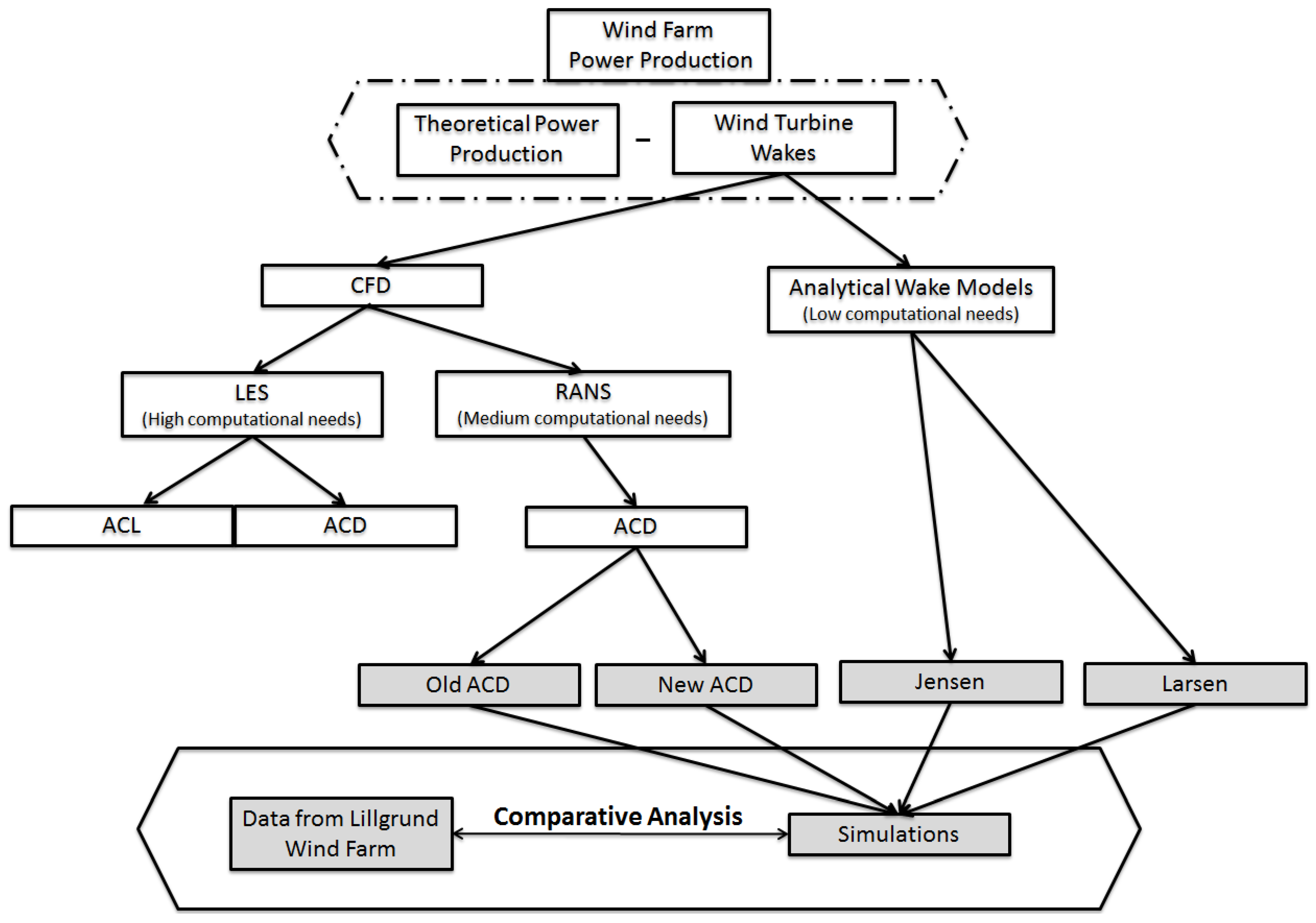
Figure 1. Methodological framework.
Applsci 09 00431 g001
Figure 2. Schematic representation of the Jensen wake model. (D is the rotor diameter, U the undisturbed wind velocity, x the downstream distance of the wake from the rotor, V the velocity within the wake and k the wake expansion coefficient).
Applsci 09 00431 g002
Figure 3. Top view of WindSim generated mesh. (Grid resolution at ground level, R is the wind turbine radius).
Applsci 09 00431 g003
Figure 4. Layout of Lillgrund wind farm, where R is the rotor radius. 120 ° and 222 ° are the inflow directions to be investigated.
Applsci 09 00431 g004
Figure 5. Normalized power production for the 120 ° direction (a) Row 3 and (b) Row 5.
Applsci 09 00431 g005
Figure 6. Normalized power production for the 222 ° direction (a) Column B and (b) Column D.
Applsci 09 00431 g006
Table 1. Main differences between the ACD (2008) and the ACD (2016) methods.
DescriptionPower Production EstimationThrust CoefficientThrust Distribution
ACD (2008)Velocity at hub height C T staticUniform, Parabolic and Polynomial
ACD (2016)Averaged value over the rotor C T ( U d , i ) update at each iterationUndistributed
Table 2. Domain set-up.
DomainInner Equidistant RegionTotal Number of Cells
Lx Ly Lz lx ly lz Cell Size
86 R 86 R 11 R 54 R 60 R 5 R R / 6 3.4 × 10 6
Table 3. Main inflow directions and information.
DescriptionInflow Direction (Degrees)Row/ColumnWind Velocity (m s 1 )Turbulence Intensity (%)
Southeast 120 ± 2.5 ° 3, 5 9.0 ± 0.5 5.5
Southwest 222 ± 2.5 ° B, D 9.0 ± 0.5 5.6