Abstract
Reliable prediction of remaining useful life (RUL) plays an indispensable role in prognostics and health management (PHM) by reason of the increasing safety requirements of industrial equipment. Meanwhile, data-driven methods in RUL prognostics have attracted widespread interest. Deep learning as a promising data-driven method has been developed to predict RUL due to its ability to deal with abundant complex data. In this paper, a novel scheme based on a health indicator (HI) and a hybrid deep neural network (DNN) model is proposed to predict RUL by analyzing equipment degradation. Explicitly, HI obtained by polynomial regression is combined with a convolutional neural network (CNN) and long short-term memory (LSTM) neural network to extract spatial and temporal features for efficacious prognostics. More specifically, valid data selected from the raw sensor data are transformed into a one-dimensional HI at first. Next, both the preselected data and HI are sequentially fed into the CNN layer and LSTM layer in order to extract high-level spatial features and long-term temporal dependency features. Furthermore, a fully connected neural network is employed to achieve a regression model of RUL prognostics. Lastly, validated with the aid of numerical and graphic results by an equipment RUL dataset from the Commercial Modular Aero-Propulsion System Simulation(C-MAPSS), the proposed scheme turns out to be superior to four existing models regarding accuracy and effectiveness.
1. Introduction
The complexity of the equipment involved in modern industry has rapidly increased in the past decades [1]. Any failure of equipment may cause catastrophic consequences [2,3], and reliability and maintenance are key for equipment [4]. Therefore, it’s essential to have an effective strategy that positively coordinates scheduling and maintenance to ensure productivity, personal safety and manufacturing development [5].
Prognostics and health management (PHM) is a key technology that can guarantee the security of equipment and reduce maintenance costs [6]. As a crucial component of PHM, remaining useful life (RUL) prediction has evolved into an active research field due to its enhanced capability to determine the maintenance time [7]. RUL of equipment is defined as the length from the current time to the end of the useful life [8]. RUL prognostics approaches consist of model-based, data-driven, and fusion prognostics [9]. More particularly, model-based methods describe equipment health state by modeling the degradation evolution of physical structure. Unfortunately, model-based methods are constrained in adapting complex equipment structure [10]. Ideally, data-driven methods put to use sensor measurement data or operational data to predict RUL without foreknowledge of the physical structure and the degradation mechanism [11]. Additionally, the above-mentioned model-based methods and data-driven methods are combined into fusion prognostics methods [9]. However, very few studies about fusion prognostics methods have been reported, due to the undiscovered intricacy of the physical structure [12,13]. Actually, data-driven methods have been proven to be capable of predicting RUL in extensive research [14,15].
Over the years, since sensor measurement data are intrinsically of the time series nature, the mainstream data-driven research in the field of RUL prognostics focuses on prediction techniques based on sequence learning [8]. In previous research, a large number of machine learning approaches have been proposed, most of which construct prognostics models by analyzing correlative sensor sequential data and associating the discovered hierarchical patterns with a definite prognostics task [16]. These prediction models provide effective evidence to the manufacturers [17,18] and include, for instance, auto-regressive integrated moving average-based (ARIMA) models [19,20], hidden Markov models (HMM) [21,22,23], support vector regression (SVR) models [24,25,26], artificial neural networks (ANNs) [27,28], radial basis functions (RBFs) [28], random forest (RF) regression [29], among others [12,30].
Nevertheless, higher prediction demands make it unfeasible for those traditional data-driven methods to handle a growing number of complicated data [31]. In pursuit of better performance for RUL prognostics, a family of deep learning models has emerged with the ability of automatic feature extraction and high prognostics accuracy [32]. In the field of RUL estimation, a convolutional neural network (CNN) is utilized to obtain high-level spatial features from the raw sensor signals in [33,34]. In addition, long short-term memory (LSTM) neural networks are applied to be specialized in extracting sensor temporal information [1,8,35,36]. However, only spatial or temporal characteristics are considered in the above single deep learning model. Preferably, an emerging scheme combining CNN and LSTM (CNN-LSTM) has been suggested in recent research [37,38,39,40,41], most of which focuses on natural language processing, speech processing, video processing, and so forth. The applications of CNN-LSTM ensembles on prediction are countable [42]. Representative literature introducing this scheme to predict residential energy consumption can be found in [43], where raw sensor data are directly in use for prediction. For RUL prognostics, more features should be taken into account to describe equipment degradation. It is proven that the addition of a health indicator (HI) can produce accurate prediction results [13].
In this paper, a novel scheme based on a health indicator (HI) and hybrid deep neural network (DNN) model is proposed to predict equipment RUL. Firstly, redundant features are removed by preprocessing. Secondly, true RUL of the equipment is substituted with a piece-wise function and preselected data are transformed into an HI by polynomial regression. Thirdly, the spatial-temporal features are sequentially extracted by a convolutional neural network and multilayer LSTM from the preselected data and the HI. Furthermore, RUL is predicted by a multilayer fully connected neural network. Finally, the effectiveness and accuracy of the proposed scheme are validated with the Commercial Modular Aero-Propulsion System Simulation (C-MAPSS) dataset [12,44] of equipment degradation.
The main contributions are summarized as follows:
(1) We firstly utilize variance threshold detection methods to select valid features from the raw sensor data in the field of RUL prognostics.
(2) We expertly design an input strategy for the coordination of preselected sensor data and HI, which depicts equipment degradation.
(3) We propose a novel scheme based on a HI and hybrid DNN to efficaciously predict equipment RUL collected in Turbofan Engine Degradation Simulation.
(4) We achieve higher performance in accuracy compared with the four existing models in various metrics.
The remainder of the paper is organized as follows. Section 2 defines the prognostics problem. In Section 3, we introduce the methodology, including the health indicator, hybrid deep neural networks, data preprocessing methods, and evaluation metrics. In Section 4, we describe the implementation of the proposed scheme in detail. Then in Section 5, we describe the dataset and present the test results thoroughly by conducting groups of experiments. The last section concludes this paper.
2. Problem Definition
Prognostics, defined in 2004 by the International Organization for Standardization (IOS), is “an estimation of time to failure and risks of one or more existing or future failure modes”. In this work, we aim to build a learning model to predict equipment RUL based on sensor measurement data, e.g., vibration sensor data. The multivariate time series data collected are expressed as
where represent the ith sensor measurement data of the jth sequence, and is the corresponding number of equipment operation cycles.
The equipment performance variation tendency is to seek the variation pattern associated over time through the raw data [1]. It is defined as
Assume that the total operation cycles of the jth sequence is . The is written as
where represents the threshold of the RUL, which will be explained in Section 3.1.
3. Methodology
In this section, a piece-wise linear RUL function expressing the equipment’s true RUL and the HI expressing the equipment state is introduced. Then, CNN and LSTM are described in detail, and the hybrid prognostics scheme is proposed. Subsequently, data preprocessing methods are discussed and various evaluation metrics are employed.
3.1. Piece-Wise Linear RUL and HI
The performance degradation of equipment may result in changes in sensor measurements, which are rewarding for the application of prognostics techniques. As shown in Figure 1, sensor variation tends either to rise or fall over time in a sequence. In practice, during the entire operation cycle of equipment, there are two phases: the first phase is normal performance, illustrating a relatively flat trend; the second phase is degradation performance, illustrating an approximately exponential dropping trend.
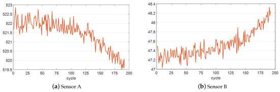
Figure 1.
Sensor measurement data from a piece of equipment.
Consequently, the RUL is difficult to predict in the preliminary state. We presume that the RUL is a constant until it straddles the critical point in the first phase. While in the second phase, we define that RUL is represented by a linear function. Hence, the entire RUL curve is identified as a piece-wise linear function, as shown in Figure 2.
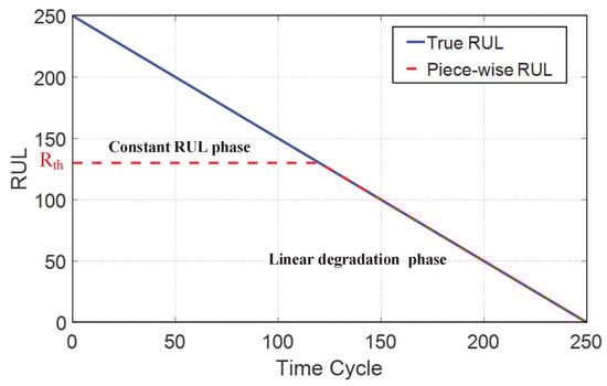
Figure 2.
Piece-wise linear remaining useful life (RUL).
Furthermore, to characterize equipment health condition, there are two methods: physical parameters [45] and stall margins [44]. Physical parameters are usually too complex to obtain. Effectively, stall margins can satisfy the target of better showing the equipment failure state by transforming the sensor measurement data to a one-dimensional HI.
In general, the health indicator , with 0 and 1 corresponding to equipment failure and an intact state, respectively. According to the regularities of RUL distribution regarding the dataset collected, the RUL threshold is ascertained from the predefined critical point . Then, the health indicator of the jth sequence is formulated as
The sensor data and HI of the dataset are processed by polynomial regression. HI estimation at each time-step of the entire dataset is obtained by
where represents dimensional parameters regarding biases and weights. HI trajectories of the dataset are denoted as
where is the HI estimation at the ith time-step of the jth sequence.
3.2. Deep Neural Networks
3.2.1. Convolutional Neural Network
The convolutional neural network (CNN) was proposed by Fukushima [46] and is mainly aimed at pattern recognition and image processing. Indeed, CNNs possess great potential to identify the various prominent patterns of sensor measurement data and extract high-level spatial features.
Normally, the CNN architecture is composed of two types of layers [47]: convolution layers and pooling layers, shown in Figure 3. CNNs are developed to extract abstract features by alternating operations of convolution and pooling [48].
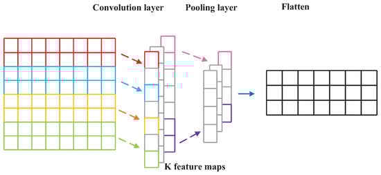
Figure 3.
Convolutional neural network (CNN) architecture.
Convolution layer: In this layer, the previous layer’s feature maps are convolved with convolutional kernels, which are used for feature extraction and feature mapping. Then, the feature map for the next layer is computed through a non-linear function. The output feature maps of the convolution filter are calculated by
where * denotes the convolution operation, l is the lth layer neural network, and and are the input and output of the convolution filter, respectively. is the activation function. is the input of the activation function. and represent weight matrices and additive bias vectors, respectively.
Pooling layers (also known as subsampling layers): In this layer, to reduce the feature map resolution, the output feature maps of the convolution layer are subsampled by proper factors. Average pooling and max pooling are the most common pooling methods. In this paper, the max pooling method is adopted:
where represents the subsample function concerning max pooling.
3.2.2. Recurrent Neural Network and LSTM
A recurrent neural network (RNN) is a natural feed-forward neural network that has been applied successfully owing to its capacity to model highly non-linear data with a sequential nature [49]. A standard RNN is composed of a series of recurrent units to cope with time series problems. The unfold overview of RNN cell architecture is shown in Figure 4. It’s different from the general fully connected neural network, as the output at the current time is also the input of the next time.
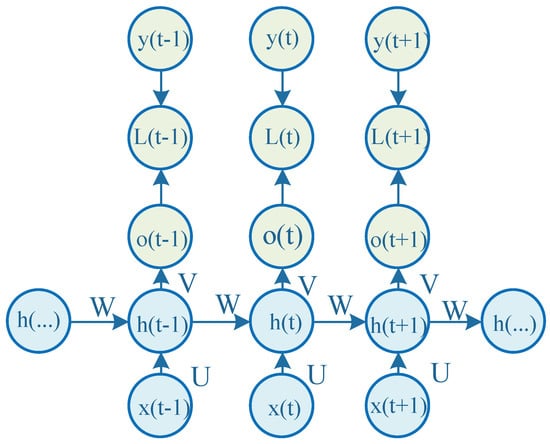
Figure 4.
Recurrent neural network (RNN) cell unfold architecture.
In Figure 4, the same layer weight matrices U, V, and W are re-utilized for each step of computation throughout the sensor data, i.e., weight sharing. is the loss function; is the actual output. The symbol in the parentheses denotes the time-step for the recurrent unit. The RNN cell forward propagation is formulated as follows:
where is the prognostics output of the RNN cell. is the hidden layer. is the element-wise sigmoid activation function. is the element-wise hyperbolic tangent activation function. and are the bias vectors. During the training process, a back-propagation through time (BPTT) algorithm is executed [50]. It is formulated as follows:
However, there will be an accumulation of derivatives of the activation function during backpropagation process. Gradient vanishing or gradient explosion may occur. Hence, improving the RNN cell internal structure is positively efficient.
The LSTM neural network was proposed by Hochreiter and Schmidhuber in 1997 [49]. LSTM is intended to address two special issues that standard RNNs can’t achieve: one issue associated with the standard RNN is the “fading memory”. Once the number of time-steps becomes large, the “future” time-steps will contain virtually no memory of the first inputs as there is no structure in the standard recurrent layer that individually controls the flow of the memory itself. The other issue is that an RNN model is required to confirm the window length in advance, which is formidable to automatically acquire in practical applications [51].
LSTM is a special architecture of RNN. As is shown in Figure 5, the series recurrent unit is the LSTM cell rather than a simple RNN cell. An LSTM cell possesses long-term memory, which is attributable to three gates modulating the flow of information in the LSTM cell: the input gate, forget gate, and output gate.
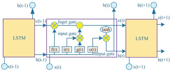
Figure 5.
Long short-term memory (LSTM) cell architecture.
Input gate : It controls what information will be passed to the memory cell based on previous output and current sensor measurement data.
Forget gate : It controls how the memory cell will be updated.
Output gate : It controls which information will be carried to next time-step.
The LSTM forward propagation algorithm is given by Algorithm 1.
| Algorithm 1 LSTM forward propagation algorithm |
|
3.3. Hybrid Scheme
Inspired by prior investigations, CNNs can expand spatially and LSTM can expand in long-term temporary memory. If there are high-frequency sensor measurements or various sensors involved, it is superior to add a convolutional neural network layer before the LSTM layer. Convolution layers are interspersed with pooling layers to reduce computation time and to gradually build up further spatial and configural invariance. LSTM can discover long-term temporary dependency features. The fully connected neural network is good at mapping, and the hybrid DNN will eventually learn an excellent regression model to predict equipment RUL. The proposed scheme is shown in Figure 6. The objective of the proposed scheme is to feed the raw sensor data after feature extracting and nonlinear regression by multilayer networks, then the equipment RUL is obtained.
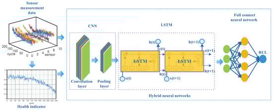
Figure 6.
Hybrid neural networks for RUL prognostics.
We utilize a one-layer convolutional neural network that is composed of one convolution layer and one pooling layer. Meanwhile, we utilize two LSTM layers. For the fully connected neural network, we utilize a multilayer perceptron, which consists of two hidden layers and 50 neurons included in every hidden layer. The mean square error (MSE) is used as the cost function.
where and are the prediction value and true RUL, respectively. N is the total number of samples in the testing set. The Adam optimizer (shown in Algorithm 2), an adaptive learning rate optimization algorithm [52], is employed to train the model.
| Algorithm 2 Adam optimizer algorithm |
|
3.4. Data Preparation
3.4.1. Variance Threshold
The measure data is complex and multidimensional. Features with low variance are convergent, i.e., features are not obviously distinguishable during a sequence, they are ineffective against prognostics performance [53]. Features with a dataset variance lower than will be removed. It is formulated as
where m is the sample size and represents the mean of the feature.
3.4.2. Normalization
Sensor data value scales may be diversiform. To accelerate the convergence rate, we need to normalize the process with respect to each sensor before utilizing data. Two main data normalization methods are exploited widely [54]: z-score normalization (Equation (19)) and min–max normalization (Equation (20)). Specifically, the z-score normalization method makes the sensor data follow the normal distribution, and the min–max normalization method makes the sensor data scale within the range of .
where , , and are the standard deviation, maximum, and minimum with respect to each sensor, respectively.
3.5. Metrics
For the sake of evaluating the performance of the proposed scheme, some evaluation metrics of prediction performance are adopted. These are root mean square error (RMSE), mean absolute percentage error (MAPE), mean absolute error (MAE), and penalty score function. The first four metrics adopted are popularly applied in prognostics tasks. Dissimilarly, the penalty score function is given by PHM2008 competition [44] specifically for RUL prognostics evaluation. The penalty score function is asymmetric, as early prediction is preferred over late prediction. It can be seen from Figure 7 that the tolerance of advanced prognostics is greater than delayed prognostics for the same penalty score value. Evaluation metrics are formulated as follows:
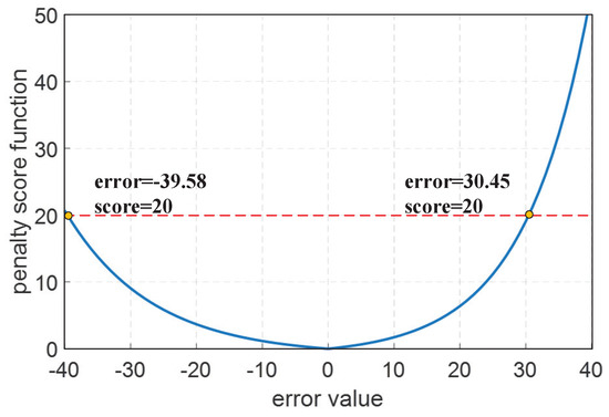
Figure 7.
Penalty score function.
4. Implementation
The flowchart of the proposed scheme of RUL prognostics is presented in Figure 8. Firstly, the raw C-MAPSS dataset is processed to select proper input data using the variance threshold, and the corresponding data are normalized by the z-score normalization method. Next, the preselected data are transformed into a one-dimensional health indicator. The processed datasets are split into the training set and the testing set.
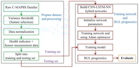
Figure 8.
Flowchart of the proposed scheme.
Furthermore, the CNN-LSTM-NN hybrid networks to be built. Then the network parameters are initialized, which includes the number of hidden layers, the number of neurons, batch size, and so forth. The hybrid scheme takes the training set as the input, and the true RUL of the training set are used as the target outputs. The Adam optimizer is utilized to optimize the training network, with the learning rate set at 0.001 to achieve stable convergence. The number of training epochs is 500. The batch-size is set as 250.
Finally, the testing set is input to the training model for the RUL prognostics, and the evaluation values are obtained.
5. Experiments
In this section, we present our experimental setup, which includes the detailed dataset values and a brief introduction of various prognostics models. To empirically evaluate the effectiveness of the proposed method in addressing equipment RUL prognostics, we conducted a series of experiments on the dataset and compared it with several existing methods. First, we introduce the C-MAPSS dataset. Then we discuss the experimental results along with the analysis.
5.1. C-MAPSS Dataset
The dataset used to verify the proposed model is from NASA [44]. The NASA Commercial Modular Aero-Propulsion System Simulation(C-MAPSS) dataset of turbofan engine degradation simulations is a widely used benchmark dataset [12]. The dataset consists of multiple multivariate time series (shown in Table 1).

Table 1.
Information on the C-MAPSS dataset.
The dataset is supposed to be from the same type of fleet engines. Each engine starts with a different state of initial wear and manufacturing variation, which is unrevealed to the researchers. This wear and variation are considered normal, i.e., they are not considered a fault condition. Three operational settings are given in the dataset. However, we only consider the effect of sensor measurement data in this paper. The measurement data is polluted by sensor noise.
The engine is normally running at the beginning of each time series, and a fault occurs at some point during the series. For the training set, the fault grows in magnitude until system malfunction occurs. For the testing set, the time series ends some time before system failure. The purpose is to prognosticate the numbers of remaining operational cycles before failure in the testing set, i.e., the number of operational cycles after the last cycle in which the engine will continue to run normally. In addition, true RUL values for the testing set data are given.
The dataset contains 4 sub-datasets with different numbers of time series, shown in Table 1. Moreover, the dataset consists of training sets and testing sets. Each row in the data is a snapshot of data taken during a single running time cycle and includes 26 columns: the 1st column indicates the engine ID, the 2nd column indicates the current running cycle number, the 3rd–5th columns indicate three operational settings, the 6th–26th column indicate 21 sensor measurement data that have a substantial effect on engine performance. A detailed description of the dataset can be found in [44].
5.2. Results
In order to empirically evaluate the availability of the proposed scheme for RUL prognostics, the proposed scheme was tested with the testing set. As shown in Figure 9, four testing trajectories selected from four sub-datasets are taken as examples. Though some obvious errors exist between the prediction values and the true RUL values, the prognostic performance is good, especially when the equipment is close to failure. Preferably, accurate RUL prognostics of the equipment in the late phase would be able to improve management availability and reduce maintenance costs because it is extremely necessary to maintain or exchange equipment in the last phase of its lifetime.
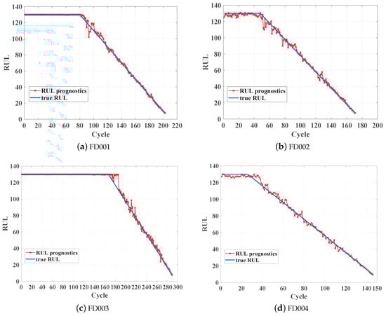
Figure 9.
Model comparison.
To further demonstrate the performance improvement of the proposed scheme, we compared four existing models with the same dataset:
Model 1: Multilayer perceptron (MLP). MLP is a multilayer neural network to address the regression problem. In this paper, the MLP is constructed by using two hidden layers, where each layer consists of 50 neurons. The Relu function is the activation function in each hidden layer.
Model 2: Support vector regression (SVR). SVR is a machine learning method for time series prognostics. The aim of SVR is based on the computation of a linear regression function in a high-dimensional feature space where the input data are mapped via a nonlinear function [55]. In this paper, the Gaussian radical basis function (RBF) is considered as the kernel function.
Model 3: Convolutional neural network. The standard convolutional neural network is introduced in Section 3.2.1. In this paper, we adopt CNN to extract spatial features and the fully connected neural network to obtain a regression model [33].
Model 4: LSTM neural network. The standard LSTM neural network is introduced in Section 3.2.2. In this paper, we adopt two LSTM layers to extract long-term temporary dependencies and the fully connected neural network to achieve RUL prognostics [8].
All of these methods were simulated and applied to the C-MAPSS dataset. Table 2 and Table 3 show the results of the performance comparison using four sub-datasets. Figure 10 shows the model comparison in terms of the RMSE, MAP, MAE, and the average penalty score for the entire testing set. The average penalty score is defined as follows:
where is penalty score function, which is defined in Section 3.5, and N is the sample number of the testing set.
Table 2.
Comparison of performance on sub-dataset (FD001) and sub-dataset (FD002).
Table 3.
Comparison of performance on sub-dataset (FD003) and sub-dataset (FD004).
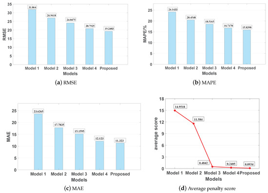
Figure 10.
Model evaluation.
It is evident from Table 2 and Table 3 and Figure 10 that the accuracy of the proposed scheme is higher than that of the MLP, SVM, CNN, and LSTM in adopted metrics defined in Section 3.5. Particularly, the RMSE values of MLP and SVM are 31.864 and 26.9618, respectively. The RMSE value of the proposed scheme is lower by 4.8072 and 1.5522 compared to the CNN and LSTM models, respectively. Moreover, the MAP values of the MLP and SVM are 24.1433% and 20.4548%, respectively. The MAP value of the proposed scheme is lower by 2.6775% and 0.878% compared to the CNN and LSTM models, respectively. The MAE values of MLP and SVM are 23.6265 and 17.7835, respectively. The MAE value of the proposed scheme is lower by 3.8365 and 0.8 compared to the CNN and LSTM models, respectively. In Figure 10, the average penalty scores for the MLP and SVM are much larger than those of the CNN, LSTM, and the proposed scheme as the automatic feature extraction ability of deep learning methods contributes to a higher prediction accuracy than in traditional data-driven methods. Furthermore, the proposed scheme is slightly better than the CNN and LSTM since the addition of the HI and the hybrid DNN structure extracts high-level spatial features and long-term temporal dependency features. In conclusion, the proposed scheme is superior to other models in prediction accuracy and that is encouraging for RUL prognostics tasks.
6. Conclusions
An accurate and reliable RUL prognostic is conducive to equipment management and operation security. On account of the fact that sensor measurement data are highly non-linear and polluted by noise, it is a complex issue to be addressed. In this paper, we proposed a hybrid scheme based on an HI and hybrid DNN model to predict equipment RUL. Differing from preceding methods, hybrid DNNs take full advantage of CNN and LSTM. Specifically, CNN is utilized to extract high-level spatial features, and LSTM is used to learn long-term temporary dependencies. Additionally, the fully connected neural network is modeled to achieve a non-linear regression. Meanwhile, HI describes the equipment’s health state, and the preprocessed sensor measurement data are fed into the hybrid DNN, which can further improve the RUL prognostics performance. The proposed scheme was trained on a dataset of equipment degradation from C-MAPSS. The RMSE, MAPE, MAE, and penalty score metrics were adopted to evaluate the models. The simulation results show that the proposed scheme can satisfactorily predict RUL, especially for the late phase close to failure. In contrast to MLP, SVR, CNN, and LSTM models, compared using the same dataset, the proposed scheme possesses higher accuracy and outperforms comparative models. In the field of industrial production lines, aerospace, military, lathe maintenance, computer hardware service, etc., the proposed scheme can contribute to guaranteeing the security of equipment and reduce maintenance costs.
Author Contributions
Z.K. proposed the prognostics scheme and drafted the paper. Y.C. collected the dataset and wrote the paper. Z.X. performed the simulation and optimized the models. H.L. analyzed the results and modified the paper.
Funding
This research was funded by the National Natural Science Foundation of China (NSFC) under grant 61801518 and the Hubei Provincial Natural Science Foundation of China under grant 2017CFB661.
Conflicts of Interest
The authors declare no conflict of interest.
References
- Zhang, J.; Wang, P.; Yan, R.; Gao, R.X. Long short-term memory for machine remaining life prediction. J. Manuf. Syst. 2018, 48, 78–86. [Google Scholar] [CrossRef]
- Li, W.; Jiao, Z.; Du, L.; Fan, W.; Zhu, Y. An indirect RUL prognosis for lithium-ion battery under vibration stress using Elman neural network. Int. J. Hydrogen Energy 2019, 44, 12270–12276. [Google Scholar] [CrossRef]
- Lei, Y.; Zuo, M.J.; He, Z.; Zi, Y. A multidimensional hybrid intelligent method for gear fault diagnosis. Expert Syst. Appl. 2010, 37, 1419–1430. [Google Scholar] [CrossRef]
- Coro, A.; Macareno, L.M.; Aguirrebeitia, J.; López de Lacalle, L.N. A Methodology to Evaluate the Reliability Impact of the Replacement of Welded Components by Additive Manufacturing Spare Parts. Metals 2019, 9, 932. [Google Scholar] [CrossRef]
- Baysal, M.E.; Sümbül, M.O.; Ekicioğlu, E. A total productive maintenance implementation in a manufacturing company operating in insulation sector in Turkey. In Proceedings of the 2015 6th International Conference on Modeling, Simulation, and Applied Optimization (ICMSAO), Istanbul, Turkey, 27–29 May 2015; pp. 1–7. [Google Scholar] [CrossRef]
- Yang, Z.; Bo, J.; Wei, T. A Review of Current Prognostics and Health Management System Related Standards. Chem. Eng. Trans. 2013, 33, 277–282. [Google Scholar] [CrossRef]
- Asmai, S.; Hussin, B.; Mohd Yusof, M.; Shibghatullah, A. Time Series Prediction Techniques for Estimating Remaining Useful Lifetime of Cutting Tool Failure. Int. Rev. Comput. Softw. 2014, 9, 1783–1790. [Google Scholar] [CrossRef]
- Zheng, S.; Ristovski, K.; Farahat, A.; Gupta, C. Long Short-Term Memory Network for Remaining Useful Life estimation. In Proceedings of the 2017 IEEE International Conference on Prognostics and Health Management (ICPHM), Dallas, TX, USA, 19–21 June 2017; pp. 88–95. [Google Scholar] [CrossRef]
- Liao, L.; Köttig, F. A hybrid framework combining data-driven and model-based methods for system remaining useful life prediction. Appl. Soft Comput. 2016, 44, 191–199. [Google Scholar] [CrossRef]
- Hu, C.; Pei, H.; Wang, Z.; Si, X.; Zhang, Z. A new remaining useful life estimation method for equipment subjected to intervention of imperfect maintenance activities. Chin. J. Aeronaut. 2018, 31, 514–528. [Google Scholar] [CrossRef]
- Okoh, C.; Roy, R.; Mehnen, J.; Redding, L. Overview of Remaining Useful Life Prediction Techniques in Through-life Engineering Services. Procedia CIRP 2014, 16, 158–163. [Google Scholar] [CrossRef]
- Si, X.S.; Wang, W.; Hu, C.H.; Zhou, D.H. Remaining useful life estimation—A review on the statistical data driven approaches. Eur. J. Oper. Res. 2011, 213, 1–14. [Google Scholar] [CrossRef]
- Lei, Y.; Li, N.; Guo, L.; Li, N.; Yan, T.; Lin, J. Machinery health prognostics: A systematic review from data acquisition to RUL prediction. Mech. Syst. Signal Process. 2018, 104, 799–834. [Google Scholar] [CrossRef]
- Basak, S.; Sengupta, S.; Dubey, A. A Data-driven Prognostic Architecture for Online Monitoring of Hard Disks Using Deep LSTM Networks. arXiv 2018, arXiv:1810.08985. [Google Scholar]
- Liu, L.; Guo, Q.; Liu, D.; Peng, Y. Data-Driven Remaining Useful Life Prediction Considering Sensor Anomaly Detection and Data Recovery. IEEE Access 2019, 7, 58336–58345. [Google Scholar] [CrossRef]
- Srivastava, A.N.; Han, J. Machine Learn Ing and Knowledge Discovery for Engineering Systems Health Management; CRC Press: Boca Raton, FL, USA, 2011. [Google Scholar]
- López de Lacalle, L.; Lamikiz, A.; Sánchez, J.; Salgado, M. Effects of tool deflection in the high-speed milling of inclined surfaces. Int. J. Adv. Manuf. Technol. 2004, 24, 621–631. [Google Scholar] [CrossRef]
- Lateef Al-Abdullah, K.I.A.; Abdi, H.; Lim, C.P.; Yassin, W.A. Force and temperature modelling of bone milling using artificial neural networks. Measurement 2018, 116, 25–37. [Google Scholar] [CrossRef]
- Wu, W.; Hu, J.; Zhang, J. Prognostics of Machine Health Condition using an Improved ARIMA-based Prediction method. In Proceedings of the 2007 2nd IEEE Conference on Industrial Electronics and Applications, Harbin, China, 23–25 May 2007; pp. 1062–1067. [Google Scholar] [CrossRef]
- Wang, L.; Zou, H.; Su, J.; Li, L.; Chaudhry, S. An ARIMA-ANN Hybrid Model for Time Series Forecasting. Syst. Res. Behav. Sci. 2013, 30, 244–259. [Google Scholar] [CrossRef]
- Kumar, A.; Chinnam, R.B.; Tseng, F. An HMM and polynomial regression based approach for remaining useful life and health state estimation of cutting tools. Comput. Ind. Eng. 2019, 128, 1008–1014. [Google Scholar] [CrossRef]
- Galagedarage Don, M.; Khan, F. Process Fault Prognosis Using Hidden Markov Model–Bayesian Networks Hybrid Model. Ind. Eng. Chem. Res. 2019, 58, 12041–12053. [Google Scholar] [CrossRef]
- Tobon-Mejia, D.A.; Medjaher, K.; Zerhouni, N.; Tripot, G. A Data-Driven Failure Prognostics Method Based on Mixture of Gaussians Hidden Markov Models. IEEE Trans. Reliab. 2012, 61, 491–503. [Google Scholar] [CrossRef]
- Pang, B.; Feng, W.; Zhao, H.; Li, W.; Chen, S. Research on Modeling Method of Life Prediction for Satellite Lithium Battery Based on SVR. In Proceedings of the 2018 Prognostics and System Health Management Conference (PHM-Chongqing), Chongqing, China, 26–28 October 2018; pp. 1004–1009. [Google Scholar] [CrossRef]
- Das Chagas Moura, M.; Zio, E.; Lins, I.D.; Droguett, E. Failure and reliability prediction by support vector machines regression of time series data. Reliab. Eng. Syst. Saf. 2011, 96, 1527–1534. [Google Scholar] [CrossRef]
- Benkedjouh, T.; Medjaher, K.; Zerhouni, N.; Rechak, S. Remaining useful life estimation based on nonlinear feature reduction and support vector regression. Eng. Appl. Artif. Intell. 2013, 26, 1751–1760. [Google Scholar] [CrossRef]
- Varanasi, J.; Tripathi, M.M. Artificial Neural Network based wind speed amp; power forecasting in US wind energy farms. In Proceedings of the 2016 IEEE 1st International Conference on Power Electronics, Intelligent Control and Energy Systems (ICPEICES), Delhi, India, 4–6 July 2016; pp. 1–6. [Google Scholar] [CrossRef]
- Arnaiz-González, Á.; Fernández-Valdivielso, A.; Bustillo, A.; López de Lacalle, L.N. Using artificial neural networks for the prediction of dimensional error on inclined surfaces manufactured by ball-end milling. Int. J. Adv. Manuf. Technol. 2016, 83, 847–859. [Google Scholar] [CrossRef]
- Wu, D.; Jennings, C.; Terpenny, J.; Gao, R.; Tirupatikumara, S. A Comparative Study on Machine Learning Algorithms for Smart Manufacturing: Tool Wear Prediction Using Random Forests. J. Manuf. Sci. Eng. Trans. ASME 2017, 139. [Google Scholar] [CrossRef]
- Mandal, D.; Pal, S.K.; Saha, P. Modeling of electrical discharge machining process using back propagation neural network and multi-objective optimization using non-dominating sorting genetic algorithm-II. J. Mater. Process. Technol. 2007, 186, 154–162. [Google Scholar] [CrossRef]
- LeCun, Y.; Bengio, Y.; Hinton, G. Deep learning. Nature 2015, 521, 436. [Google Scholar] [CrossRef] [PubMed]
- Wang, J.; Zhuang, J.; Duan, L.; Cheng, W. A multi-scale convolution neural network for featureless fault diagnosis. In Proceedings of the 2016 International Symposium on Flexible Automation (ISFA), Cleveland, OH, USA, 1–3 August 2016; pp. 65–70. [Google Scholar] [CrossRef]
- Ren, L.; Sun, Y.; Wang, H.; Zhang, L. Prediction of Bearing Remaining Useful Life With Deep Convolution Neural Network. IEEE Access 2018, 6, 13041–13049. [Google Scholar] [CrossRef]
- Sateesh Babu, G.; Zhao, P.; Li, X.L. Deep Convolutional Neural Network Based Regression Approach for Estimation of Remaining Useful Life. In Database Systems for Advanced Applications; Navathe, S.B., Wu, W., Shekhar, S., Du, X., Wang, X.S., Xiong, H., Eds.; Springer: Cham, Switzerland, 2016; pp. 214–228. [Google Scholar]
- Zhang, J.; Wang, J.; He, L.; Li, Z.; Yu, P.S. Layerwise Perturbation-Based Adversarial Training for Hard Drive Health Degree Prediction. In Proceedings of the 2018 IEEE International Conference on Data Mining (ICDM), Singapore, 17–20 November 2018; pp. 1428–1433. [Google Scholar] [CrossRef]
- Guo, L.; Li, N.; Jia, F.; Lei, Y.; Lin, J. A Recurrent Neural Network Based Health Indicator for Remaining Useful Life Prediction of Bearings. Neurocomputing 2017, 240, 98–109. [Google Scholar] [CrossRef]
- Wang, J.; Yu, L.C.; Lai, K.R.; Zhang, X.J. Dimensional Sentiment Analysis Using a Regional CNN-LSTM Model. In Proceedings of the 54th Annual Meeting of the Association for Computational Linguistics, Berlin, Germany, 7–12 August 2016; pp. 225–230. [Google Scholar] [CrossRef]
- Sainath, T.N.; Vinyals, O.; Senior, A.; Sak, H. Convolutional, Long Short-Term Memory, fully connected Deep Neural Networks. In Proceedings of the 2015 IEEE International Conference on Acoustics, Speech and Signal Processing (ICASSP), Brisbane, Australia, 19–24 April 2015; pp. 4580–4584. [Google Scholar] [CrossRef]
- Ullah, A.; Ahmad, J.; Muhammad, K.; Sajjad, M.; Baik, S.W. Action Recognition in Video Sequences using Deep Bi-Directional LSTM With CNN Features. IEEE Access 2018, 6, 1155–1166. [Google Scholar] [CrossRef]
- Oh, S.L.; Ng, E.Y.; Tan, R.S.; Acharya, U.R. Automated diagnosis of arrhythmia using combination of CNN and LSTM techniques with variable length heart beats. Comput. Biol. Med. 2018, 102, 278–287. [Google Scholar] [CrossRef]
- Zhao, R.; Yan, R.; Wang, J.; Mao, K. Learning to Monitor Machine Health with Convolutional Bi-Directional LSTM Networks. Sensors 2017, 17, 273. [Google Scholar] [CrossRef]
- Yue, G.; Ping, G.; Lanxin, L. An End-to-End model based on CNN-LSTM for Industrial Fault Diagnosis and Prognosis. In Proceedings of the 2018 International Conference on Network Infrastructure and Digital Content (IC-NIDC), Guiyang, China, 22–24 August 2018; pp. 274–278. [Google Scholar] [CrossRef]
- Kim, T.Y.; Cho, S.B. Predicting residential energy consumption using CNN-LSTM neural networks. Energy 2019, 182, 72–81. [Google Scholar] [CrossRef]
- Saxena, A.; Goebel, K.; Simon, D.; Eklund, N. Damage propagation modeling for aircraft engine run-to-failure simulation. In Proceedings of the 2008 International Conference on Prognostics and Health Management, Denver, CO, USA, 6–9 October 2008; pp. 1–9. [Google Scholar] [CrossRef]
- Volponi, A.J.; DePold, H.; Ganguli, R.; Daguang, C. The Use of Kalman Filter and Neural Network Methodologies in Gas Turbine Performance Diagnostics: A Comparative Study. J. Eng. Gas Turbines Power 2003, 125. [Google Scholar] [CrossRef]
- Fukushima, K. Neocognitron: A self-organizing neural network model for a mechanism of pattern recognition unaffected by shift in position. Biol. Cybern. 1980, 36, 193–202. [Google Scholar] [CrossRef] [PubMed]
- Chen, Z.; Li, C.; Sanchez, R. Gearbox Fault Identification and Classification with Convolutional Neural Networks. Shock Vib. 2015. [Google Scholar] [CrossRef]
- Rhanoui, M.; Mikram, M.; Yousfi, S.; Barzali, S. A CNN-BiLSTM Model for Document-Level Sentiment Analysis. Mach. Learn. Knowl. Extr. 2019, 1, 832–847. [Google Scholar] [CrossRef]
- Hochreiter, S.; Schmidhuber, J. Long Short-Term Memory. Neural Comput. 1997, 9, 1735–1780. [Google Scholar] [CrossRef]
- Hwan Lee, J.; Kim, H. Empirical Investigation of Stale Value Tolerance on Parallel RNN Training. In Proceedings of the 2019 IEEE International Symposium on Performance Analysis of Systems and Software (ISPASS), Madison, WI, USA, 24–26 March 2019; pp. 153–164. [Google Scholar] [CrossRef]
- Ma, X.; Tao, Z.; Wang, Y.; Yu, H.; Wang, Y. Long short-term memory neural network for traffic speed prediction using remote microwave sensor data. Transp. Res. Part C Emerg. Technol. 2015, 54, 187–197. [Google Scholar] [CrossRef]
- Chang, Z.; Zhang, Y.; Chen, W. Effective Adam-Optimized LSTM Neural Network for Electricity Price Forecasting. In Proceedings of the 2018 IEEE 9th International Conference on Software Engineering and Service Science (ICSESS), Beijing, China, 23–25 November 2018; pp. 245–248. [Google Scholar] [CrossRef]
- Guan, Y.; Dy, J.G.; Jordan, M.I. A Unified Probabilistic Model for Global and Local Unsupervised Feature Selection. In Proceedings of the 28th International Conference on Machine Learning (ICML), Bellevue, WA, USA, 28 June–2 July 2011; pp. 1073–1080. [Google Scholar]
- Patro, S.G.K.; Sahu, K.K. Normalization: A Preprocessing Stage. arXiv 2015, arXiv:1503.06462. [Google Scholar] [CrossRef]
- Basak, D.; Pal, S.; Patranabis, D.C. Support vector regression. Neural Inf. Process. Lett. Rev. 2007, 11, 203–224. [Google Scholar]


© 2019 by the authors. Licensee MDPI, Basel, Switzerland. This article is an open access article distributed under the terms and conditions of the Creative Commons Attribution (CC BY) license (http://creativecommons.org/licenses/by/4.0/).