Labeling Confidence Values for Wafer-Handling Robot Arm Performance Using a Feature-Based General Regression Neural Network and Genetic Algorithm

Abstract

The prognosis and management of machine health statuses are emerging research topics. In this study, the performance degradation of a wafer-handling robot arm (WHRA) was predicted using the proposed machine-learning approach. This method considers the eccentric vertical and planar position deviations from a wafer mark using a charge-coupled device (CCD) camera. Synthesized position signals were defined using the square root of x- and y-axes deviations in the horizontal view and the square of the wafer mark diameter in the vertical view. A feature extraction method was used to determine the position status on the basis of these displacements and the area of a wafer mark in a CCD image. The root mean square error and mean, maximum, and minimum of the synthesized position signals were extracted through feature extraction and used for data mining by a general regression neural network (GRNN) and logistic regression (LR) models. The lifetime assessment by confidence value of the WHRA’s remaining useful life (RUL) by the genetic algorithm/GRNN exhibited nearly the same trend as that predicted through a run-to-failure LR model. The experimental results indicated that the proposed methodology can be used for proactive assessments of the RUL of WHRAs.

1. Introduction

In a semiconductor production factory, a module of equipment that has malfunctioned or shut down must generally be repaired or replaced with a new module within the shop floor system. This activity results in equipment downtime and considerable maintenance costs, which, in turn, yield loss of production profit. In most processes, a wafer-handling robot arm (WHRA) is used to transfer wafers between the cassette and the chamber. However, a deviation in WHRA positioning may result in wafer fragmentation or backward positioning in processes such as in spin coating and yellow light generation. Although machine manufacturers have provided a solution, i.e., position compensation of robot arms, in the latest generation of machines, manufacturing engineers have attempted to upgrade old machines by implementing new controller boards. However, because of the additional cost this method incurs, users are resistant to such upgrade techniques. Therefore, an effective method for predicting maintenance time and a reliable kit for adding a positioning inspection module to existing equipment are required [1].

Conventional maintenance involves breakdown maintenance, scheduled preventive maintenance, and condition-based maintenance (CBM). In CBM, experts monitor a sensorless machine’s health based on data, such as the driving voltage or current, obtained by attaching sensors, such as accelerometers and microphones, at key positions or locations with well-known domain-knowledge on the machine. In previous studies [2,3,4], some systematic, data-driven methods were used to trace the cause of major problems occurring in the ball screw of a feed drive system or Computer Numerical Control (CNC) machine in a manufacturing process. In that research, the failure signature was identified and classified using various prediction models. With trends such as big data, the Internet of Things, and smart manufacturing, smart analytics can determine the health statuses of CNC machines. The acquisition of large volumes of sensor data and data-driven approaches have developed in recent machine-learning research. Data cleaning and feature engineering are required for fast computing for effective machinery prognostics. Current methods to predict the failure of rotating machinery through CBM are based on physics-based or data-driven prognostics models. These methods are classified as conventional reliability models, condition-based prognostics models, or those integrating reliability and prognostics models [5].

A proactive reliability assessment method for a WHRA was studied in [1]; predictions were based on a sample degradation trend obtained through the Wiener stochastic process and random sampling with controlled uncertainty using a Monte Carlo simulation. The study’s aim was to create a prognostic and health management model for predicting the lifetime and monitoring the state of the WHRA prior to maintenance. The reliability of an individual unit or subsystem during shop floor use is vital to the maintenance of the life of the unit or system. The remaining useful life (RUL) indicates the ability of a unit or system to survive in the future. When operation degrades, it is essential to estimate the RUL accuracy in order to make the appropriate decision for failure prevention. In [6], the prediction of the RUL of a bearing test rig was performed on the basis of a hazard model and logistic regression (LR) model by considering hard failure and multiple degradation features. Furthermore, a systematic methodology for the prognosis, health assessment, and RUL of ball screws was proposed in [7]. Because the RUL cannot be assumed to degrade linearly with the progress of the work cycle, RUL profiles may initially be constant before degrading according to a certain mathematical function at a certain inflection point until the final failure occurs. Considering the entire history of a working asset until its failure would restrict the RUL model, as partial maintenance procedures will result in the asset exhibiting an improved health condition, and so only minimal repair is induced. The initial conditions of physical systems are usually unknown due to manufacturing deficiencies, the replacements of parts of the system, and imperfect maintenance [8].

A LR model is usually adopted to relate the probability of an event to a set of covariates, and can be utilized in degradation analyses [6,9]. This process requires information on degradation features and the relationship between the output of the reliability function and the estimated model parameters. Nevertheless, the LR method can be used to determine the RUL of a machine [5] or predict component failure [8]. Such RUL learning curves are based on the supervision of the machine status. Such supervised health and degradation requires an index for labeling the working asset status; for example, for a cutting tool, a value of 1 denotes initial healthy status, whereas 0 denotes failure, such as through tool flute which affects the surface roughness due to poor cutting performance. During a tool’s operational lifetime, the value decreases with the remaining life, and calls for maintenance may be made after the index reaches a certain value, such as 0.3, depending on the type of CBM. However, run-to-failure maintenance is time consuming and requires that a considerable number of test experiments be conducted. The labeling of machine health from 1 to 0 is usually unknown in advance, and the decisive value, for example 0.3, for calling for maintenance is subjective.

In practice, the probability of calling for WHRA maintenance after falling into damage status is high, due to errors such as misalignment of the wafer position when transferring the wafer to the cassette, mismatch of the robot’s belt gear engagement, and unexpected power shutdowns. Therefore, developing a method of prognosis for WHRA performance degradation and health management is an emerging field of study. However, the confidence values of 1 to 0 are estimated in the first stage of the RUL model’s construction. The following sections present the merits of a general regression neural network (GRNN) to manipulate the supervised learning of an unknown label based on feature extraction. Additionally, LR, considering 1 as the label for initial healthy status and 0 as the call-for-maintenance label based on experimental data, is presented. The feature-based genetic algorithm (GA)–GRNN model is shown to predict the same trend as a conventional run-to-failure maintenance LR model on the basis of the same input features in the GRNN.

2 Method

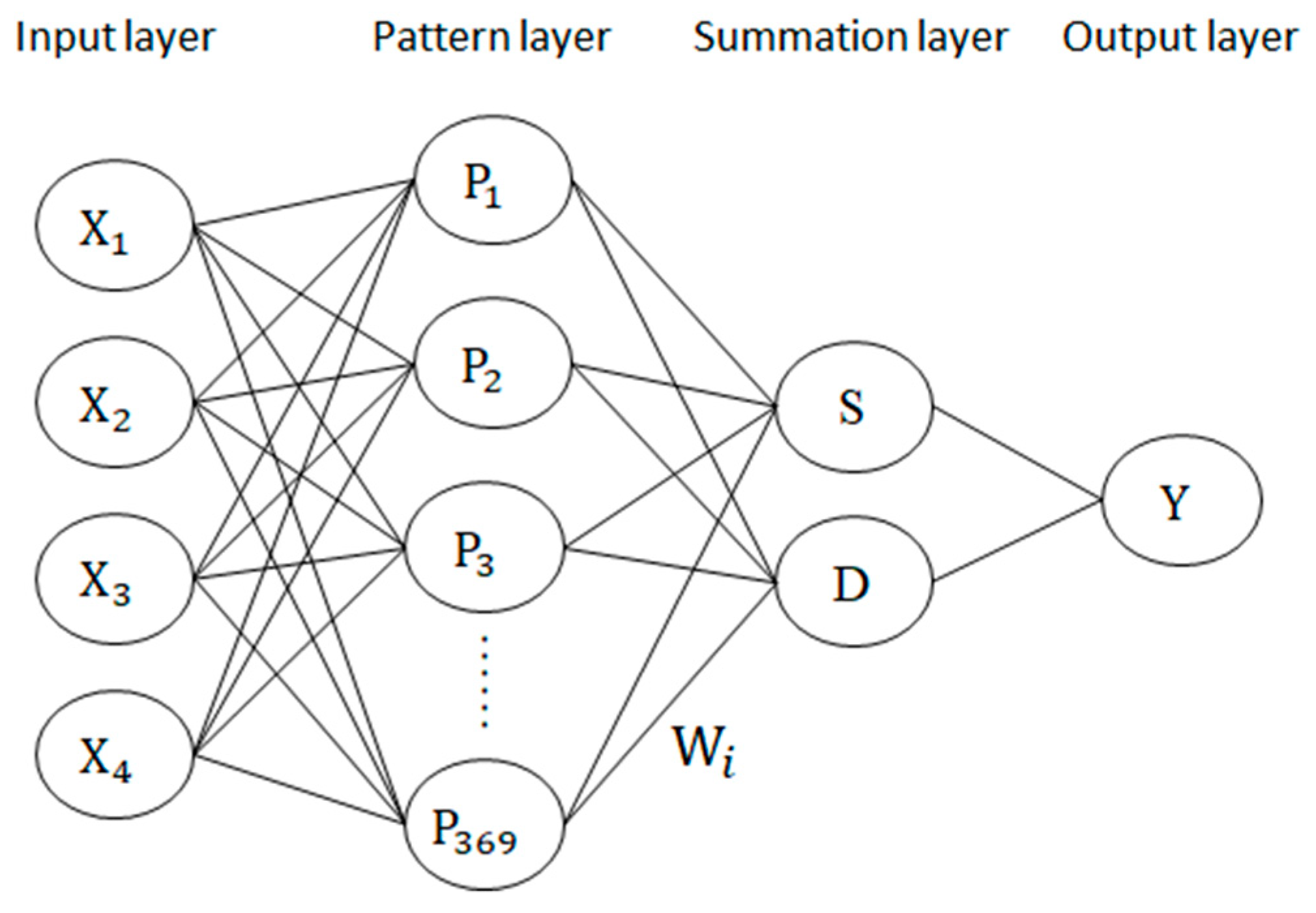
2.1. General Regression Neural Network

A GRNN is a type of neural network based on nonlinear regression. It is established using a one-pass learning algorithm with a highly parallel structure, which was proposed by Specht in 1991 [10].

As illustrated in Figure 1, the GRNN structure consists of four layers: the input layer, pattern layer, summation layer, and output layer. The number of inputs for the network is equal to the number of independent features (n) in the vector X = [x_1, x_2, ..., x_n], which denotes a single input observation. The number of neurons (k) in the pattern layer is equal to the number of data sets used for training, and each neuron contains an input X. Equation (1) represents the Euclidean distance between the input and each neuron in the pattern layer. The symbols σ, b and $W_i$ in Equations (2) and (3) stand for spread parameter, bias, and the weight of each neuron in the pattern layer, respectively. The value of the spread parameter behaves like a regression action during network modeling, and will influence the predictive result greatly. The larger the value of σ, the smoother output curve of the forecast outcome. By adjusting parameters σ and b, the output of each neuron in the pattern layer can be obtained. The summation layer of the GRNN in this study consists of only two neurons: the S- and D-summation neurons. The number of S-summation layers is equal to the number of the neuron of the output layer. It is packaged by the predicted CV from the pattern layer and manipulated by Equation (3). The number of the D-summation is a single value and stands for one. Only one $y_i$ is the desired output (which is the confidence value (CV) of the machine’s health status [11]) in this study. A GA is used to determine the optimal spread parameters σ and b in the GRNN. The relationship between the two is, in a way, a reciprocal one, as indicated in the exponential term of Equation (2). The final output value obtained as the weighted average is given in Equation (3).

$$D_i^2={(X-P_i)}^T(X-P_i)$$

(1)

$$W_i=\exp (\frac{-D_i^{2}b}{2{\sigma }^2}),0<\mathsf{\sigma },\mathrm{b}<1$$

(2)

$$\mathrm{Y}=\frac{\mathrm{S}}{D}=\frac{{{\displaystyle \sum }}_{i=1}^n{y}_i\exp (\frac{-D_i^2}{2{\sigma }^2})}{{{\displaystyle \sum }}_{i=1}^n\exp (\frac{-D_i^2}{2{\sigma }^2})}$$

(3)

The k-fold cross-validation method is used to segment the training data into modeling data and validation data. The training modeling and validation data are split into k groups, and each GRNN group model is trained at a different time. Further, by adjusting the values of the spread parameter σ and parameter b using the GA, the root mean square error (RMSE) value between the predicted output of the GRNN model and the corresponding output value of the training data are minimized; that is, the optimal σ and b of the GRNN model are obtained. Finally, the output of the entire GRNN model is obtained from the average of the output of the k GRNN models. Figure 2 presents a flow chart for determining the CV of a RUL using the GRNN model with k-fold cross-validation and GA optimization.

2.2. LR Model

In Equation (4), the sigmoid function is used for predicting the output of LR with the inputs features $x_1–x_n$ in Equation (5) using model parameters ${\theta }_0–{\theta }_n$. A conventional run-to-failure LR sets y as a constant to 1 for the initial healthy status, to 0 for failure, and to 0–1 for the rest of the work asset’s lifetime. To build the RUL model accurately with a LR, the difference between the predicted $h_{\theta }(x)$ and $y$ is minimized. Therefore, one trains the model parameters for each ${\theta }_0–{\theta }_n$ based on Equation (4) to predict actual the CV, y, of the machine’s health. The model parameters for ${\theta }_0$–${\theta }_n$ can be derived using the Bernoulli distribution, maximum likelihood estimation (MLE), a loss function, and the method of gradient descent.

$$h_{\theta }(x)=\frac{1}{1+e^{-{\theta }^{T}x}}$$

(4)

$${\theta }^{T}x={\theta }_0+{\theta }_1{x}_1+{\theta }_2{x}_2+{\theta }_3{x}_3+\dots +{\theta }_n{x}_n$$

(5)

The probability by Bernoulli distribution is given by Equation (6).

$$p(y|x)=h_{\theta }{(x)}^y{(1-h_{\theta }(x))}^{1-y}=\{\begin{array}{c}{h}_{\theta }(x) if y=1\\ 1-h_{\theta }(x) if y=0\end{array}$$

(6)

The MLE function is applied by multiplying each probability in Equation (6) after the most likely real outputs y are obtained from the inputs $X_1–X_m$ and the model parameters ${\theta }_0–{\theta }_m$. Thus, Equation (7) provides a likelihood estimation function based on m known samples and the loss function in Equation (8). Iterations of the gradient descent method with the learning rate ($\alpha$) to find the value of each model parameter ${\theta }_j$ are performed according to Equations (9) and (10).

$$L(\theta )={\displaystyle \prod }_{i=1}^{m}p(y^{(i)}|x^{(i)};\theta )={\displaystyle \prod }_{i=1}^m{h}_{\theta }{(x^{(i)})}^{y^{(i)}}{(1-h_{\theta }(x^{(i)}))}^{1-y^{(i)}}$$

(7)

$$J(\theta )=-\log L(\theta )={\displaystyle \sum }_{i=1}^m(\log (1+ex{p}^{{\theta }^T{x}^{(i)}})-y^{(i)}{\theta }^T{x}^{(i)})$$

(8)

$$\frac{\partial J(\theta )}{\partial {\theta }_j}=\frac{\partial {{\displaystyle \sum }}_{i=1}^m(\log (1+ex{p}^{{\theta }^T{x}^{(i)}})-y^{(i)}{\theta }^T{x}^{(i)})}{\partial {\theta }_j}={\displaystyle \sum }_{i=1}^m(h_{\theta }(x^{(i)})-y^{(i)})x_j^{(i)}$$

(9)

$${\theta }_j={\theta }_j-\alpha {\displaystyle \sum }_{i=1}^m(h_{\theta }(x^{(i)})-y^{(i)})x_j^{(i)}$$

(10)

3. Application

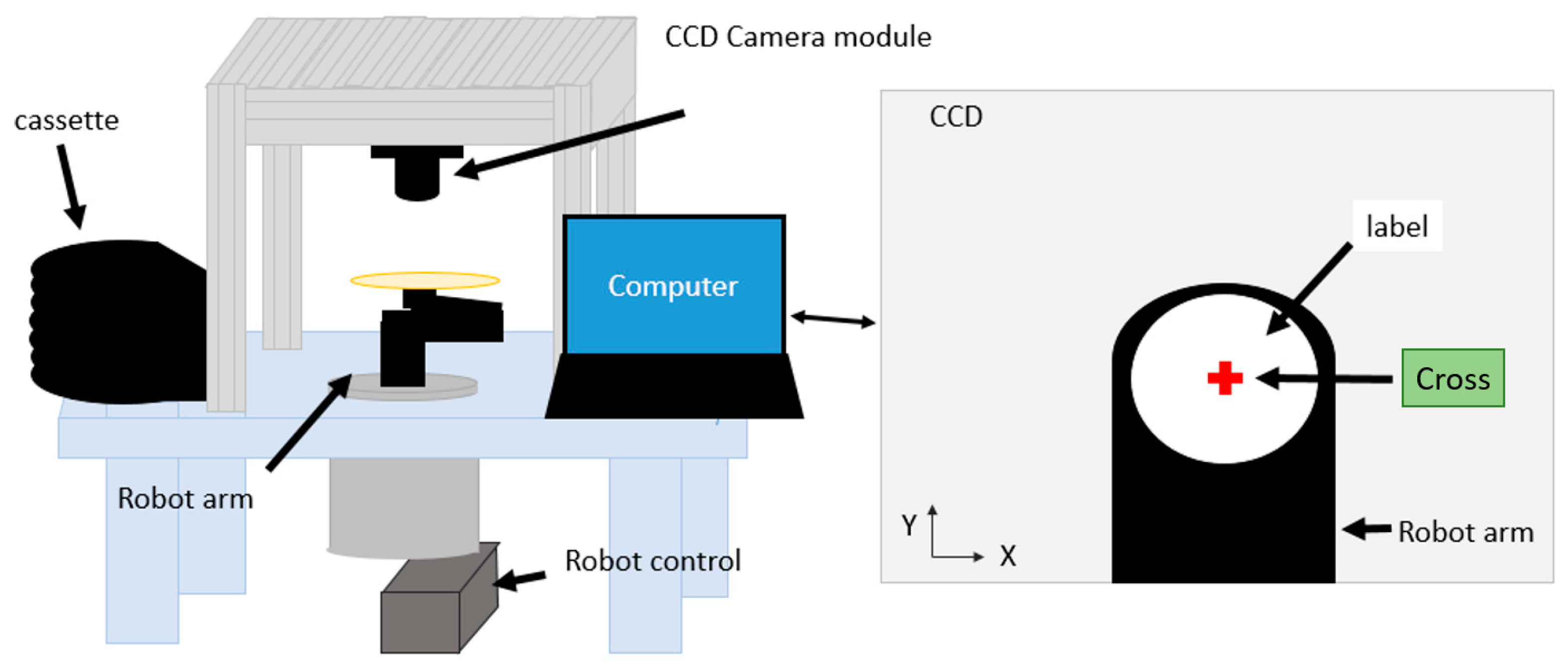
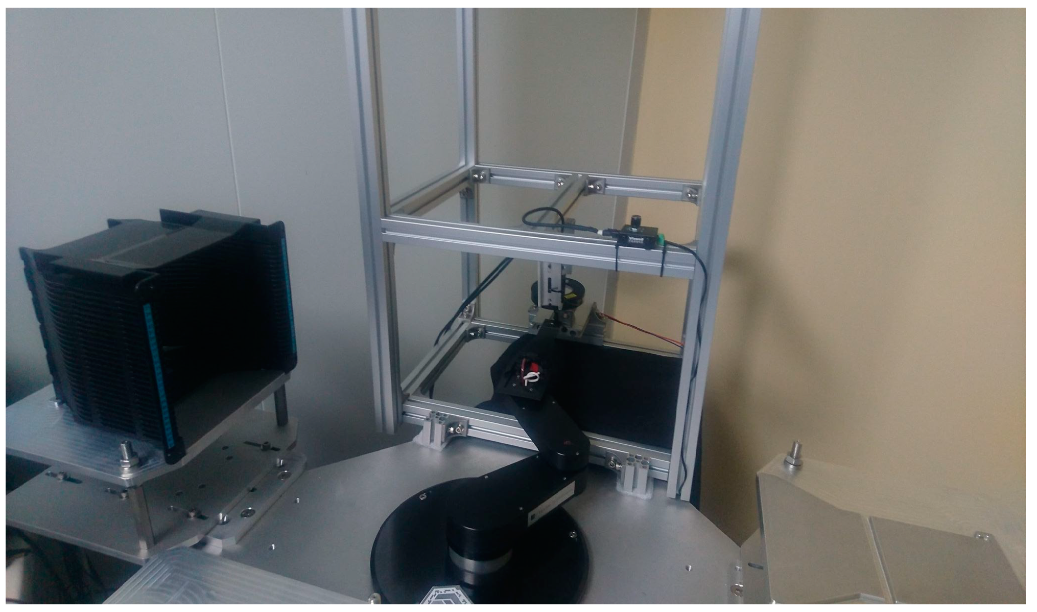
3.1. Experiment Setup and a Call-for-Maintenance Case

An in-lab experiment was performed to construct a plug-in or add-on fixed, charge-coupled device (CCD) camera monitoring system for the inspection of WHRA performance degradation by recording the deviation from the center of the wafer (red cross wafer mark in Figure 3) and measuring the circle peripheral (the white circle in Figure 3) in the vertical view each day. Figure 3 illustrates the vision of CCD. In [1], the potential failure mechanism was the wear of the belt teeth according to the test profiles; thus, this was the cause of an eccentricity problem during wafer transfer. Figure 4 presents a picture of the WHRA, cassette, and CCD camera used in [1]; the same setup was used in this study.

In this experiment, 2,819,678 data were recorded by the CCD camera and categorized as circle radii ${\mathit{C}}_{\mathit{R}}$ or eccentric positions measured along the x-axis (${\mathit{C}}_{\mathit{X}}$) or y-axis (${\mathit{C}}_{\mathit{Y}}$), as presented in Figure 5a with a moving average by 16 points and with original data plot in Figure 5b. Each of these positioning deviations represents a symptom of a problem requiring a call for maintenance. Figure 6 indicates that the synergy-deviated positioning by Equation (11) grows monotonically.

$${\displaystyle \mathit{A}=\sqrt{{\mathit{C}}_{\mathit{X}}{}^2+{\mathit{C}}_{\mathit{Y}}{}^2+{\mathit{C}}_{\mathit{R}}{}^2}}$$

(11)

In this study, the X and Y position deviation and the enlargement of the circle diameter of the CCD constituted an index of the possibility of necessary run-to-failure maintenance during the RUL. Thus, the synergy-deviated position A in Equation (11) is used as a guide for WHRA degradation. The movement cycle of the WHRA from the cassette to the destination, for the CCD’s monitoring, takes approximately 11 s. The positioning data for each of ${\mathit{C}}_{\mathit{X}}$, ${\mathit{C}}_{\mathit{Y}}$, and ${\mathit{C}}_{\mathit{R}}$ were stored as approximately 7800 records per day. Far fewer than 7800 records per day were recorded for 38 days due to possible temporary power shutdowns in the laboratory. The data log for the 38 days was deleted, and the data of 331 days remained for the analysis. Thus, the raw data formed a 331 × 7800 matrix.

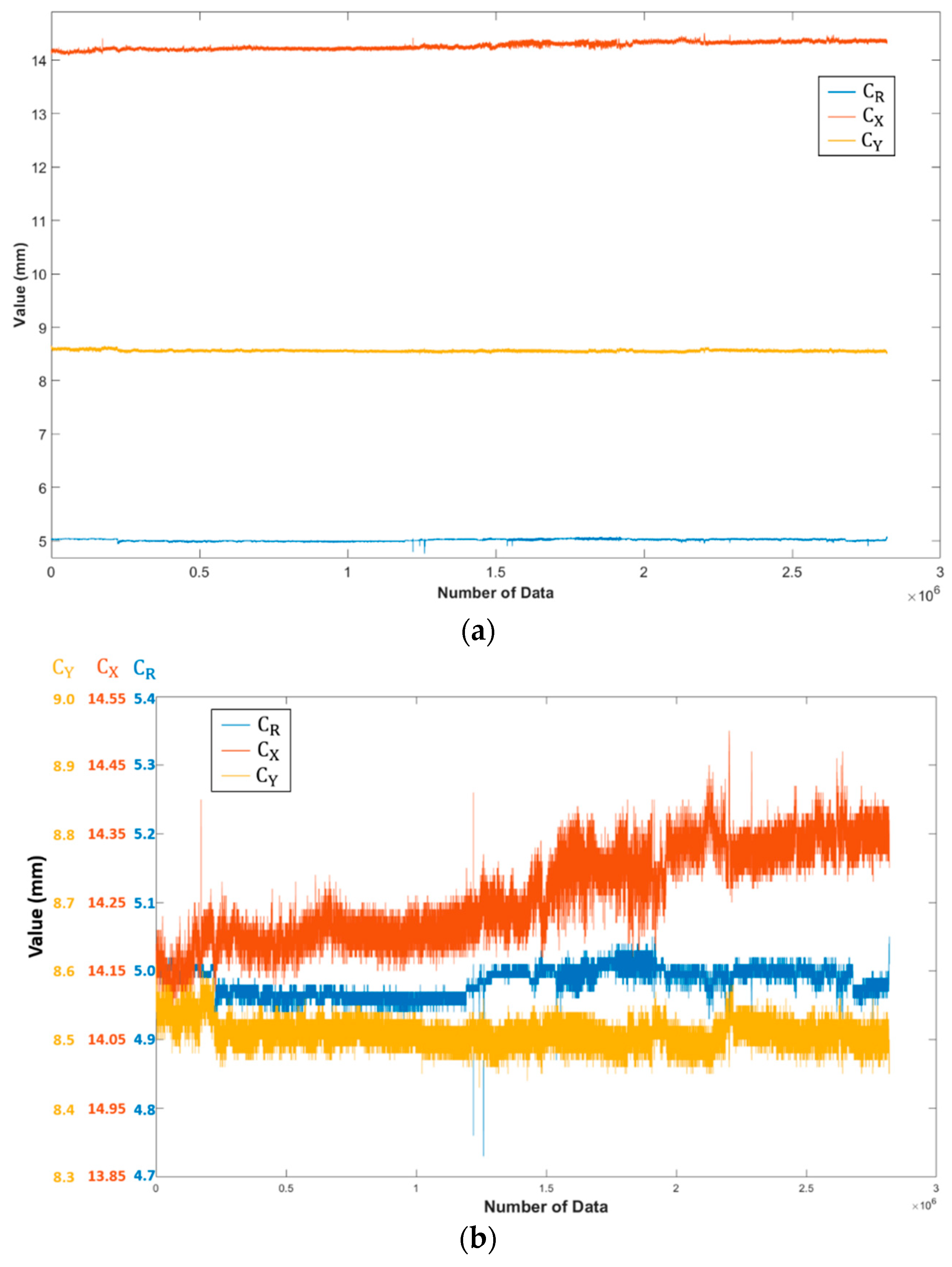
3.2. Data Mining with Feature Extraction

Feature selection helps to avoid overfitting and improve model performance, and provides efficient and cost-effective process monitoring while acquiring better insights into the underlying processes that generated the data [12]. Various time domain features can be extracted to describe the characteristics of the sensed signal from different aspects, such as RMS, kurtosis, and crest factor etc. For example [13], any spikiness in the vibration signals indicated by the crest factor and kurtosis implies incipient defects, where the high energy level given by the value of RMS indicates sever defects. Therefore, selected feature fusion might result in better data mining for machine learning. As displayed in Figure 7, the raw data converted to synergy position signals were divided into 331 segments after packaging, as in Equation (11). Each segment was labeled as one cell with its own feature vectors, and each feature vector contained nine feature elements, namely, the RMS error, kurtosis, variance, crest factor, standard deviation, skewness, mean, maximum, and minimum of the synergy position signals.

Before feature extraction from the nine features of the feature vector of each of the 331 cells, outliers (extreme values) were removed using the Z-score technique. The criterion for determining outliers though Z-score computation was set at three times the standard deviation. A red dot was treated as an outlier after Z-score computation (Figure 8). Therefore, 16 cells were removed from the original 331 cells. The representative quantitative values were extracted from the remaining 315 cells, and reflected the WHRA degradation behavior from health status to failure mode.

Using all the extracted features to assess the prognostic-diagnosis health model is unfeasible and inefficient, since some extracted features have a low contribution in classification models. Therefore, the Fisher criterion was used to select among the nine features those that could distinguish between healthy status class (labeled as CV of 1) and call-for-maintenance class (labeled as CV of 0). The Fisher criterion score (Equation (12)) of each feature was calculated to identify the significant features from the feature vectors as follows:

$$\mathrm{Fisher}\mathrm{score}=\frac{{\mu }_1-{\mu }_2}{S_1{}^2+S_2{}^2}$$

(12)

where μ and $\mathrm{S}$ indicate the mean and standard deviation, respectively, of each class; subscripts 1 and 2 represent classes 1 and 2, respectively. Figure 9 plots the Fisher scores for all nine features. Four high-score features (RMS error, mean, maximum, and minimum of signals) that could distinguish between the healthy and call-for-maintenance classes were selected. For the 315 cells, 315 × 4 arrays were constructed. Each cell contained four column features, including the healthy status class, working asset, and call-for-maintenance class to be used for the next CV labeling. The 315 × 4 arrays were normalized to a N (μ,$\mathrm{S}$) distribution within [0,1]. The formula is given in Equation (13) for the new value of each cell feature:

$$X_{ij}=\frac{x_{ij}-x_{\min }}{x_{\max }-x_{\min }},\mathrm{where}i=1,2,\dots ,315\mathrm{and}j=1,2,3,4.$$

(13)

This normalization was preserved as a new 315 × 4 array, which was then used in the GA–GRNN and LR models of the RUL.

3.3. Labeling the Initial CVs from 1 to 0 as Linearly-Spaced Values for GRNN

The four high-score features, i.e., the RMS error, mean, maximum, and minimum of signals, are treated as the variables of the input layer ${\mathit{X}}_{\mathbf{1}} ~ {\mathit{X}}_{\mathbf{4}}$ in Figure 1, and the initial CVs for ${\mathit{P}}_{\mathbf{1}}–{\mathit{P}}_{\mathbf{315}}$ from 1 to 0 as linearly-spaced values in the pattern layer in Figure 1. An artificial neural network (ANN) is a mathematical model based on biological neural networks, and is trained using previously recorded data. An ANN determines the relationship between the input and output variables through nonlinear regression analysis. For three-fold cross-validation of the GA-GRNN, 315 × 4 data points were divided into three. Two-thirds of the 315 data points were trained, and one-third were tested. Two parameters, σ and b in Equation (2), were tuned by the GA within the GRNN structure. Convergence of the GA based on the other one-third for validation was achieved, and a very low RMS error was obtained. “Best” and “Mean” in Figure 10 indicate the fitness value (convergence) of the optimized particle and the average fitness value of particles, respectively. Both converge at a fitness value of approximately 0.0125 after approximately 30 iterations.

After three GA–GRNN models were built, the data of the original 331 days plus the 38 unexpected power shutdown days were packaged, and the average outputs y are plotted in Figure 11 as black dots. As mentioned before, the initial CVs of the WHRA start from 1 and descend to 0 (denoted by the blue straight line covering 369 days in Figure 11) when the curve of the RUL of the WHRA is unknown in a prior iteration. The entire history of a working WHRA until its failure or call for maintainence would restrict the accuracy of the RUL model, as previous partial maintenance procedures result in the asset exhibiting an improved health condition. Users are keen to determine unclear working lifetimes and health statuses when the WHRA is reused, repaired, and a frequent occurrence in practice.

3.4. Result Discussion

From Day 1, the CV indicating the health status was not equal to 1 when the spread parameter σ was tuned by the GA. Because the GRNN uses probabilistic-based network regression, certain standard deviations were likely to be within the prediction range. Such statistical effects resulted in the manipulation of the CV score by the input layer, resulting in lower weightings despite the initial set (estimate) being labeled 1; this was relayed to a lower CV, for example, 0.73, as shown in Figure 11. However, a high weighting factor from the other nodes rendered from the rest of the pattern layer nodes contributed to the summation layer and resulted in a low predicted output CV. That is, in this study, the predicted GRNN score (CV, y_i) was influenced by the machine degradation, and the CV score was recalculated based on the entire WHRA’s operation history until the call for maintenance. An eight-point moving average of the output CV is plotted as a red curve in Figure 11. Double-flat curves with an inflection (decrease) in their health status due to machine degradation were similar to those obtained by the LR method, as presented in Figure 12. Four high-score features (RMS error, mean, maximum, and minimum of signals) of the call for maintenance are input into LR.

From Figure 12, according to the observations, the machine performance degraded from Days 20–50 and reverted from Days 230–260. Conventional LR models to assess machine run-to-failure performance, for example, adopt the first seven CV = 1 and last seven CV = 0 cells. The other CVs used to assess the machine health status of the RUL were unfeasible and inefficient; they contributed little to the RUL model when only 14 days’ data were used for LR. Nevertheless, the proposed GA–GRNN model for the RUL maintained the diagnosis trend when, as can be seen by comparing Figure 11 and Figure 12. For Days 20–50 and reverted for Days 230–260: back to normal or abnormal status during the history of the RUL, as determined using the GA-GRNN; additionally, the LR looks pretty similar.

It is also interesting that when we reverse the plot of Figure 6, as in Figure 13, the trend of the CV for the WHRA is the same as that obtained by the GA–GRNN, as presented in Figure 11. Therefore, the feature selection-based GA–GRNN demonstrates powerful, probabilistic-based network regression for practically determining the trend of RUL. This method heuristically mimics the relaying of original data into the RUL model. Meanwhile, the conventional LR assumes the health and end failure statuses in advance to determine whether a work asset is close to deterministic failure mode. In fact, during over 1 year of experimentation (369 days), one machine part was replaced, but no maintenance was performed on the WHRA studied in this research.

4. Conclusions

In this study, WHRA performance degradation was assessed using a machine-learning approach. Our feature selection-based GA–GRNN demonstrates powerful probabilistic-based nonlinear regression for practically constructing the curves of RUL by predicting CVs. The concluding remarks are as follows:

• This method provides a GA–GRNN that mimics the relaying of original feature data to determine the CV for a call-for-maintenance RUL model. Using the GA–GRNN, the CV can be determined and adjusted when performance degradation occurs. GA–GRNN can calculate the CV score and determine an ultimate degradation trend when a different machine is running.
• Using LR as a predictive machine health model denotes 1 in advance and 0 only after run-to-failure maintenance; this is time consuming and incurs a high cost, and is not feasible for predicting health statuses in major practical industrial problems. This study successfully demonstrated feature extraction with a GA–GRNN, with the ability to update the trend from the initial healthy CV to the final failure CV with data from each day.
• This study provides a methodology based on data-mining methods, including data preprocessing, feature extraction, feature selection, normalization, artificial intelligence algorithms with GA, and evaluation with feature-based GRNN. The GA-GNNN successfully determined the CV of real machinery to predict degradation. Our future study will focus on using a long short-term memory network for more efficient training of the labels of machine statuses.

References

1. Chung, K.-J.; Lin, Y.-C.; Wu, B.-H. Proactive-based reliability assessment of handling robot arm. In Proceedings of the World Congress on Micro and Nano Manufacturing, Kaohsiung, Taiwan, 27–30 March 2017. [Google Scholar]
2. Jin, W.; Chen, Y.; Lee, J. Methodology for ballscrew component health assessment and failure analysis. In Proceedings of the ASME International Manufacturing Science and Engineering Conference MSEC2013, Madison, WI, USA, 10–14 June 2013. [Google Scholar]
3. Patel, J.P.; Upadhyay, S.H. Comparison between artificial neural network and support vector method for a fault diagnostic in rolling element bearings. Procedia Eng. 2016, 144, 390–397. [Google Scholar] [CrossRef]
4. Luo, B.; Wang, H.; Liu, H.; Li, B.; Peng, F. Early fault detection of machine tools based on deep learning and dynamic identification. IEEE Trans. Ind. Electron. 2019, 66, 507–517. [Google Scholar] [CrossRef]
5. Heng, A.; Zhang, S.; Tan, A.C.; Mathew, J. Rotating machinery prognostics: State of the art, challenges and opportunities. Mech. Syst. Signal Process. 2009, 23, 724–739. [Google Scholar] [CrossRef]
6. Liao, H.; Zhao, W.; Guo, H. Predicting remaining useful life of an individual unit using proportional hazards model and logistic regression model. In Proceedings of the RAMS’06. Annual Reliability and Maintainability Symposium, Newport Beach, CA, USA, 23–26 January 2006. [Google Scholar]
7. Li, P.; Jia, X.; Feng, J.; Davari, H.; Qiao, G.; Hwang, Y.; Lee, J. Prognosability study of ball screw degradation using systemic methodology. Mech. Syst. Signal Process. 2018, 109, 45–57. [Google Scholar] [CrossRef]
8. Elsheikh, A.; Yacout, S.; Ouali, M.S. Bidirection handshaking LSTM for Remaining Useful Life Prediction. Neurocomputing 2019, 323, 148–156. [Google Scholar] [CrossRef]
9. Yu, J. Tool condition prognostics using logistic regression with penalization and manifold regularization. Appl. Soft Comput. 2018, 64, 454–467. [Google Scholar] [CrossRef]
10. Specht, D.F. A general regression neural network. IEEE Trans. Neural Netw. 1991, 2, 568–576. [Google Scholar] [CrossRef] [PubMed]
11. Yan, J.; Lee, J. Degradation assessment and fault modes classification using logistic regression. Trans. ASME 2018, 127, 912–914. [Google Scholar] [CrossRef]
12. Shao, C.; Paynabar, K.; Kim, T.H.; Jin, J.J.; Hu, S.J.; Spicer, J.P.; Abell, J.A.; Wang, H. Feature selection for manufacturing process monitoring using cross-validation. J. Manuf. Syst. 2013, 32, 550–555. [Google Scholar] [CrossRef]
13. Qiu, H.; Lee, J. Feature fusion and degradation detection using self-organizing map. In Proceedings of the 2004 International Conference on Machine Learning and Applications, Louisville, KY, USA, 16–18 December 2004. [Google Scholar]
Figure 1. General Regression Neural Network architecture used for a Wafer-Handling Robot Arm.
Applsci 09 04241 g001
Figure 2. Data processing architecture of the k General Regression Neural Networks by using a Genetic Algorithm.
Applsci 09 04241 g002
Figure 3. Illustration of the Wafer-Handling Robot Arm and charge-coupled device camera field of view.
Applsci 09 04241 g003
Figure 4. Picture of the WHRA and add-on charge-coupled device (CCD).
Applsci 09 04241 g004
Figure 5. (a). Data recorded trends for the circle radii C R , eccentric positions measured along the x-axis ( C X ) and y-axis ( C Y ) by every 16 points moving average. (b). Data recorded for the diameter of the circular image ( C R ) with eccentric position along the x-axis as shown on CCD ( C X ) and eccentric position along the y-axis as shown on CCD ( C Y ).
Applsci 09 04241 g005
Figure 6. Synergy-deviated positioning plot of data based on Figure 5b.
Applsci 09 04241 g006
Figure 7. Flow chart of diagnosis based on feature extraction followed by the GA–GRNN and LR to create a RUL model of a WHRA.
Applsci 09 04241 g007
Figure 8. Z-scores distinguishing outliers (red) from the acquired inlier data (black).
Applsci 09 04241 g008
Figure 9. Fisher scores for nine features.
Applsci 09 04241 g009
Figure 10. Convergence plot obtained by the GA for the GA–GRNN model through three-fold cross-validation.
Applsci 09 04241 g010
Figure 11. GRNN score (CV) for the RUL of the WHRA obtained by the GA–GRNN model.
Applsci 09 04241 g011
Figure 12. LR score (CV) for the RUL of the WHRA obtained by the LR model.
Applsci 09 04241 g012
Figure 13. Reverse plot of Figure 6 of the synergy position across 369 days (2,819,678 data).
Applsci 09 04241 g013