Article

Evolution of Burned Area in Forest Fires under Climate Change Conditions in Southern Spain Using ANN

by
Julio Pérez-Sánchez
1,*,
Patricia Jimeno-Sáez
1,
Javier Senent-Aparicio
1,
José María Díaz-Palmero
2 and
Juan de Dios Cabezas-Cerezo
2
1
Department of Polytechnic Science, University of Polytechnic Science, UCAM University of San Antonio of Murcia, Campus los Jerónimos, n° 135, 30107 Guadalupe, Murcia, Spain
2
Murcia Region Department of Agriculture and Water, Sub-Department for Forest Policy, CARM. 30008 Murcia, Spain
*
Author to whom correspondence should be addressed.
Appl. Sci. 2019, 9(19), 4155; https://doi.org/10.3390/app9194155
Submission received: 5 August 2019 / Revised: 12 September 2019 / Accepted: 30 September 2019 / Published: 3 October 2019
(This article belongs to the Special Issue Applications of Big Data in Global Environmental Predictions)

Abstract

:
Wildfires in Mediterranean regions have become a serious problem, and it is currently the main cause of forest loss. Numerous prediction methods have been applied worldwide to estimate future fire activity and area burned in order to provide a stable basis for future allocation of fire-fighting resources. The present study investigated the performance of an artificial neural network (ANN) in burned area size prediction and to assess the evolution of future wildfires and the area concerned under climate change in southern Spain. The study area comprised 39.41 km2 of land burned from 2000 to 2014. ANNs were used in two subsequential phases: classifying the size of the wildfires and predicting the burned surface for fires larger than 30,000 m2. Matrix of confusion and 10-fold cross-validations were used to evaluate ANN classification and mean absolute deviation, root mean square error, mean absolute percent error and bias, which were the metrics used for burned area prediction. The success rate achieved was above 60–70% depending on the zone. An average temperature increase of 3 °C and a 20% increase in wind speed during 2071–2100 results in a significant increase of the number of fires, up to triple the current figure, resulting in seven times the average yearly burned surface depending on the zone and the climate change scenario.

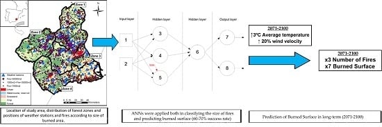
Graphical Abstract

1. Introduction

A wildfire is a fire that spreads without control in forest land [1], where it consumes plant-based biofuels. Fire is an important issue in many forests [2] and has a great influence on forest ecosystems [3], the economic role of forests [4], and human life and health [5,6,7,8]. Its spread depends on climatic conditions, area, topography, vegetation, infrastructure proximity, etc., and its behavior largely varies with forest landscapes [9]. Furthermore, the prediction of the size of a fire is especially important in the allocation of resources for each fire [10]. Fire in Mediterranean regions has become a serious problem in the last three decades, and it is nowadays the main cause of forest loss with an average loss of 5000 km2 per year [11]. Indeed, San-Miguel-Ayanz et al. [12,13,14] have significant knowledge in the analysis, monitoring, and impacts of fire activity in the Mediterranean region. The necessary elements for a fire to occur are known as the “fire triangle” [15,16]. In the simplest form, these elements are fuel, oxygen, and heat. A fire occurs when these features are combined in adequate proportions. Once the fire has started the “fire behavior triangle”, which comprises fuel, topography, and weather, determines how a wildfire behaves. Moreover, concerning forest fires, there are multi-scale triangles where the dominant factors that influence the control of fire behavior depend on the space and time scales considered [17]. Indeed, fire activity is strongly influenced by four factors: weather/climate, fuel, ignition agents, and humans [18,19,20]. Anthropogenic activity is responsible for more than 80% of wildfires in Spain [21]. In fact, the increase in fire numbers from the second half of the 1600s represents an increase in anthropogenic fires [22] with a double contribution: as land use/land change drivers and as cause of fire ignition [23].
The presence of people [24] combined with certain climate conditions determine the ease of wildfire ignition [25]. Climate is a dynamic element, and it has recently been warming due to an increase of greenhouse gases as a result of human activities [26]. This climate change, which is modeled by general circulation models (GCMs), may result in a profound impact on wildfires all over the world [27]. Hence a fire prediction model would make the use and distribution of fire equipment resources more efficient relative to the difficulty of the uncertainty related to human behavior. The ability to predict area burned is crucial to mitigating the immediate and far-reaching consequences of wildfires [28]. Mathematical models have been commonly used in fire prevention, but predictive techniques allow fire prevention authorities to assess the probability of forest fires in the fastest and most effective way [28]. Furthermore, short- or long-term time scales in forest fire risk models can be devised. Long-term models focus on environmental structural characteristics with low variations over time and with higher utility at preventing fires. Most previous research has been focused on changes in fire activity according to climate change [20,29,30,31]. These works indicated that there will be a high increase of fire activity with significant variations at the local scale without changes or even a decrease in fire severity and the number of fires [32,33].
Numerous methods have been applied in order to estimate future fire activity and area burned such as models using dynamic vegetation, landscape fire models [34,35], or relationships between historical area burned and weather [33,36,37]. Dickson et al. [38] focused their research on wildfires greater than 0.2 km2 using Bayesian network analysis and concluded that the occurrence of forest fires was highly correlated with highland mountain zones and low road density. Chou et al. [39] used logistic regression in California using topographic, land-use, and infrastructure location data. Likewise, Cardille et al. [40] and Syphard et al. [41] distinguished between logistic or Poisson regression if the objective was fire probability or number of fires, respectively. Catry et al. [42] also separately used logistic regression in Portugal in fires of more than 5 km2, concluding that these wildfires are more likely to occur in low populated and far-away places. In the last decades, there have also been many studies of wildfires in Spain. For instance, Gallardo et al. [43] used the logistic regression analysis to quantify changes in future fire occurrence due to future land use/land cover variations, Marcos et al. [44] and Turco et al. [29] explored the prediction of summer wildfires by developing a multiple linear regression model, Martin et al. [45] employed the maximum entropy algorithm to analyze the intra-annual dimension of fire occurrence, Ríos Pena et al. [46] explored the use of binary structured additive regression for prediction of wildfires, and Rodrígues et al. [47] assessed the spatial-temporal changes in the contribution of wildfire drivers using geographically weighted logistic regression models. Concerning artificial intelligence techniques, Vasconcelos et al. [48] obtained better results using an artificial neural network (ANN) than logistic regression. Indeed, in recent years computational intelligence models have often been used to perform forest fire prediction [10]. Iliadis [49] created software using fuzzy logic for the prediction of fire risk in Greece. Cheng and Wang [50,51] used data-mining techniques and an ANN to estimate the burned area in Canada. Cortez and Morais [52] estimated forest fire loss in Portugal using multivariate regression, decision trees, random forest, an ANN, and a support vector machine (SVM), obtaining the best results with SVM. Castelli et al. [28] used genetic programming in Portugal, too. Sakr and Elhajj [53] also applied an ANN and an SVM in Lebanon using only humidity and precipitation as inputs. Özbayoğlu and Bozer [10] investigated the size of a fire after its first breakout through an ANN, radial basis function networks, an SVM and fuzzy logic. The ANN model with humidity and wind speed as inputs, and three clusters (small, medium, and big fires) proved to be the best model. Bisquert et al. [54] compared an ANN model and logistic regression to assess forest fire danger. Their results showed good achievements by the ANN technique. Similar results were obtained by Goldarag et al. [55] and Maeda et al. [56], who employed ANNs to identify high forest fire risks in Iran and Brazil, respectively. Satir et al. [57] employed an ANN in a Mediterranean forest ecosystem in Turkey with a coefficient of accuracy of 0.83.
This paper investigated the performance of an ANN in burned area size prediction in a semi-arid region in the south-east of Spain and to assess future evolution of big fires in the area concerned under two climate change scenarios. The contents of the paper are structured as follows: data, study area and methodology are shown in Section 2. Section 3 presents results, which are discussed in Section 4. Finally, Section 5 highlights the main conclusions. This work complements a previous study carried out by Pérez-Sánchez et al. [58] where fire weather indices were assessed in the study area.

2. Materials and Methods

2.1. Data

2.1.1. Study Area

The study area (Murcia) is in southern Spain (Figure 1) and has an area of 11,314 km2. Elevations vary between 0 and 2027 meters above sea level, though 81% of the entire surface is below 1000 m. There is a Mediterranean climate characterized by mild winter, warm and dry summer, and irregular equinoctial rainfall. Annual average precipitation is around 300 mm/year. Temperatures in summer can reach 40–45 °C, resulting, along with spring, in the main seasons for forest fires in the region.
Concerning forest management, four zones have been delimitated by regional and national agencies according to ecologic, socioeconomic, administrative, and physiographic features. Vegetation (Figure 1) is highly influenced by climate. A total of 12% of the surface is used for irrigation cultivation, 40% is used for dry farming, and 48% is occupied by forest, mainly pine forests alternated with scrub, bush, and grassland in proportions greater than 20%, especially in coastal areas. A more accurate description can be seen in the work of Pérez-Sánchez et al. [58].

2.1.2. Wildfire Records

The wildfire database comprises 15 years (2000–2014) and was established by the Forest Authority of Murcia in 2000. The database includes day and hour of the wildfire, location, burned area, causes (real and presumed), type of vegetation, previous wildfires in the area, and relationships with soil conditions. In the 2000–2014 period, 2694 forest fires were recorded in the region with a total burned area of 39.41 km2. Table 1 shows the main characteristics of the wildfires in the region in the studied period (2000–2014). More than 75% of the burned surface is located only in forest areas, as can be seen in Figure 1. Although the surface of all zones is between 2500 and 3500 km2, the number of wildfires and burned area varies widely depending on the zone itself and its geographical, climatic, and ecological characteristics more than its extension. Zone 4 has the lowest number of fires of the region (20.49%) but, on the contrary, its burned area in the studied period is the highest (45.18%), since the mean ratio of m2 per fire is 32,261 m2/fire versus the 6327 m2/fire of Zone 1, which has the highest amount of fires (43.28%). Furthermore, despite Zones 2 and 3 having similar surfaces (2378.50 and 2439.53 km2, respectively) and similar numbers of wildfires (614 and 661, respectively), the burned area in Zone 2 is nearly triple that of Zone 3 (26.64% and 9.46%, respectively). All zones show similar values for 50th, 75th and 95th percentiles (around 1000, 5000, and 20,000 m2, respectively) except Zone 4 where the burned area in the studied period is significantly higher than the rest of the region.
Concerning the size of the fires, although more than 94% of fires in all zones were below 30,000 m2 of burned area (histogram in Figure 1), the remaining 6% of fires accounted for almost 80% of the total burned area in the region in the studied period. This fact clearly points to the importance of big fires in the forest ecosystems and their subsistence and whose impacts transcend the damage and degradation of ecosystems and material properties, especially in semiarid regions [58].

2.1.3. Weather Stations

The present study is mainly based on meteorological factors and indices related to them. The data used in this study come from 39 weather stations (Figure 1) operated by the Murcian Institute of Agricultural Research and Development and Food. Each station comprises a database with records of daily rainfall (mm), temperatures (°C), relative humidity (%), and wind speed (m/s) during the 2000–2014 period. Annual precipitation in the region is on average 270 mm, average relative humidity ranges between 60% and 70%, and the average temperature varies between 13 °C in the northwest and the 18 °C in the southeast. These values are higher than in the rest of the region in Zone 4, especially in spring and summer favoring wildfires, which is also due to the scarcity of rainfall events. Wind speed depends on altitude, and the highest values are reached on mountain range peaks.
A combination of the Global Climate Model (GCM) EC-EARTH and the Regional Climate Model (RCM) HIRHAM5 was downloaded from the EURO-CORDEX initiative [59] to simulate future scenarios and to assess climate change consequences in the region for the period 2071–2100 under two different representative concentration pathway (RCP) emission scenarios (RCP4.5 and RCP8.5). These scenarios assume pathways to different target radiative forcing at the end of the 21st century [59]. For example, scenario RCP4.5 figures that an increase in radiative forcing of 4.5 W/m2 can be produced by the end of the century relative to preindustrial conditions. Senent-Aparicio et al. [60] applied the Fuzzy TOPSIS technique to rank a set of nine GCM-RCM combinations in the study area, obtaining that the combination of EC-EARTH and HIRHAM5 provides a good fit to the observed meteorological variables during the control period. A bias correction technique based on distribution mapping of variables was applied to the downscaled data to increase the accuracy of the results. This process adjusts the cumulative distribution function of the forecasts to the observed one by applying mapping functions between the corresponding quantiles. We used the R free software and the contributed package “qmap” [61], which can be obtained from the R project website.

2.1.4. Fire Weather Indices

Previous studies [46] have demonstrated that the Forest Weather Index (FWI) [62,63] appears to be the most suitable index in a semiarid region. Furthermore, the Angström Index (AI) [64] can identify fire-danger warnings in the driest and highest temperature areas. Thus, both indices have been taken into account in the present research.
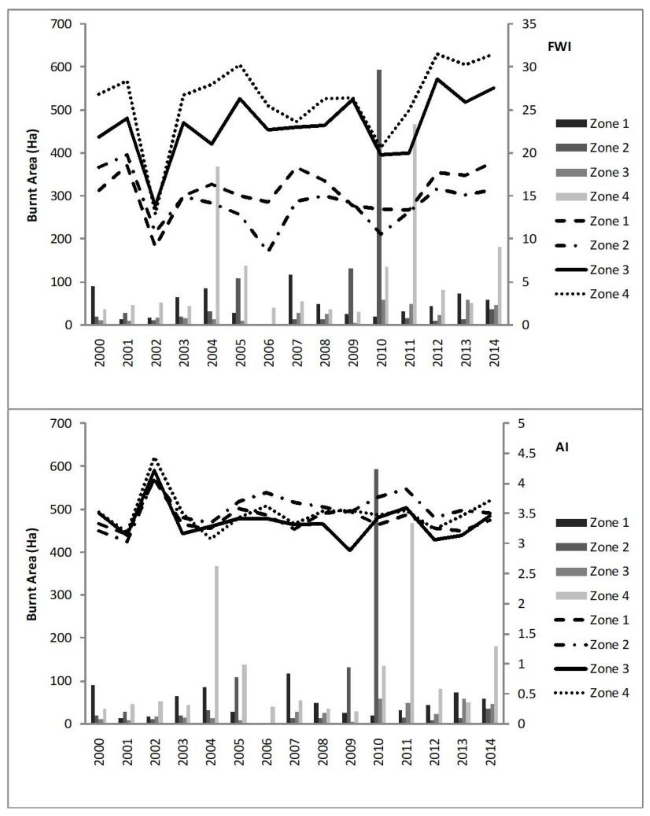
AI only considers temperature and relative humidity, whereas FWI [65] takes into account weather conditions and their relationships with soil moisture and fire activity. Regarding the period, AI considers a one day-period whereas FWI is accumulative and considers longer periods depending on the previous index values. Concerning the fire occurrence, the lower the value of AI, the higher the probability of fire occurrence, especially for AI < 2; on the contrary, the higher the value of FWI, the more likely a wildfire is to occur, especially when FWI > 16. As it can be seen in Figure 2, despite FWI being the most suitable index to predict a fire day in the study area, the index itself does not show a clear pattern related to burned area, though its minimum values usually match with the years of smallest burned area. However, the further southeast the area is (Zones 3 and 4), the higher the FWI is, on average, on a fire day (around 25). AI seems to be more stable and its range remains around 3.5 in the studied period, with relative maximums on non-fire days, but it is not able to detect the burned area extension by itself. Nevertheless, both indices were taken into account combined with weather, temporal, and geographical variables in the present study due to their suitability in fire day prediction.
Package “fireDanger” [66,67,68] from the R statistical software [69] was used in the calculation of FWI and AI for both 2000–2014 and 2071–2100 periods.

2.2. Methods

As stated above, this paper investigated the performance of an ANN in burned area size prediction to assess future evolution of fires under climate change conditions. Figure 3 summarizes the proposed methodology. The first step was to establish a fire size threshold to assess the broken up burned surfaces and classify them according their burned area. Daily rainfall (P), average temperature (T), relative humidity (H), and wind speed (V) were evaluated daily for all the wildfires during the 2000–2014 period using the Kriging method. Likewise, FWI and AI were assessed for all the fire record datasets. The fire size threshold to differentiate homogeneous classes was established as 30,000 m2 using a cluster analysis with the previous variables and the coordinates of the wildfire (X, Y Z), the month of the year (M), and the type of vegetation. The goals of the second step were, for the two RCPs in the 2071–2100 period: (1) to determine the day and location of a wildfire in the future depending on the FWI and AI indices obtained, (2) to classify the detected wildfires according to the threshold of 30,000 m2 and (3) to predict the size or burned surface for wildfires larger than 30,000 m2. The latter two stages were performed with ANN.

2.2.1. Database

Initially, and with the goal of considering the maximum of the meteorological variables in the study, P, T, H, and V were evaluated daily for all the wildfires during the 2000–2014 period. Although spring and summer were the seasons with the highest number of big wildfires in the 2000–2014 period, data for the entire year were used in this study to analyze future variations in the risk period of forest fires. The Kriging technique [70,71] was applied to obtain these values for fire days in forest fire locations. The Kriging method performs better than non-geostatistical methods [72] and has strong theoretical support [70]. Ordinary Kriging and a hypothetical spherical variogram [73] were used with ArcMap 10.2 [74] in this study.
Thus, the database used for this study for each of the four zones is comprised by the variables shown in Table 2.

2.2.2. Cluster Analysis

After selecting the input variables, a non-hierarchical cluster analysis was performed in order to obtain the centroids of the most homogeneous groups of fire events in each zone and to assess the broken up burned surfaces to classify them according their burned area. The k-means algorithm [75] was used due the possibility of assigning objects to a user-defined number of clusters (k) in such a way as to minimize the sum of intra-cluster distances between the object and the centroid of its cluster. The k value was assessed for clusters of three, four, and five objects, and the results are shown in Table 3.
Centroids obtained establish different thresholds depending on the burned surface (among other factors) and number of fires related to each zone. Thus, due to higher mean and maximum burned areas in Zones 2 and 4 (Table 1) than Zones 1 and 3, the former zones have higher values for all the clusters, especially the highest ones. Nevertheless, the lowest categories are all fairly similar. The first two centroids’ values are around 2000–8000 m2 and 25,000–40,000 m2, respectively, which is not found in the rest of them. In view of the results, fires were divided into two main categories, big fires and small fires, and 30,000 m2 of burned area in a single fire was considered as the threshold of classification. This classification is in line with the recommendations of the now-defunct Institute for the Preservation of Nature of Spain [76], which established 50,000 m2 as the threshold to differentiate large or small fires. Actually, despite the large number of wildfires in Spain in the last decades, only a small number of cases, the “huge fires” [77], are responsible for the majority of losses. Likewise, recent Spanish studies [29,78] propose similar classes to obtain homogenous series [29]. Moreover, in the studied region, as can be seen in Table 1, fires larger than 30,000 m2 covered nearly 80% of the total burned area in the region during the studied period, and their prediction and evolution was therefore the goal of this study.

2.2.3. Artificial Neural Network (ANN)

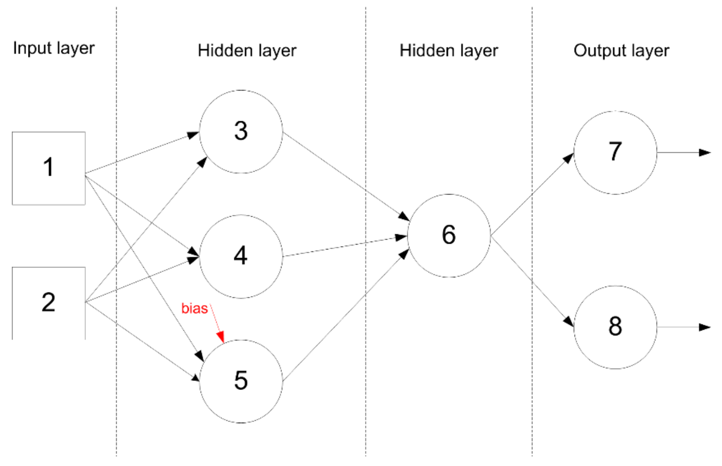
An ANN is a computational method based on the behavior of the human brain, mainly the nervous system and its connections. It therefore creates artificial models or patterns which deal with problems difficult to solve using conventional algorithm techniques. ANNs are considered nonlinear statistical data tools that can learn, memorize, and disclose the different relations in data. They model complex relationships between input and output data of an area regardless of the physical features involved. They consist of a group of units called neurons that are connected each other through several links to transmit signals. The multilayer perceptron [79] is one of the simplest and most commonly used architectures in ANNs in data analysis [80], and it was used in the current study. This model consists of several computational layers interconnected to each other where each artificial neuron (or perceptron) is directly connected to each one of the adjacent layer (Figure 4). The input data are introduced into the network through the neurons of the input layer. The hidden layers comprise neurons whose inputs come from previous layers and whose outputs go to subsequent layers. Finally, the output layer provides the outputs for the given inputs. All neurons have a bias weight. Except for the input nodes, where the information is only processed, each neural network uses as an activation function a sigmoidal function in hidden layers and a softmax function or lineal function in the output layers.
The mathematical expression of a neuron is given as Equation (1):
y i = f ( i = 1 N x i · ω i b j ) ,
where y is the output of a neuron j, f is an activation function, xi is an input of the vector of inputs (i = 1, 2,..., N), ωi is the weight associated with the connection link through which the input xi arrives to current neuron j from a neuron in the preceding layer, and bj is a bias associated with neuron j. The training process consists of varying weights and biases on the basis of the given inputs and aims based on the performance measure.
This study used an ANN for two purposes and subsequential phases. The first phase was to classify the size of the wildfires, distinguishing between big fires (more than 30,000 m2) and small fires, which do not exceed 30,000 m2 of burned area in a single wildfire. In the second phase, once wildfires were classified according to the burned area, an ANN was used to predict the burned surface for only big fires, since they account for more than 80% of the burned area in the region. Both phases consisted of three stages required for ANNs: training, validation, and testing. The aim of network training is for the ANN to be capable of reproducing the behavior of input data predicting relationships not found before by minimizing an error function. Different types of learning algorithms are used for the training stage. In this study, a backpropagation algorithm was used to train. The output errors between the output and actual target (observed data) are repeatedly propagated backwards through the network to modify weights and bias parameters. The training stage is finished when the error on the validation dataset is near minimum. The superiority of the Levenberg–Marquardt (LM) algorithm [81,82] has clearly been shown in different studies [83,84]. Therefore, LM is usually the fastest backpropagation algorithm. Different types and numbers of inputs (within the variables in Table 2) were employed in the ANN to estimate outputs in each phase.
Most learning systems are not prepared to cope with unbalanced data such as shown in Table 1 for the uneven distribution of burned areas, and various methods have been proposed. Over- and under-sampling methodologies have been extensively discussed to assess the effect of imbalanced datasets [85,86,87,88]. Various studies have brought to light the usefulness of oversampling versus under-sampling [87,89,90]. In this study, the function ubOver from the package ‘unbalanced’ [91] from the R statistical software [69] was used. It replicates randomly some instances from the minority class in order to obtain a final dataset with the same number of instances from the two classes.

2.2.4. ANN Classification Performance Evaluation Methods

Four methods were used for performance evaluation in ANN classification of big and small fires (larger or smaller than 30,000 m2 burned area, respectively): classification accuracy, analysis of sensitivity and specificity, confusion matrix, and k-fold cross-validation.
  • Classification accuracy
The classification accuracies for the datasets are evaluated using Equation (2):
accuracy T = i = 1 T   asssess ( t i ) T ,   t i T , assess t = 1 ,   i f   c l a s s i f y t c o r r e c t c l a s s i f i c a t i o n 0 ,   o t h e r w i s e ,
where T is the test set, t ∈ T, ti is the class of item t, and classify(t) returns the classification of t by ANN classifier.
  • Sensitivity and specificity
Sensitivity and specificity analysis are shown in Equations (3) and (4), respectively:
sensitivity = T P T P + F N   %
specificity = T N F P + T N   %
where TP, TN, FP, and FN are true positives, true negatives, false positives, and false negatives, respectively.
  • Confusion matrix
The confusion matrix [92] matches the predicted and actual values and was selected as a measure of goodness-of-fit for the first phase of distinguishing wildfires larger and smaller than 30,000 m2. A confusion matrix of class n is a matrix of size n × n where the rows are named according to real classes and the columns according to predicted classes. Table 4 shows a confusion matrix for n = 2, where a, b, c, and d are the numbers of real negative predictions, false positive predictions, false negative predictions, and correct positive predictions, respectively.
  • k-fold cross-validation
k-fold cross-validation divides the dataset randomly into k subsets of the same size. Each time, k − 1 subsets are used in the training set and the remaining k subset is used as the test set. The process is repeated k times with each of the k subsets, using a different subset as test set in each iteration. This process generates k estimations of the error test whose average is computed as the single estimation, using all observations for both training and calibration phases and each observation is used for validation only once. A 10-fold cross-validation is often used [93].

2.2.5. ANN Burned Area Prediction Metrics

The models obtained for prediction of burned areas in big wildfires (larger than 30,000 m2) for each zone were analyzed using four error metrics based on the deviation from target for the actual burned area: mean absolute deviation (MAE) (Equation (5)), root mean square error (RMSE) (Equation (6)), mean absolute percent error (MAPE) (Equation (7)), and the bias (Equation (8)) defined by Pielke [94] and Stauffer and Seaman [95] in order to measure the accuracy of the simulation:
M A E = i = 1 N y i t i N
RMSE = i = 1 N y i t i 2 N
M A P E = i = 1 N y i t i y i N x 100
B i a s = i = 1 N   y i t i N
where yi is the predicted value, ti is the target value, and N is the number of analyzed values.
MAE, RMSE, and bias are expressed in the same units as the studied variable (m2 of burned area) whereas MAPE shows the goodness-of-fit as a percentage of the error. Outliers have more effect in RMSE than MAE, therefore it will give more weight to higher difference values. Bias provides information related to the tendency to overestimate or underestimate the target value, quantifying the model systematic error.

3. Results

3.1. Climate Change

In order to establish relationships between predicted burned area and climate change meteorological data, Table 5 shows the average values of P, H, T, and V for the 2000–2014 period and 2071–2100 period in both selected scenarios (RCP4.5 and RCP8.5). These scenarios assume pathways to different target radiative forcing at the end of the 21st century [59]. For example, scenario RCP4.5 figures that an increase in radiative forcing of 4.5 W/m2 can be produced by the end of the century relative to preindustrial conditions. Both precipitation and humidity remain invariable in the four zones due to their proximity. Future average values for precipitation are always higher than in the last 15 years of historical available data (2000–2014), reaching an average increase around 20% of rainfall, except in the wettest zone of the region (Zone 2) where there is a slight decrease of 3% in the RCP8.5 scenario. Average temperature rises between 2 and 4 °C in RCP4.5 and RCP8.5, respectively, in all zones, except in Zone 2 where the temperature increase is even higher, more than 6 °C in the RCP8.5 scenario. As a result of this overall increase in the region, climatic differences between zones are reduced at the expense of global warming. Another important factor of burned area fire size is wind velocity, which is also increased in all regions an average of 15–25%, especially in northwest-southeast direction due to the mountain ridges in this direction [58].
Considering that fire conditions are very favorable when FWI > 16 [63,65], in Table 6 a comparison is shown between the number of fires in the available data series period (2000–2014) and predicted fires for both future scenarios (RCP4.5 and RCP8.5) in the long-term period (2071–2100).
The results indicate that the number of fires in the future for both scenarios will significantly increase in all zones except Zone 3 and the RCP4.5 scenario, where the number of fires appears to be similar to the number recorded in the 2000–2014 period. However, the RCP8.5 scenario doubles the number of fires per year in all zones, even tripling the number in Zone 4, moving up from an average of 37 fires per year in the period 2000–2014 to 106 fires per year, on average, in the long term (2071–2100).

3.2. Classification of Fires

The effectiveness of ANNs to classify fires in each zone during the studied period was applied to the database described in Section 2 and with the variables shown in Table 2. The subset of fires larger than 30,000 m2 (big fires) was extended with the oversampling technique to balance with the fires smaller than 30,000 m2 (small fires) data subset. The experiments demonstrated the lesser importance of coordinates, altitude, and vegetation in each of the four zones, so these variables were removed in subsequent analysis. AI only showed its relevance in Zone 4, so it was used just for this area. Thus, the variables considered in the study were finally: month, H, T, V, FWI and, in Zone 4, also AI. It is important to note that Precipitation is part of both FWI and AI indices. In order to improve the robustness and stability of results and to reduce bias, five partitions in the dataset were made (50–50%, 60–40%, 70–30%, 80–20%, and 90–10% in training-test, respectively).
The obtained classification accuracy and values of sensitivity and specificity by the ANN classifier for size of wildfire with mentioned partitions are shown in Table 7. Sensitivity defines the proportion of true positive big fires detected in the total group of real big fires. Actually, it can be considered as the probability of getting a positive test result in big fire datasets. Hence, it relates to the potential of the test to recognize big fires. All regions showed an average sensitivity percentage higher than 60%, even reaching 70% in Zone 3, but in Zone 4 the average reached around 55%. This was likely due to the fact that Zone 4 is the most populated zone (coastal area) of the region and lower values of sensitivity might indicate a greater relevance of anthropogenic causes. The same pattern with higher values, especially in Zone 4, is shown for the specificity measure. It defined the proportion of small fires detected that are really burned fire areas below the threshold of 30,000 m2.
Specificity is complementary to sensitivity and provides the probability of a non-big fire in a small fire dataset. In other words, it relates to the aspect of the test’s ability to recognize small fires (i.e., to exclude the condition of interest). Specificity in the four zones is around 70%. Finally, the average accuracy of tests in the four zones varies in the range of 60–70%. As Table 6 shows, the higher the training rate is, the better are results achieved for all these measures of evaluation, until the test partition percentage decreases below 20%, where accuracy even exceeds 80% in Zones 2 and 3.
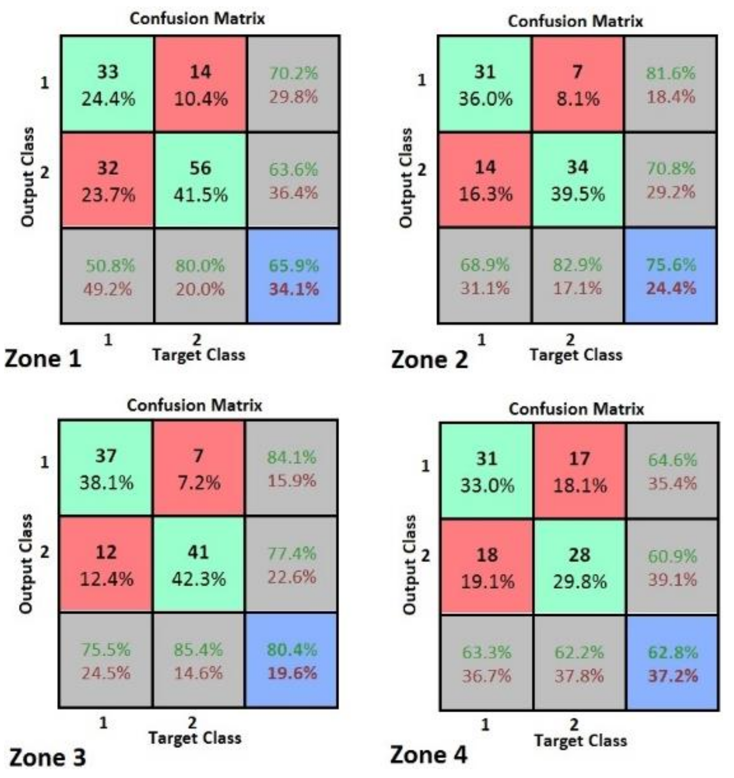
Three matrices of confusion (training-validation-test) were obtained for each zone depending on the partition considered. As a result, 60 matrices of confusion were used in the study. For example, in Figure 5, the test matrix of confusion for each zone of the region is shown for the 80–20% training-test partition, where along the x-axis the true class labels are listed and along the y-axis are the nearest neighbors’ class predictions. Along the first diagonal are the proper classifications, whereas all the other entries show incorrect classifications. The bottom right value indicates the overall accuracy. Class 1 represents fires smaller than 30,000 m2 of burned surface, and class 2 is the ones larger or equal to 30,000 m2. Regarding matrices of confusion, they not only show the measures of accuracy of tests results (Table 7) but also the number of fires within each subset in every partition taken into account, as well as successes and errors in absolute terms, considering the oversampling carried out on the big fire dataset.
Finally, to improve over the hold-out method, 10-fold cross-validation was conducted in the classification study and the results are shown in Table 8. The average values obtained are in line with the previous goodness-of-fit tests carried out. Zones 1 and 4 results show, on average, 61% and Zones 2 and 3, 74% and 69%, respectively. Notwithstanding this difference, the standard deviation is nearly one-half (around 5%) higher in the former than in the latter, which leads to the consideration of an overall performance of the method around 65% in the region.

3.3. Burned Area Prediction under Climate Change

After having classified wildfires into two main classes (big and small wildfires), an ANN was used to predict fires of burned area equal or larger than 30,000 m2. In this case, the dataset was divided into three sections. Sixty percent of the data was used for training purposes, 20% was used for validation, and the remaining 20% was reserved for testing [10]. The variables considered in prediction were M, H, T, V, FWI, and AI. Table 9 shows the results of all metrics considered in each region for all the partitions described. MAE and RMSE values are higher, and relatively similar, in Zones 1 and 4 but total burned areas in these zones are significantly different, practically double that in Zone 4. In fact, the sum of RMSE in the three partitions represents 5.64% and 1.85% of the total wildfire surface for big fires in Zones 1 and 4, respectively. Likewise, Zones 2 and 4 have a similar behavior for the same metrics and similar percentage of sum of RMSE to burned surface, resulting in 3.77% and 3.62% in Zones 2 and 4, respectively, since the burned area in big wildfires in these zones differs by less than 20%.
MAPE percentages range from 11% to 43% in the training set and from 19% to 40% in the test set. Zone 3 remains invariable in partitions within the range of 12–20%, whereas the rest of the zones show wider variations, especially Zone 2. Nonetheless, test values do not exceed 40% or even reach around 20% in Zones 1 and 3. Concerning bias, the ANN model tends to underestimate burned surface by around 20% on average for the whole region, though it varies, both overestimating and underestimating, depending on the partition and zone under study.
Burned surface over the long-term period (2071–2100) increases hugely in all zones (Table 10). Average yearly values are up to 12 times (or even more depending on the climate scenario) higher than recorded wildfires in the period under study (2000–2014) in Zone 3. Increases of burned surface in the rest of the zones are lower, but they are up to five times higher as is the case of Zone 1. It appears to be a reduction in the variance between zones and a tendency to a homogenization at the regional level except for Zone 4, where, despite being the area most affected by wildfires, burned surface does not increase five-fold in the pessimistic scenario.
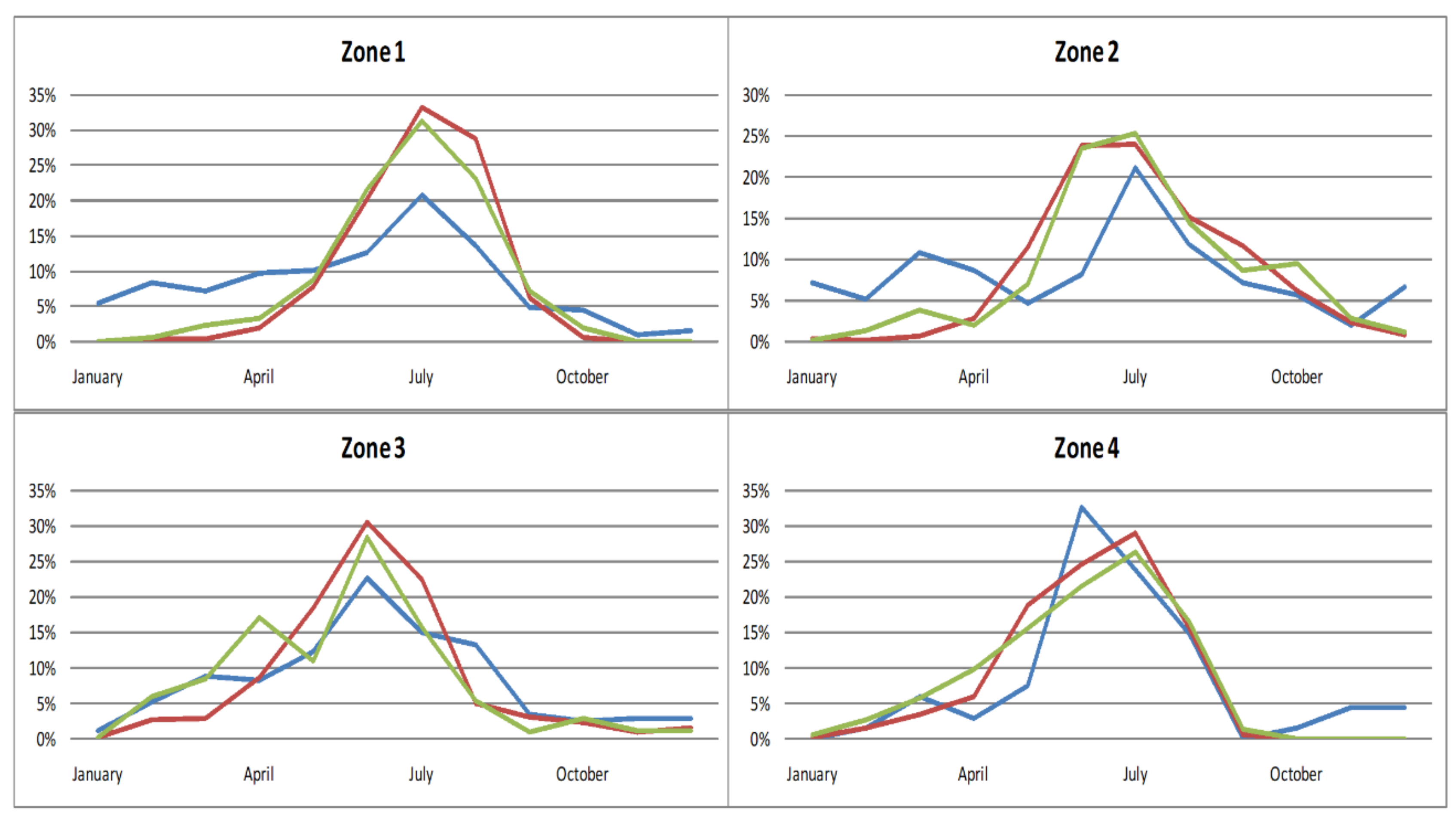
Concerning seasonal variations (Figure 6), while at the moment risk period generally lasts from March to September with peaks in June (Zones 3–4) or July (Zones 1–2), predicted wildfires in long-term period are mostly confined in the summer season, especially in June and July months, which means that the high-risk period is shortened but total burned surface significantly increases, especially in Zone 1. In fact, big wildfires in autumn and winter are limited to their proximity with spring or summer and are rarely to happen. Zone 4 moves its maximum from June to July, consistent with the rest of the region. The patterns for RCP4.5 and RCP8.5 are rather similar with more pronounced changes in RCP4.5 during the year.

4. Discussion

The behavior of wildfires in the studied region is very sensitive to burned surface area. The patterns of fires are strongly linked to meteorological variables depending on burned surface area. The k-means algorithm is capable of establishing the thresholds of all factors taken into account and differentiates the clusters in which fires in each zone can be divided. Wildfires with burned surfaces larger than around 30,000 m2 account for more than 80% of the total burned area in the dataset period (2000–2014) and appear to be in all zones as the threshold that makes the difference between small and big fires. Small fire clusters do not follow a clearly identifiable pattern with used techniques, but the ANN method proved satisfactory results in wildfires with burned surfaces greater than 30,000 m2.
Analysis of climatic, ecological, and geographical variables carried out by an ANN reject geographical and ecological factors’ influence in big fires, possibly due to little change in ecosystems in the four zones, albeit local variations of forests of pine alternated with areas covered in scrub, bush, and grassland in proportions greater than 20%, especially in coastal areas. Furthermore, an extension of 11,314 km2 with geographic coordinates in a range of 1° of latitude (between 38°45′N and 37°23′N) and less than 2° of longitude (between 0°41′W and 2°21′W) and a topography whose valleys and plains account for 75% of the total region has a reduced impact on burned surface. Therefore, the variables finally used in this study were precipitation, relative humidity, wind speed, temperature, and the weather fire indices FWI and AI, though the latter, in the ANN classification, only influences Zone 4 as it had already been reflected in the previous study of Pérez-Sánchez et al. [58], owing to higher yearly maximum temperatures in southern areas.
Increase in precipitation around 20% in both climate change scenarios will not by itself reduce the total burned surface because a rising temperature of 3 °C, on average, cannot be compensated with regard to ignition and fire spreading. Furthermore, wind velocity proves to be a relevant factor as it was suggested by Özbayoğlu and Bozer [10]. An increase of 15–25% in wind speed, apart from increasing temperature, leads to double the number of fires per year in all zones and even to triple in Zone 4, where the increase of temperature is maximum, around 4 °C in the RCP8.5 scenario.
The performance of ANNs in classifying the size of fires was assessed using different partitions in training-test datasets (from 50–50% to 90–10% in training-test, respectively). Furthermore, various evaluation criteria were also used, providing more robustness and accuracy to results obtained. The higher the training rate is, the better are the results achieved for all measures of evaluation, until the test partition percentage decreases below 20%, though accuracy even exceeds 80% in Zones 2 and 3 at the expense of greater variance. ANN classification showed good sensitivity, specificity, and accuracy in all zones reaching percentages between 60% and 70%. Likewise, 10-fold cross-validation results were in line with previous goodness-of-fit tests, leading to an overall performance of the classifying method around 65% in the region. Burned surface prediction by ANNs show a significantly increase of burned area under both climate change scenarios. In fact, the straightforward view of a warming climate affecting fire regimes is supported by scientific literature [96], finding wide agreement of projections of increased area burned [97] of up to two- to five-fold increases in annual area burned under a moderate warming scenario [98]. In the region under study, yearly average predicted burned surface depends both on the climate scenario and on the zone, and it ranges from four times (Zone 4) to 12 times (Zone 3) higher than datasets recorded for the period 2000–2014. Statistics indicate that the error in burned surface prediction is below 40%, and it is generally underestimated around 20%, which may lead to worse consequences than expected. Nevertheless, the highest risk season is shortened to late spring and summer, and an overall reduction in fire cycles is predicted, as suggested by Westerling et al. [99].

5. Conclusions

The prediction of the size of a fire is especially important in the allocation of resources in each fire. Wildfires larger than 30,000 m2 in the study area in southern Spain represent only 6% of the entire record for 2000–2014, but they account almost 90% of the total burned area, thus the prediction and evolution of these ‘big’ fires are a key issue in firefighting. ANNs were applied both in classifying the size of fires and predicting burned surface with good performance in all zones in the studied region. The results indicate that the estimation process was always above 60%, reaching more than a 70% success rate in the central area. General warming of 3 °C and an increase of 20% in wind speed in the long-term period (2071–2100) will result in three times the number of fires and a significant increase of yearly average burned surface up to 12 times depending on the zone and the climate change scenario, though the high-risk season is shortened. These estimates do not take into account anthropogenic changes (land use activities, fire management, or public awareness) which could influence areas burned. The methodology used can be applied in semi-arid regions with similar case studies in order to assess the adequacy of staff and equipment in the control of forest fires.

Author Contributions

All authors equally contributed to conceiving and designing the experiment; J.P.-S. and P.J.-S. performed the experiments; J.S.-A., J.M.D.-P. and J.d.D.C.-C. analyzed the data; all authors contributed to writing and revising the manuscript.

Funding

This research was funded by the Region of Murcia Government. (Grant # GR-2016/043998).

Acknowledgments

The authors gratefully acknowledge support from the Region of Murcia Government through the project “Validación de diferentes indices de predicción de incendios en la Región de Murcia”. We also acknowledge Papercheck Proofreading and Editing Services.

Conflicts of Interest

The authors declare no conflict of interest.

References

  1. Molina, D.; Blanco, J.; Galan, M.; Pous, E.; García Jurado, J.; García Jurado, D. Incendios Forestales: Fundamentos, Lecciones Aprendidas y Retos de Futuro; Ed. AIFEMA: Granada, Spain, 2009. [Google Scholar]
  2. Moritz, M. Spatiotemporal analysis of controls on shrubland and fire regimes: Age dependency and fire hazard. Ecology 2003, 84, 351–361. [Google Scholar] [CrossRef]
  3. Minnich, R.A.; Bahre, C.J. Wildland fire and chaparral succession along the california-baja california boundary. Int. J. Wildland Fire 1995, 5, 13–24. [Google Scholar] [CrossRef]
  4. Hardy, C. Wildland fire hazard and risk: Problems, definitions and context. For. Ecol. Manag. 2005, 211, 73–82. [Google Scholar] [CrossRef]
  5. Analitis, A.; Georgiadis, I.; Katsouyanni, K. Forest fires are associated with elevated mortality in a dense urban setting. Occup. Environ. Med. 2012, 9, 158–162. [Google Scholar] [CrossRef] [PubMed]
  6. Jayachandran, S. Air quality and early-life mortality: Evidence from Indonesia’s wildfires. J. Hum. Resour. 2009, 44, 916–954. [Google Scholar] [CrossRef]
  7. Vedal, S.; Dutton, S.J. Wildfire air pollution and daily mortality in a large urban area. Environ. Res. 2006, 102, 29–35. [Google Scholar] [CrossRef] [PubMed]
  8. Bowman, D.M.J.S.; Johnston, F.H. Wildfire smoke, fire management, and human health. EcoHealth 2005, 2, 76–80. [Google Scholar] [CrossRef]
  9. Reed, W.J.; McKelvey, K.S. Power-law behaviour and parametric models for the size-distribution of forest fires. Ecol. Model. 2002, 150, 239–354. [Google Scholar] [CrossRef]
  10. Özbayoğlu, A.M.; Bozer, R. Estimation of the Burned Area in Forest Fires Using Computational Intelligence Techniques. Procedia Comput. Sci. 2012, 12, 282–287. [Google Scholar] [CrossRef] [Green Version]
  11. Vélez, R. Causes of fires in the Mediterranean basin. EFI Proc. 2002, 45, 35–42. [Google Scholar]
  12. San-Miguel-Ayanz, J.; Pereira, J.; Boca, R.; Strobl, P.; Kucera, J.; Pekkarinen, A. Forest fires in the European Mediterranean region: Mapping and analysis of burned areas. In Earth Observation of Wildland Fires in Mediterranean Ecosystems; Chuvieco, E., Ed.; Springer: Berlin/Heidelberg, Germany, 2009; pp. 189–204. [Google Scholar]
  13. San-Miguel-Ayanz, J.; Schulte, E.; Schmuck, G.; Camia, A.; Strobl, P.; Liberta, G.; Giovando, C.; Boca, R.; Sedano, F.; Kempeneers, P.; et al. Comprehensive monitoring of wildfires in Europe: The European Forest Fire Information System (EFFIS). In Approaches to Managing Disaster–Assessing Hazards, Emergencies and Disaster Impacts; Tiefenbacher, J., Ed.; In-Tech Publishers: Texas State University, San Marcos, TX, USA, 2012. [Google Scholar]
  14. San-Miguel-Ayanz, J.; Moreno, J.; Camia, A. Analysis of large fires in European Mediterranean landscapes: Lessons learned and perspectives. For. Ecol. Manag. 2013, 294, 11–22. [Google Scholar] [CrossRef]
  15. Countryman, C.M. The Fire Environment Concept; U.S. Department of Agriculture Forest Service Pacific Southwest Forest and Range Experiment Station: Berkeley, CA, USA, 1972; Volume 21.
  16. Pyne, S.J.; Andrews, P.A.; Laven, R.D. Introduction to Wildland Fire; Wiley: New York, NY, USA, 1996; p. 769. [Google Scholar]
  17. Moritz, M.A.; Morais, M.E.; Summerell, L.A.; Carlson, J.M.; Doyle, J. Wildfires, complexity, and highly optimized tolerance. Proc. Natl. Acad. Sci. USA 2005, 102, 17912–17917. [Google Scholar] [CrossRef] [PubMed] [Green Version]
  18. Johnson, E.A. Fire and Vegetation Dynamics: Studies from the North American Boreal Forest; Cambridge University Press: Cambridge, UK, 1992. [Google Scholar]
  19. Swetnam, T.W. Fire history and climate change in giant sequoia groves. Science 1993, 262, 885–889. [Google Scholar] [CrossRef] [PubMed]
  20. Flannigan, M.D.; Wotton, B.M. Climate, weather and area burned. In Forest Fires: Behavior & Ecological Effects; Johnson, E.A., Miyanishi, K., Eds.; Academic Press: University of Calgary, Calgary, AL, Canada, 2000; pp. 335–357. [Google Scholar]
  21. DGCN. Los Incendios Forestales en España. Decenio 1996–2005; Dirección General de Conservación de la Naturaleza. Ministerio de Medio Ambiente: Madrid, Spain, 2006. [Google Scholar]
  22. Niklasson, M.; Granstrom, A. Numbers and Sizes of Fires: Long-Term Spatially Explicit Fire History in a Swedish Boreal Landscape. Ecology 2000, 81, 1484–1499. [Google Scholar] [CrossRef]
  23. Bajocco, S.; Ferrara, C.; Guglietta, D.; Ricotta, C. Fifteen years of changes in fire ignition frequency in Sardinia (Italy): A rich-get-richer process. Ecol. Indic. 2019, 104, 543–548. [Google Scholar] [CrossRef]
  24. Wotton, B.M.; Martell, D.L.; Logan, K.A. Climate change and people-caused forest fire occurrence in Ontario. Clim. Chang. 2003, 60, 275–295. [Google Scholar] [CrossRef]
  25. Chuvieco, E.; Aguado, I.; Yebra, M.; Nieto, H.; Salas, J.; Martín, M.P.; Vilar, L.; Martínez, J.; Martín, S.; Ibarra, P.; et al. Development of a framework for fire risk assessment using remote sensing and geographic information system technologies. Ecol. Model. 2010, 221, 46–58. [Google Scholar] [CrossRef]
  26. Intergovernmental Panel on Climate Change. Climate Change 2001 The Scientific Basis; Cambridge University Press: Cambridge, UK, 2001. [Google Scholar]
  27. Flannigan, M.; Stocks, B.; Turetsky, M.; Wotton, M. Impacts of climate change on fire activity and fire management in the circumboreal forest. Glob. Chang. Biol. 2008, 14, 1–12. [Google Scholar] [CrossRef]
  28. Castelli, M.; Vanneschi, L.; Popovič, A. Prredicting burned areas of forest fires: An artificial intelligence approach. Ecology 2015, 11, 1. [Google Scholar] [CrossRef]
  29. Turco, M.; Llasat, M.C.; von Hardenberg, J.; Provenzale, A. Climate change impacts on wildfires in a Mediterranean environment. Clim. Chang. 2014, 125, 369. [Google Scholar] [CrossRef]
  30. Moritz, A.; Parisien, M.A.; Batllori, E.; Krawchuk, M.A.; Van Dorn, J.; Ganz, D.J.; Hayhoe, K. Climate change and disruptions to global fire activity. Ecosphere 2012, 3, 1–22. [Google Scholar] [CrossRef]
  31. Flannigan, M.D.; Stocks, B.J.; Wotton, B.M. Forest fires and climate change. Sci. Total Environ. 2000, 262, 221–230. [Google Scholar] [CrossRef]
  32. Parks, S.A.; Miller, C.; Abatzoglou, J.T.; Holsinger, L.M.; Parisien, M.A.; Dobrowski, S.Z. How will climate change affect wildland fire severity in the western US? Environ. Res. Lett. 2016, 11, 3. [Google Scholar] [CrossRef]
  33. Flannigan, M.D.; Logan, K.A.; Amiro, B.D.; Skinner, W.R.; Stocks, B.J. Future Area Burned in Canada. Clim. Chang. 2005, 72, 1. [Google Scholar] [CrossRef]
  34. Brillinger, D.R.; Preisler, H.K.; Benoit, J.W. Risk assessment: A forest fire example. In Statistics and Science: A Festschrift for Terry Speed; Goldstein, D., Speed, T., Eds.; IMS Lecture Notes Monograph Series; Institute of Mathematical Statistics: Beachwood, OH, USA, 2003; Volume 40, pp. 177–196. [Google Scholar]
  35. Jaiswal, R.; Saumitra, M.; Kumaran, D.; Rajesh, S. Forest fire risk zone mapping from satellite imagery and GIS. Int. J. Appl. Earth Obs. Geoinf. 2002, 4, 1–10. [Google Scholar] [CrossRef]
  36. Birch, D.S.; Morgan, P.; Kolden, C.A.; Abatzoglou, J.T.; Dillon, G.K.; Hudak, A.T.; Smith, A.M.S. Vegetation, topography and daily weather influenced burn severity in central Idaho and western Montana forests. Ecosphere 2015, 6, 17. [Google Scholar] [CrossRef]
  37. Finney, M.A. The challenge of quantitative risk analysis for wildland fire. For. Ecol. Manag. 2005, 211, 97–108. [Google Scholar] [CrossRef]
  38. Dickson, B.G.; Prather, J.W.; Xu, Y.; Hampton, H.M.; Aumack, E.N.; Sisk, T.D. Mapping the probability of large fire occurrence in northern Arizona, USA. Landsc. Ecol. 2006, 21, 747–761. [Google Scholar] [CrossRef]
  39. Chou, Y.H.; Minnich, R.A.; Chase, R.A. Mapping probability of fire occurrence in San Jacinto Mountains, California, USA. Environ. Manag. 1993, 17, 129–140. [Google Scholar] [CrossRef]
  40. Cardille, J.A.; Ventura, S.J.; Turner, M.G. Environmental and social factors influencing wildfires in the Upper Midwest, United States. Ecolo. Appl. 2001, 11, 111–127. [Google Scholar] [CrossRef]
  41. Syphard, A.D.; Radeloff, V.C.; Keuler, N.S.; Taylor, R.S.; Hawbaker, T.J.; Stewart, S.I.; Clayton, M.K. Predicting spatial patterns of fire on a southern California landscape. Int. J. Wildland Fire 2008, 17, 602–613. [Google Scholar] [CrossRef]
  42. Catry, F.X.; Rego, F.C.; Moreira, F.; Bacao, F. Characterizing and Modelling the Spatial Patterns of Wildfire Ignitions in Portugal: Fire Initiation and Resulting Burned Area. In Forest Fires: Modelling, Monitoring and Management of Forest Fires; De las Heras, J., Brebbia, C.A., Viegas, D.X., Leone, V., Eds.; Universidad de Castilla La Mancha: Ciudad Real, Spain; Wessex Institute of Technology: Southampton, UK; University of Coimbra: Coimbra, Portugal; Universita della Basilicata: Potenza, Italy, 2008; pp. 213–224. [Google Scholar]
  43. Gallardo, M.; Gómez, I.; Vilar, L.; Martínez-Vega, J.; Martín, M.P. Impacts of future land use/land cover on wildfire occurrence in the Madrid region (Spain). Reg. Environ. Chang. 2016, 16, 1047. [Google Scholar] [CrossRef]
  44. Marcos, R.; Turco, M.; Bedía, J.; Llasat, M.C.; Provenzale, A. Seasonal predictability of summer fires in a Mediterranean environment. Int. J. Wildland Fire 2015, 24, 1076–1084. [Google Scholar] [CrossRef] [Green Version]
  45. Martín, Y.; Zúñiga-Antón, M.; Rodrigues-Mimbrero, M. Modelling temporal variation of fire-occurrence towards the dynamic prediction of human wildfire ignition danger in northeast Spain. Geomat. Nat. Hazards Risk 2019, 10, 385–411. [Google Scholar] [CrossRef]
  46. Ríos-Pena, L.; Kneib, T.; Cadarso-Suárez, C.; Marey-Pérez, M. Predicting the occurrence of wildfires with binary structured additive regression models. J. Environ. Manag. 2017, 187, 154–165. [Google Scholar] [CrossRef] [Green Version]
  47. Rodrigues, M.; Jiménez-Ruano, A.; Peña-Angulo, D.; Riva, J.D. A comprehensive spatial-temporal analysis of driving factors of human-caused wildfires in Spain using Geographically Weighted Logistic Regression. J. Environ. Manag. 2018, 225, 177–192. [Google Scholar] [CrossRef] [Green Version]
  48. Vasconcellos, M.J.P.; Silva, S.; Tomé, M.; Alvim, M.; Pereira, J.M.C. Spatial prediction of fire ignition probabilities: Comparing logistic regression and neural networks. Photogramm. Eng. Remote Sens. 2001, 67, 73–81. [Google Scholar]
  49. Iliadis, L. A decision support system applying an integrated fuzzy model for long term forest fire risk estimation. Environ. Model. Softw. 2005, 20, 613–621. [Google Scholar] [CrossRef]
  50. Cheng, T.; Wang, J. Applications of spatio-temporal data mining and knowledge for forest fire. In Proceedings of the ISPRS Technical Commission VII Mid Term Symposium, Enschede, The Netherlands, 8–11 May 2006; pp. 148–153. [Google Scholar]
  51. Cheng, T.; Wang, J. Integrated spatio-temporal data mining for forest fire prediction. Trans. GIS 2008, 12, 591–611. [Google Scholar] [CrossRef]
  52. Cortez, P.; Morais, A. A data mining approach to predict forest fires using meteorological data. In Proceedings of the 13th Portugese Conference on Artificial Intelligence, Guimaraes, Portugal, 3–7 December 2007; pp. 512–523. [Google Scholar]
  53. Sakr, G.E.; Elhajj, H.I.; George, M. Efficient forest fire occurrence prediction for developing countries using two weather parameters. Eng. Appl. Artif. Intell. 2011, 24, 888–894. [Google Scholar] [CrossRef]
  54. Bisquert, M.; Caselles, E.; Sánchez, J.M.; Caselles, V. Application of artificial neural networks and logistic regression to the prediction of forest fire danger in Galicia using MODIS data. Int. J. Wildland Fire 2012, 21, 1025–1029. [Google Scholar] [CrossRef]
  55. Jafari, G.Y.; Mohammadzadeh, A.; Ardakani, A.S. Fire risk assessment using neural network and logistic regression. J. Indian Soc. Remote Sens. 2016, 44, 885–894. [Google Scholar] [CrossRef]
  56. Maeda, E.E.; Formaggio, A.R.; Shimabukuro, Y.E.; Arcoverde, G.F.; Hansen, M.C. Predicting forest fire in the Brazilian Amazon using MODIS imagery and artificial neural networks. Int. J. Appl. Earth Obs. Geoinf. 2009, 11, 265–272. [Google Scholar] [CrossRef]
  57. Satir, O.; Berberoglu, S.; Donmez, C. Mapping regional forest fire probability using artificial neural network model in a Mediterranean forest ecosystem. Geomat. Nat. Hazards Risk 2016, 7, 1645–1658. [Google Scholar] [CrossRef]
  58. Pérez-Sánchez, J.; Senent-Aparicio, J.; Díaz-Palmero, J.M.; Cabezas-Cerezo, J.D. A comparative study of fire weather indices in a semiarid south-eastern Europe region. Case of study: Murcia (Spain). Sci. Total Environ. 2017, 590–591, 761–774. [Google Scholar] [CrossRef] [PubMed]
  59. Jacob, D.; Petersen, J.; Eggert, B.; Alias, A.; Christensen, O.B.; Bouwer, L.M.; Braun, A.; Colette, A.; Déqué, M.; Georgievski, G.; et al. EURO-CORDEX: New high-resolution climate change projections for European impact research. Reg. Environ. Chang. 2014, 14, 563–578. [Google Scholar] [CrossRef]
  60. Senent-Aparicio, J.; Pérez-Sánchez, J.; Carrillo-García, J. Using SWAT and Fuzzy TOPSIS to Assess the Impact of Climate Change in the Headwaters of the Segura River Basin (SE Spain). Water 2017, 9, 149. [Google Scholar] [CrossRef]
  61. Gudmundsson, L.; Bremnes, J.B.; Haugen, J.E.; Engen-Skaugen, T. Technical Note: Down-scaling RCM precipitation to the station scale using statistical transformations—A comparison of methods. HESS 2012, 16, 3383–3390. [Google Scholar] [CrossRef]
  62. Lawson, B.D.; Armitage, O.B. Weather Guide for the Canadian Forest Fire Danger Rating System; Natural Resources Canada, Canadian Forest Service, Northern Forestry Centre: Edmonton, AB, Canada, 2008.
  63. Van Wagner, C.E. Development and Structure of the Canadian Forest Fire Weather Index System; Canadian Forestry Service: Ottawa, ON, Canada, 1987; Volume 35.
  64. Angström, A. Swedish Meteorological Research 1939–1948. Tellus A 1949, 1, 60–64. [Google Scholar] [CrossRef]
  65. Canadian Forestry Service. Tables for the Canadian Forest Fire Weather Index System; Canadian Forestry Service: Ottawa, ON, Canada, 1984; Volume 25.
  66. Herrera, S.; Bedia, J.; Gutiérrez, J.M.; Fernández, J.; Moreno, J.M. On the projection of future fire danger conditions with various instantaneous/mean-daily data sources. Clim. Chang. 2013, 118, 827–840. [Google Scholar] [CrossRef] [Green Version]
  67. Bedia, J.; Herrera, S.; Gutiérrez, J.M.; Zavala, G.; Urbieta, I.R.; Moreno, J.M. Sensitivity of fire weather index to different reanalysis products in the Iberian Peninsula. Nat. Hazards Earth Syst. Sci. 2012, 12, 699–708. [Google Scholar] [CrossRef] [Green Version]
  68. Bedia, J.; Herrera, S.; Martín, D.S.; Koutsias, N.; Gutiérrez, J.M. Robust projections of Fire Weather Index in the Mediterranean using statistical downscaling. Clim. Chang. 2013, 120, 229–247. [Google Scholar] [CrossRef]
  69. R Development Core Team. R: A Language and Environment for Statistical Computing, R Foundation for Statistical Computing. Available online: https://cran.r-project.org/doc/manuals/r-release/fullrefman.pdf (accessed on 3 March 2018).
  70. Cressie, N.A.C. Statistics for Spatial Data. Wiley Series in Probability and Mathematical Statistics: Applied Probability and Statistics; John Wiley & Sons, Inc.: New York, NY, USA, 1993. [Google Scholar]
  71. Ripley, B.D. Spatial Statistics; John Wiley & Sons: New York, NY, USA, 1981. [Google Scholar]
  72. Li, J.; Heap, A.D. A review of comparative studies of spatial interpolation methods in environmental sciences: Performance and impact factors. Ecol. Inform. 2011, 6, 228–241. [Google Scholar] [CrossRef]
  73. Solana-Gutiérrez, J.; Merino-de-Miguel, S. A Variogram Model Comparison for Predicting Forest Changes. Procedia Environ. Sci. 2011, 7, 383–388. [Google Scholar] [CrossRef] [Green Version]
  74. ESRI. ArcGIS Desktop: Release 10; Environmental Systems Research Institute: Redlands, CA, USA, 2011. [Google Scholar]
  75. MacQueen, J. Some Methods for Classification and Analysis of Multivariate Observations. In Proceedings of the Fifth Berkeley Symposium on Mathematical Statistics and Probability; University of California Press: Berkeley, CA, USA, 1967; Volume 1, pp. 281–297. Available online: https://projecteuclid.org/euclid.bsmsp/1200512992 (accessed on 5 January 2019 ).
  76. Vélez-Muñoz, R. Manual de Prevención de Incendios Forestales Mediante el Tratamiento del Combustible Forestal; ICONA, Subdirección General de Protección de la Naturaleza, Sección de Incendios Forestales: Madrid, Spain, 1987. [Google Scholar]
  77. Álvarez-Rogel, Y. Evolución histórica de los incendios forestales en España. NIMBUS 2001, 7–8, 39–49. [Google Scholar]
  78. Boubeta-Martínez, M.; Lombardía, M.J.; González-Manteiga, W.; Marey-Pérez, M.F. Burned area prediction with semiparametric models. Int. J. Wildland Fire 2016, 25, 669–678. [Google Scholar] [CrossRef]
  79. Rumelhart, D.E.; Hinton, G.E.; Williams, R.J. Learning internal representations by error propagation. In Parallel Distributed Processing: Explorations in the Microstructure of Cognition; Rumelhart, D.E., McClelland, J.L., Eds.; The MIT Press: Cambridge, MA, USA, 1986; Volume 1. [Google Scholar]
  80. Safi, Y.; Bouroumi, A. Prediction of Forest Fires Using Artificial Neural Networks. Appl. Math. Sci. 2013, 18, 662–669. [Google Scholar] [CrossRef]
  81. Levenberg, K. A Method for the Solution of Certain Problems in Least Squares. Appl. Math. 1944, 2, 164–168. [Google Scholar]
  82. Marquardt, D. An Algorithm for Least-Squares Estimation of Nonlinear Parameters. Appl. Math. 1963, 11, 431–441. [Google Scholar] [CrossRef]
  83. Nayebi, M.; Khalili, D.; Amin, S.; Zand-Parsa, S. Daily stream flow prediction capability of artificial neural networks as influenced by minimum air temperature data. Biosyst. Eng. 2006, 95, 557–567. [Google Scholar] [CrossRef]
  84. Kis, Ö. Streamflow forecasting using different artificial neural network algorithms. J. Hydrol. Eng. 2007, 12, 532–539. [Google Scholar] [CrossRef]
  85. Weiss, G.; Provost, F. Learning when Training Data are Costly: The Effect of Class Distribution on Tree Induction. J. Artif. Intell. Res. 2003, 19, 315–354. [Google Scholar] [CrossRef]
  86. Jo, T.; Japkowicz, N. Class imbalances versus small disjuncts. SIGKDD 2004, 6, 1. [Google Scholar] [CrossRef]
  87. Batista, G.E.A.P.A.; Prati, R.C.; Monard, M.C. A study of the behavior of several methods for balancing machine learning training data. SIGKDD 2004, 6, 1. [Google Scholar] [CrossRef]
  88. Phua, C.; Alahakoon, D. Minority report in fraud detection: Classification of skewed data. SIGKDD 2004, 6, 1. [Google Scholar] [CrossRef]
  89. Drummond, C.; Holte, R. C4.5, class imbalance, and cost sensitivity: Why under-sampling beats over-sampling. In Proceedings of the ICML’03 Workshop on Learning from Imbalanced Data Sets, Washington, DC, USA, 21 August 2003. [Google Scholar]
  90. Maloof, M. Learning when data sets are imbalanced and when costs are unequal and unknown. In Proceedings of the ICML’03 Workshop on Learning from Imbalanced Data Sets, Washington, DC, USA, 21 August 2003. [Google Scholar]
  91. Dal Pozzolo, A.; Caelen, O.; Bontempi, G. Racing for unbalanced methods selection. In Intelligent Data Engineering and Automated Learning—IDEAL 2013; Springer: Berlin/Heidelberg, Germany, 2013. [Google Scholar]
  92. Kohavi, R.; Provost, F. On Applied Research in Machine Learning. In Editorial for the Special Issue on Applications of Machine Learning and the Knowledge Discovery Process; Columbia University: New York, NY, USA, 1998; Volume 30. [Google Scholar]
  93. McLachlan, G.J.; Do, K.A.; Ambroise, C. Analyzing Microarray Gene Expression Data; Wiley: New York, NY, USA, 2004. [Google Scholar]
  94. Pielke, R.A. Mesoscale Meteorological Modeling, 1st ed.; Academic Press: New York, NY, USA, 1984; pp. 1–612. [Google Scholar]
  95. Stauffer, D.R.; Seaman, N.L. Use of four-dimensional data assimilation in a limited-area mesoscale model. Part I: Experiments with synoptic-scale data. Mon. Weather Rev. 1990, 118, 1250–1277. [Google Scholar] [CrossRef]
  96. McKenzie, D.; Littell, J.S. Climate change and the eco-hydrology of fire: Will area burned increase in a warming western USA? Ecol. Appl. 2016, 27, 1. [Google Scholar] [CrossRef]
  97. Flannigan, M.D.; Krawchuk, M.A.; de Groot, W.J.; Wotton, B.M.; Gowman, L.M. Implications of changing climate for global wildland fire (Review). Int. J. Wildland Fire 2009, 18, 483–507. [Google Scholar] [CrossRef]
  98. McKenzie, D.; Gedalof, Z.M.; Peterson, D.L.; Mote, P. Climatic change, wildfire, and conservation. Conserv. Biol. 2004, 18, 890–902. [Google Scholar] [CrossRef]
  99. Westerling, A.L.; Turner, M.G.; Smithwick, E.A.H.; Romme, W.H.; Ryan, M.G. Continued warming could transform Greater Yellowstone fire regimes by mid- 21st Century. Proc. Natl. Acad. Sci. USA 2011, 108, 13165–13170. [Google Scholar] [CrossRef]
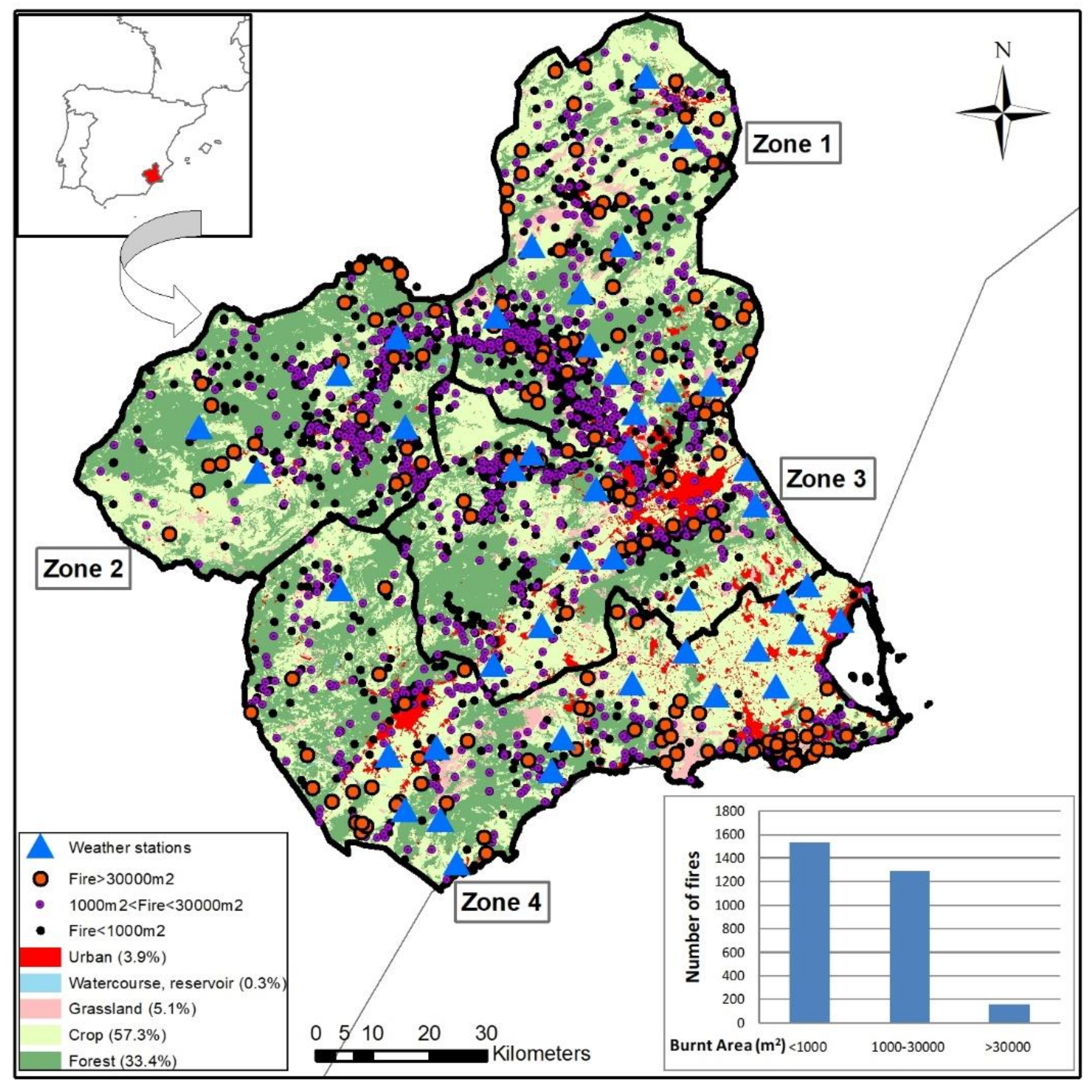
Figure 1. Location of study area, distribution of forest zones, and positions of weather stations and fires according to size of burned area. The histogram shows the relationship between burned area and number of fires.
Applsci 09 04155 g001
Figure 2. Evolution of burned area in ha (bar chart) and Forest Weather Index (FWI) and Angström Index (AI) average on fire days (line chart) in the 2000–2014 period (left and right, respectively).
Applsci 09 04155 g002
Figure 3. General flowchart of the methodology.
Applsci 09 04155 g003
Figure 4. Structure of multilayer perceptron architecture.
Applsci 09 04155 g004
Figure 5. Test matrix of confusion for the 80–20% training-test partition in the study region. Class 1 corresponds to fires smaller than 30,000 m2 (small fires) and class 2 to fires larger than 30,000 m2 (big fires).
Applsci 09 04155 g005
Figure 6. Comparison of average percentage monthly wildfires in recorded period (2000–2014) (blue line) and RCP4.5 (red line) and RCP8.5 (green line) scenarios in long-term period (2070–2100).
Applsci 09 04155 g006
Table 1. Summary of burned area and number of wildfires according the subdivision of zones in the study area (2000–2014).
Zone 1Zone 2Zone 3Zone 4
Area (km2)2928.802378.502439.533564.96
Burned Surface Statistics (m2)Mean632817,099563432,300
Max828,6215,798,460152,0004,181,500
50th percentile697100010002160
75th percentile30004000500010,000
95th percentile20,00020,47925,77289,200
Number of fires<1000 m2676315334210
1000 m2 < A < 30,000 m2443275302275
>30,000 m247242567
Total1166614661552
Burned area (m2)<1000 m2203,07899,92688,07667,090
1000 m2 < A < 30,000 m22,407,9351,586,8321,937,7351,991,938
>30,000 m24,767,1828,811,7481,703,26515,749,205
Total7,378,19510,498,5063,729,07617,808,233
Table 2. Description of input data.
VariableDescription
Xx-axis coordinate UTM ETRS89 30N
Yy-axis coordinate UTM ETRS89 30N
ZAltitude (M.A.S.L.)
MMonth of the year (from 1 to 12)
VegetationType of vegetation in the burned area (from 1 to 3: 1, grassland, 2, forest and 3, crop)
PDaily Rainfall (mm)
HRelative Humidity (%)
TAverage Temperature (°C)
VWind Speed (m/s)
FWIForest Weather Index
AIAngströn Index
Table 3. Final burned-area centroids using k-means algorithm (m2).
Zone 1Zone 2Zone 3Zone 4
k = 53080418421078265
35,21526,59823,28642,568
95,782152,48357,714241,028
259,312710,000107,7741,600,947
455,400992,100152,0004,181,500
k = 436554913235217,169
29,58837,14427,89337,852
187,625711,00075,382160,947
455,40099,200131,0324,181,500
k = 3 36554913239710,258
31,02643,52630,28027,169
211,968851,050105,6182,100,473
Table 4. Confusion matrix of size 2 × 2.
Actual ClassPredicted Class
NegativePositive
Negativeab
Positivecd
Table 5. Comparison of average meteorological data between available historical wildfire data from the period 2000–2014 and future climate change scenarios data (RCP4.5 and RCP8.5) during the period (2071–2100) (Py is average yearly rainfall, H is humidity, T is temperature, and V is wind velocity).
ZonePeriodPy (mm/year)H (%)T (°C)V (m/s)
Zone 12000–2014252.6759.1316.561.06
2071–2100 RCP4.5350.6757.9618.091.24
2071–2100 RCP8.5328.9256.7920.041.21
Zone 22000–2014341.4261.0815.841.96
2071–2100 RCP4.5350.6757.9620.492.49
2071–2100 RCP8.5328.9256.7921.892.43
Zone 32000–2014264.2358.6217.881.39
2071–2100 RCP4.5350.6757.9619.541.75
2071–2100 RCP8.5328.9256.7921.291.69
Zone 42000–2014214.0665.8718.571.79
2071–2100 RCP4.5350.6757.9620.702.08
2071–2100 RCP8.5328.9256.7922.342.04
Table 6. Comparison of historical (2000–2014) and predicted (2071–2100, both RCP4.5 and RCP8.5 scenarios) number of fires in the region.
ZonePeriodTotal Number of FiresAverage Fires Per Year
Zone 12000–201466144.03
2071–2100 RCP4.5198166.00
2071–2100 RCP8.5263287.68
Zone 22000–201461444.90
2071–2100 RCP4.5243781.18
2071–2100 RCP8.53170105.60
Zone 32000–2014116677.68
2071–2100 RCP4.5222274.02
2071–2100 RCP8.5293397.70
Zone 42000–201455236.77
2071–2100 RCP4.5239679.82
2071–2100 RCP8.53177105.83
Table 7. Classification accuracy and values of sensitivity and specificity by the artificial neural network (ANN) classifier for size of wildfire with 50–50%, 60–40%, 70–30%, 80–20%, and 90–10% partitions in training-test, respectively.
ZoneMeasure50–50%60–40%70–30%80–20%90–10%Average
Zone 1Sensitivity (%)57.258.560.963.677.163.46
Specificity (%)62.357.864.170.262.563.38
Accuracy (%)59.158.162.465.970.163.12
Zone 2Sensitivity (%)67.068.365.670.870.068.34
Specificity (%)57.560.769.281.684.670.72
Accuracy (%)61.463.467.475.674.468.44
Zone 3Sensitivity (%)65.562.570.477.475.070.16
Specificity (%)65.158.270.384.171.469.82
Accuracy (%)65.360.370.380.480.071.26
Zone 4Sensitivity (%)48.154.359.460.948.654.26
Specificity (%)69.668.062.564.666.766.28
Accuracy (%)50.258.061.062.853.257.04
Table 8. The 10-fold cross-validation results (%). (SD: standard deviation.).
ZoneK = 1K = 2K = 3K = 4K = 5K = 6K = 7K = 8K = 9K = 10AverageS.D.
Zone 167.653.767.263.270.653.758.852.262.765.761.546.58
Zone 281.476.788.467.474.474.467.481.481.451.274.4110.46
Zone 372.966.779.666.769.462.563.371.456.383.369.218.06
Zone 470.259.655.361.753.268.16661.757.457.461.065.6
Table 9. Goodness-of-fit tests of an ANN (60-20-20 correspond to training, validation, and test, respectively) in prediction of wildfires surface larger than 30,000 m2 in the 2000–2014 period.
ZoneMetricTrainingValidationTest
Zone 1MAE (m2)40,882.3322,644.3239,377.21
RMSE (m2)72,770.1928,197.8379,424.98
MAPE (%)32.5434.1025.88
Bias (m2)37,939.9318,186.42–37,461.56
Zone 2MAE (m2)5643.246060.2328,226.64
RMSE (m2)7353.617087.4134,996.43
MAPE (%)11.7017.2137.38
Bias (m2)–2535.66–5702.80–21,409.82
Zone 3MAE (m2)5695.4918,663.8816,867.68
RMSE (m2)9186.3026,384.2526,047.79
MAPE (%)11.8328.2018.83
Bias (m2)8.8914,958.76–14,095.28
Zone 4MAE (m2)47,778.1914,211.4420,903.01
RMSE (m2)65,997.9417,194.4225,914.53
MAPE (%)42.7729.9240.53
Bias (m2)29,474.66–4890.4018,471.57
Table 10. Comparison of historical (2000–2014) and predicted (2071–2100, both RCP4.5 and RCP8.5 scenarios) burned surface in wildfires larger of 30,000 m2. Increase of total burned surface is related to baseline period 2000–2014.
ZonePeriodTotal Burned Surface (km2)Average Yearly Burned Surface (km2)Increase of Total Burned Surface (%)
Zone 12000–20144.770.32-
2071–2100 RCP4.560.992.03534
2071–2100 RCP8.585.952.86259
Zone 22000–20148.810.59-
2071–2100 RCP4.540.661.36131
2071–2100 RCP8.554.081.80205
Zone 32000–20141.700.11-
2071–2100 RCP4.537.011.231018
2071–2100 RCP8.553.461.781518
Zone 42000–201415.751.05-
2071–2100 RCP4.5118.233.94275
2071–2100 RCP8.5154.055.14390