Gradient Descent-Based Optimization Method of a Four-Bar Mechanism Using Fully Cartesian Coordinates

Abstract

Machine vibrations often occur due to dynamic unbalance inducing wear, fatigue, and noise that limit the potential of many machines. Dynamic balancing is a main concern in mechanism and machine theory as it allows designers to limit the transmission of vibrations to the frames and base of machines. This work introduces a novel method for representing a four-bar mechanism with the use of Fully Cartesian coordinates and a simple definition of the shaking force (ShF) and the shaking moment (ShM) equations. A simplified version of Projected Gradient Descent is used to minimize the ShF and ShM functions with the aim of balancing the system. The multi-objective optimization problem was solved using a linear combination of the objectives. A comprehensive analysis of the partial derivatives, volumes, and relations between area and thickness of the counterweights is used to define whether the allowed optimization boundaries should be changed in case the mechanical conditions of the mechanism permit it. A comparison between Pareto fronts is used to determine the impact that each counterweight has on the mechanism’s balancing. In this way, it is possible to determine which counterweights can be eliminated according to the importance of the static balance (ShF), dynamic balance (ShM), or both. The results of this methodology when using three counterweights reduces the ShF and ShM by 99.70% and 28.69%, respectively when importance is given to the static balancing and by 83.99% and 8.47%, respectively, when importance is focused on dynamic balancing. Even when further reducing the number of counterweights, the ShF and ShM can be decreased satisfactorily.

1. Introduction

A complete mechanical balance or dynamic balance of a mechanism consists of eliminating the dynamic reactions at the base of a mechanism produced by the movement of its structure. These dynamic reactions are the shaking force (ShF) and the shaking moment (ShM). Such balancing is desirable because the ShF and ShM cause vibrations of the supporting frame which latter turn into noise, fatigue, wear, etc. The four-bar mechanism is often taken as example in dynamic balancing because its number of applications [1,2].

Dynamic balancing can be performed in two stages. In the first one, the balancing conditions are commonly obtained using methods that involve Cartesian coordinates and the use of angles; this implies the use of trigonometric functions that derive into complex expressions [3,4,5,6]. In relation to this point, this work exploits the use of fully Cartesian coordinates (also called natural coordinates [7]) to obtain the expressions for optimizing the mechanism balance avoiding any use of angular variables [8,9] and therefore, simplifying the equations. In the second stage, dynamic balancing can be achieved by different methods. A complete review of methods can be found in [3,4,5] and more recently in [6]. All balancing methods imply the addition of masses in some or other form while trying to maintain the total mass as low as possible. Methods based on mass redistribution are very useful from a practical point of view and are very suitable to be implemented. Using optimization techniques, it is possible to minimize the dynamic reactions while maintaining the increment of mass under control. Mass redistribution can be done by optimizing the geometry of the links [10] or by optimizing the size and position of counterweights.

Traditionally, when computational resources were not available, dynamic balancing optimization was carried out using analytic or semi-analytic methods [11,12,13,14,15,16]. Nowadays, technological advances have made it easy to implement advanced numerical optimization techniques. It is usually considered that this kind of formulation is difficult to solve because of the nonlinear nature. The most common technique used to optimize mechanism balancing is meta heuristics. Some examples can be appreciated in [17,18,19]. Herein, techniques like the so-called evolutionary algorithms, Firefly Algorithm, or Differential Evolution, were used, respectively. Some references to methods that transform the objective function to make it convex [20] can also be found. However, they involve a major mathematical analysis.

The optimization algorithm proposed in this paper is a simplified version of Projected Gradient Descent [21], a deterministic and iterative algorithm based on the gradient vector direction. The optimization problem is multi-objective with bound constraints (also known as box constraints). The objective function is obtained by the linear combination of the improvement indexes of the ShF and ShM. This methodology is efficient due to the characteristics of the functions obtained by using fully Cartesian coordinates, allowing to reach a convergence at the minimum value with just few iterations.

This article presents an extension of our previous work [22] in which, with the use of Fully Cartesian coordinates, dynamic balancing optimization of a four-bar mechanism was achieved through the sole addition of counterweights [23,24]. As a novelty, this work presents a comprehensive analysis of the gradient on the optimal points obtained after the first optimization, so it is possible to know whether the proposed limits of the optimized variables can be modified (whenever possible) to obtain even better results than those originally obtained. An analysis of the volume and the relation between the area and the thickness of the counterweights completes and confirms the gradient analysis. The proposed methodology can be used in similar problems to analyze the optimization of mechanisms. In addition, Pareto Fronts are used to present a sensitivity analysis of the response of the whole mechanism when using three, two, or one counterweights. This type of analysis allows to define the importance of each counterweight and determine which ones can be dispensed, obtaining optimum results when trying to optimize the ShF, the ShM, or both.

The rest of the paper is organized as follows: Section 2 presents the mass-matrix definition and calculus of the ShF and ShM equations of a four-bar linkage using fully Cartesian coordinates. Section 3 defines the objective function for the optimization. Section 4 details the algorithm used to optimize the balance and the sensitivity analysis. Section 5 presents the numerical optimization and analysis when using three, two, and one counterweights. Section 6 concludes the paper summarizing the main findings and giving future work perspectives.

2. Mechanical Analysis

2.1. Mass-Matrix of the Four-Bar Linkage Using Fully Cartesian Coordinates

Figure 1 shows a four-bar linkage consisting of four rigid bodies located in the same plane. A motor is located at point A, so the crank AB rotates with velocity $\omega [rads/s]$. $l_{AB},l_{BD}$ and $l_{CD}$ represent the length of each link. By using Fully Cartesian coordinates [9] to represent the system, it is easy to obtain the equations of the ShF and ShM. This method has been previously used in [22,25,26].

To obtain the mass-matrix M of the whole mechanism, it is necessary to define the mass-matrix $M_n$ of each n link. Those matrices can be calculated as presented in [9].

As long as the balance is carried out by adding counterweights, it is necessary to include in M the related parameters. Therefore, each link will be considered as the conjunction of one-bar and one counterweight as shown in Figure 2.

The mass $m_n$ of each link-counterweight $n=1,2,3$ is defined as:

$$\begin{array}{c}\hfill m_n=m_{bn}+m_{cn}\end{array}$$

(1)

where $m_{bn}$ is the mass of the original bar n ($n=1,2,3$) and $m_{cn}$ is the mass of each counterweight ($n=1,2,3$). In addition, the counterweight mass in terms of its density and size can be represented as:

$$\begin{array}{c}\hfill m_{cn}=\pi {\rho }_{cn}{t}_{cn}\left({y_{cn}}^2+{x_{cn}}^2\right)\end{array}$$

(2)

where ${\rho }_{cn}$ is the density of the material used in each counterweight, $t_{cn}$ is the thickness of each counterweight, and $x_{cn},y_{cn}$ represents the position of the center of mass of the counterweight measured in relation with the local coordinate system $O_n$.

The total inertia of each link-counterweight $I_n$, where $n=1,2,3$, is defined as:

$$\begin{array}{c}\hfill I_n=\frac{3m_{cn}\left({y_{cn}}^2+{x_{cn}}^2\right)}{2}+I_{bn}\end{array}$$

(3)

where $x_{cn}$ is the x position of the mass center of the counterweight corresponding to the n element measured from the origin $O_n$ and $y_{cn}$ is the y position of the mass center of the counterweight corresponding to the n element measured from the origin $O_n$. $I_{bn}$ corresponds to the inertia of each original bar.

The new x position of the mass center for each n element is defined as:

$$\begin{array}{c}\hfill X_{Gn}=\frac{m_{cn}{x}_{cn}+m_{bn}{x}_{bn}}{m_{cn}+m_{bn}}\end{array}$$

(4)

And the new y position of the mass center for each n element is defined as:

$$\begin{array}{c}\hfill Y_{Gn}=\frac{m_{cn}{y}_{cn}+m_{bn}{y}_{bn}}{m_{cn}+m_{bn}}\end{array}$$

(5)

where $(x_{cn},y_{cn})$ is the position of the center of mass of each counterweight, and $(x_{bn},y_{bn})$ is the position of the center of mass of each original bar, both measured from the origin $O_n$.

To avoid the use of extra variables, the mass of each counterweight $m_{cn}$ is defined as:

$$m_{cn}=\pi \left(r_{cn}^2\right)\left(t_{cn}\right){\rho }_{cn}$$

(6)

where ${\rho }_{cn}$ represents the density of the counterweight, $t_{cn}$ is the thickness of the counterweight, and $r_{cn}$ represents the ratio of the counterweight.

In addition, if the counterweight is considered to be a cylinder, the radius of the counterweight can be defined as:

$$r_{cn}=\sqrt{x_{cn}^2+y_{cn}^2}$$

(7)

By substituting Equation (7) in (6):

$$m_{cn}=\pi (x_{cn}^2+y_{cn}^2)\left(t_{cn}\right){\rho }_{cn}$$

(8)

and applying the concepts of [9], the mass-matrix representing the whole mechanism can be written as:

$$\mathbf{M}=\left[\begin{array}{cccccccc}a& 0& e& -f& 0& 0& 0& 0\\ 0& a& f& e& 0& 0& 0& 0\\ e& f& b& 0& 0& 0& g& -h\\ -f& e& 0& b& 0& 0& h& g\\ 0& 0& 0& 0& c& 0& i& -j\\ 0& 0& 0& 0& 0& c& j& i\\ 0& 0& g& h& i& j& d& 0\\ 0& 0& -h& g& -j& i& 0& d\end{array}\right]$$

(9)

With:

$$\begin{array}{c}\hfill a=\frac{3\pi {{\rho }_c}_1{t_c}_1{\left({y_c}_1^2+{x_c}_1^2\right)}^2+2{I_b}_1}{2l_1^2}-\frac{2\left(\pi {{\rho }_c}_1{t_c}_1{x_c}_1\left({y_c}_1^2+{x_c}_1^2\right)+{m_b}_1{x_b}_1\right)}{l_1}\\ \hfill +\pi {{\rho }_c}_1{t_c}_1\left({y_c}_1^2+{x_c}_1^2\right)+{m_b}_1\end{array}$$

(10)

$$\begin{array}{c}\hfill b=\frac{3\pi {{\rho }_c}_2{t_c}_2{\left({y_c}_2^2+{x_c}_2^2\right)}^2+2{I_b}_2}{2l_2^2}-\frac{2\left(\pi {{\rho }_c}_2{t_c}_2{x_c}_2\left({y_c}_2^2+{x_c}_2^2\right)+{m_b}_2{x_b}_2\right)}{l_2}\\ \hfill +\pi {{\rho }_c}_2{t_c}_2\left({y_c}_2^2+{x_c}_2^2\right)+{m_b}_2+\frac{3\pi {{\rho }_c}_1{t_c}_1{\left({y_c}_1^2+{x_c}_1^2\right)}^2+2{I_b}_1}{2l_1^2}\end{array}$$

(11)

$$\begin{array}{c}\hfill c=\frac{3\pi {{\rho }_c}_3{t_c}_3{\left({y_c}_3^2+{x_c}_3^2\right)}^2+2{I_b}_3}{2l_3^2}-\frac{2\left(\pi {{\rho }_c}_3{t_c}_3{x_c}_3\left({y_c}_3^2+{x_c}_3^2\right)+{m_b}_3{x_b}_3\right)}{l_3}\\ \hfill +\pi {{\rho }_c}_3{t_c}_3\left({y_c}_3^2+{x_c}_3^2\right)+{m_b}_3\end{array}$$

(12)

$$\begin{array}{c}\hfill d=\frac{3\pi {{\rho }_c}_3{t_c}_3{\left({y_c}_3^2+{x_c}_3^2\right)}^2+2{I_b}_3}{2l_3^2}+\frac{3\pi {{\rho }_c}_2{t_c}_2{\left({y_c}_2^2+{x_c}_2^2\right)}^2+2{I_b}_2}{2l_2^2}\end{array}$$

(13)

$$\begin{array}{c}\hfill e=\frac{\pi {{\rho }_c}_1{t_c}_1{x_c}_1\left({y_c}_1^2+{x_c}_1^2\right)+{m_b}_1{x_b}_1}{l_1}-\frac{3\pi {{\rho }_c}_1{t_c}_1{\left({y_c}_1^2+{x_c}_1^2\right)}^2+2{I_b}_1}{2l_1^2}\end{array}$$

(14)

$$\begin{array}{c}\hfill f=\frac{\pi {{\rho }_c}_1{t_c}_1{y_c}_1\left({y_c}_1^2+{x_c}_1^2\right)+{m_b}_1{y_b}_1}{l_1}\end{array}$$

(15)

$$\begin{array}{c}\hfill g=\frac{\pi {{\rho }_c}_2{t_c}_2{x_c}_2\left({y_c}_2^2+{x_c}_2^2\right)+{m_b}_2{x_b}_2}{l_2}-\frac{3\pi {{\rho }_c}_2{t_c}_2{\left({y_c}_2^2+{x_c}_2^2\right)}^2+2{I_b}_2}{2l_2^2}\end{array}$$

(16)

$$\begin{array}{c}\hfill h=\frac{\pi {{\rho }_c}_2{t_c}_2{y_c}_2\left({y_c}_2^2+{x_c}_2^2\right)+{m_b}_2{y_b}_2}{l_2}\end{array}$$

(17)

$$\begin{array}{c}\hfill i=\frac{\pi {{\rho }_c}_3{t_c}_3{x_c}_3\left({y_c}_3^2+{x_c}_3^2\right)+{m_b}_3{x_b}_3}{l_3}-\frac{3\pi {{\rho }_c}_3{t_c}_3{\left({y_c}_3^2+{x_c}_3^2\right)}^2+2{I_b}_3}{2l_3^2}\end{array}$$

(18)

$$\begin{array}{c}\hfill j=\frac{\pi {{\rho }_c}_3{t_c}_3{y_c}_3\left({y_c}_3^2+{x_c}_3^2\right)+{m_b}_3{y_b}_3}{l_3}\end{array}$$

(19)

2.2. Linear Momentum and Shaking Force

Once the mass-matrix of the whole system is known and based on the basic points of the whole linkage, it is possible to introduce a vector of positions represented by $\mathbf{q}$:

$$\mathbf{q}={\left[\begin{array}{cccccccc}{A}_X& A_Y& B_X& B_Y& C_X& C_Y& D_X& D_Y\end{array}\right]}^{\mathbf{T}}$$

(20)

By time-deriving Equation (20), a vector of velocities can be obtained:

$$\dot{\mathbf{q}}={\left[\begin{array}{cccccccc}{\mathit{VA}}_{\mathit{X}}& {\mathit{VA}}_{\mathit{Y}}& {\mathit{VB}}_{\mathit{X}}& {\mathit{VB}}_{\mathit{Y}}& {\mathit{VC}}_{\mathit{X}}& {\mathit{VC}}_{\mathit{Y}}& {\mathit{VD}}_{\mathit{X}}& {\mathit{VD}}_{\mathit{Y}}\end{array}\right]}^{\mathbf{T}}$$

(21)

By introducing matrix B, it is possible to obtain the linear momentum vectors $\mathbf{L}$ associated to the whole system:

$$\left[\begin{array}{c}{L}_i\\ L_j\end{array}\right]=\mathbf{BM}\dot{\mathbf{q}}$$

(22)

Where B (Equation (23)) is a matrix formed by identity matrices for each of the basic points founded in the mechanism:

$$\mathbf{B}={\left[\begin{array}{cccccccc}1& 0& 1& 0& 1& 0& 1& 0\\ 0& 1& 0& 1& 0& 1& 0& 1\end{array}\right]}^{\mathbf{T}}$$

(23)

By solving Equation (22) and considering the velocity of the fixed points always equal to zero ($V{A}_X=0$, $V{A}_Y=0$, $V{C}_X=0$, $V{C}_Y=0$), the expressions of linear momentum ($L_i$ and $L_j$) for the linkage are obtained.

The shaking force $\mathbf{ShF}$ (Equations (24) and (25)) of the linkage can be calculated from the derivation of Equations $L_i$ and $L_j$ (Equation (22)). To ensure the linkage is force balanced, these equations must be constant (usually zero) over all the analyzed period of time, thus warranting a null shaking force.

$$\begin{array}{c}\hfill Sh{F}_i=\frac{d{L}_i}{dt}=\left(-\frac{\pi {{\rho }_c}_3{t_c}_3{y_c}_3\left({y_c}_3^2+{x_c}_3^2\right)+{m_b}_3{y_b}_3}{l_3}-\frac{\pi {{\rho }_c}_2{t_c}_2{y_c}_2\left({y_c}_2^2+{x_c}_2^2\right)+{m_b}_2{y_b}_2}{l_2}\right){\mathit{AD}}_Y\\ \hfill +\left(\frac{\pi {{\rho }_c}_3{t_c}_3{x_c}_3\left({y_c}_3^2+{x_c}_3^2\right)+{m_b}_3{x_b}_3}{l_3}+\frac{\pi {{\rho }_c}_2{t_c}_2{x_c}_2\left({y_c}_2^2+{x_c}_2^2\right)+{m_b}_2{x_b}_2}{l_2}\right){\mathit{AD}}_X\\ \hfill +\frac{\left(\pi {{\rho }_c}_3{t_c}_3{y_c}_3\left({y_c}_3^2+{x_c}_3^2\right)+{m_b}_3{y_b}_3\right){\mathit{AC}}_Y}{l_3}\\ \hfill +\left(-\frac{\pi {{\rho }_c}_3{t_c}_3{x_c}_3\left({y_c}_3^2+{x_c}_3^2\right)+{m_b}_3{x_b}_3}{l_3}+\pi {{\rho }_c}_3{t_c}_3\left({y_c}_3^2+{x_c}_3^2\right)+{m_b}_3\right){\mathit{AC}}_X\\ \hfill +\left(\frac{\pi {{\rho }_c}_2{t_c}_2{y_c}_2\left({y_c}_2^2+{x_c}_2^2\right)+{m_b}_2{y_b}_2}{l_2}-\frac{\pi {{\rho }_c}_1{t_c}_1{y_c}_1\left({y_c}_1^2+{x_c}_1^2\right)+{m_b}_1{y_b}_1}{l_1}\right){\mathit{AB}}_Y\\ \hfill +(-\frac{\pi {{\rho }_c}_2{t_c}_2{x_c}_2\left({y_c}_2^2+{x_c}_2^2\right)+{m_b}_2{x_b}_2}{l_2}+\pi {{\rho }_c}_2{t_c}_2\left({y_c}_2^2+{x_c}_2^2\right)\\ \hfill +{m_b}_2+\frac{\pi {{\rho }_c}_1{t_c}_1{x_c}_1\left({y_c}_1^2+{x_c}_1^2\right)+{m_b}_1{x_b}_1}{l_1}){\mathit{AB}}_X\\ \hfill +\frac{\left(\pi {{\rho }_c}_1{t_c}_1{y_c}_1\left({y_c}_1^2+{x_c}_1^2\right)+{m_b}_1{y_b}_1\right){\mathit{AA}}_Y}{l_1}\\ \hfill +\left(-\frac{\pi {{\rho }_c}_1{t_c}_1{x_c}_1\left({y_c}_1^2+{x_c}_1^2\right)+{m_b}_1{x_b}_1}{l_1}+\pi {{\rho }_c}_1{t_c}_1\left({y_c}_1^2+{x_c}_1^2\right)+{m_b}_1\right){\mathit{AA}}_X\end{array}$$

(24)

$$\begin{array}{c}\hfill Sh{F}_j=\frac{d{L}_j}{dt}=\left(\frac{\pi {{\rho }_c}_3{t_c}_3{x_c}_3\left({y_c}_3^2+{x_c}_3^2\right)+{m_b}_3{x_b}_3}{l_3}+\frac{\pi {{\rho }_c}_2{t_c}_2{x_c}_2\left({y_c}_2^2+{x_c}_2^2\right)+{m_b}_2{x_b}_2}{l_2}\right){\mathit{AD}}_Y\\ \hfill +\left(\frac{\pi {{\rho }_c}_3{t_c}_3{y_c}_3\left({y_c}_3^2+{x_c}_3^2\right)+{m_b}_3{y_b}_3}{l_3}+\frac{\pi {{\rho }_c}_2{t_c}_2{y_c}_2\left({y_c}_2^2+{x_c}_2^2\right)+{m_b}_2{y_b}_2}{l_2}\right){\mathit{AD}}_X\\ \hfill +\left(-\frac{\pi {{\rho }_c}_3{t_c}_3{x_c}_3\left({y_c}_3^2+{x_c}_3^2\right)+{m_b}_3{x_b}_3}{l_3}+\pi {{\rho }_c}_3{t_c}_3\left({y_c}_3^2+{x_c}_3^2\right)+{m_b}_3\right){\mathit{AC}}_Y\\ \hfill -\frac{\left(\pi {{\rho }_c}_3{t_c}_3{y_c}_3\left({y_c}_3^2+{x_c}_3^2\right)+{m_b}_3{y_b}_3\right){\mathit{AC}}_X}{l_3}\\ \hfill +(-\frac{\pi {{\rho }_c}_2{t_c}_2{x_c}_2\left({y_c}_2^2+{x_c}_2^2\right)+{m_b}_2{x_b}_2}{l_2}+\pi {{\rho }_c}_2{t_c}_2\left({y_c}_2^2+{x_c}_2^2\right)\\ \hfill +{m_b}_2+\frac{\pi {{\rho }_c}_1{t_c}_1{x_c}_1\left({y_c}_1^2+{x_c}_1^2\right)+{m_b}_1{x_b}_1}{l_1}){\mathit{AB}}_Y\\ \hfill +\left(\frac{\pi {{\rho }_c}_1{t_c}_1{y_c}_1\left({y_c}_1^2+{x_c}_1^2\right)+{m_b}_1{y_b}_1}{l_1}-\frac{\pi {{\rho }_c}_2{t_c}_2{y_c}_2\left({y_c}_2^2+{x_c}_2^2\right)+{m_b}_2{y_b}_2}{l_2}\right){\mathit{AB}}_X\\ \hfill +\left(-\frac{\pi {{\rho }_c}_1{t_c}_1{x_c}_1\left({y_c}_1^2+{x_c}_1^2\right)+{m_b}_1{x_b}_1}{l_1}+\pi {{\rho }_c}_1{t_c}_1\left({y_c}_1^2+{x_c}_1^2\right)+{m_b}_1\right){\mathit{AA}}_Y\\ \hfill -\frac{\left(\pi {{\rho }_c}_1{t_c}_1{y_c}_1\left({y_c}_1^2+{x_c}_1^2\right)+{m_b}_1{y_b}_1\right){\mathit{AA}}_X}{l_1}\end{array}$$

(25)

2.3. Angular Momentum and Shaking Moment

The use of Fully Cartesian coordinates allows to express the angular momentum H as Equation (26) with $\mathbf{r}$ defined as shown in Equation (27).

$$H=\mathbf{q}\times \left(\mathbf{M}\dot{\mathbf{q}}\right)=\mathbf{rM}\dot{\mathbf{q}}$$

(26)

$$\mathbf{r}={\left[\begin{array}{cccccccc}-A_Y& A_X& -B_Y& B_X& -C_Y& C_X& -D_Y& D_X\end{array}\right]}^{\mathbf{T}}$$

(27)

By solving Equation (26) and considering ${\mathit{VA}}_{\mathit{X}}=\mathit{0}$, ${\mathit{VA}}_{\mathit{Y}}=\mathit{0}$, ${\mathit{VC}}_{\mathit{X}}=\mathit{0}$ and ${\mathit{VC}}_{\mathit{Y}}=\mathit{0}$, the expression of the angular momentum H can be obtained.

A scalar value corresponding to the shaking moment $ShM$ of the linkage that is considered perpendicular to the plane of the 2D mechanism, can be calculated by time-deriving H:

$$\begin{array}{c}\hfill ShM=\frac{dH}{dt}=\mathbf{rM}\left(\frac{d\left(\dot{\mathbf{q}}\right)}{dt}\right)+\left(\frac{d\mathbf{r}}{dt}\right)\mathbf{M}\dot{\mathbf{q}}\end{array}$$

(28)

$$\begin{array}{c}\hfill ShM=\frac{dH}{dt}=\mathbf{rM}\ddot{\mathbf{q}}+\dot{\mathbf{r}}\mathbf{M}\dot{\mathbf{q}}\end{array}$$

(29)

where:

$$\dot{\mathbf{r}}={[-{VA}_Y{VA}_X-{VB}_Y{VB}_X-{VC}_Y{VC}_X-{VD}_Y{VD}_X]}^{\mathbf{T}}$$

(30)

and $\ddot{\mathbf{q}}$, the time-derivation of vector $\dot{\mathbf{q}}$, represents the acceleration vector.

To guarantee the dynamic balancing of the mechanism, $ShM$ must be kept constant: The time-derivation of H (Equations (28) and (29)) should be zero.

By solving Equation (29) and considering ${\mathit{VA}}_{\mathit{X}}=\mathit{0}$, ${\mathit{VA}}_{\mathit{Y}}=\mathit{0}$, ${\mathit{VC}}_{\mathit{X}}=\mathit{0}$ and ${\mathit{VC}}_{\mathit{Y}}=\mathit{0}$, the $ShM$ of the four-bar linkage can be obtained:

$$\begin{array}{c}\hfill ShM={\mathit{VD}}_X\left(\left(\frac{3\pi {{\rho }_c}_3{t_c}_3{\left({y_c}_3^2+{x_c}_3^2\right)}^2+{2I_b}_3}{2l_3^2}+\frac{3\pi {{\rho }_c}_2{t_c}_2{\left({y_c}_2^2+{x_c}_2^2\right)}^2+2{I_b}_2}{2l_2^2}\right){\mathit{VD}}_Y\right.\\ \hfill +\left(\frac{\pi {{\rho }_c}_2{t_c}_2{x_c}_2\left({y_c}_2^2+{x_c}_2^2\right)+{m_b}_2{x_b}_2}{l_2}-\frac{3\pi {{\rho }_c}_2{t_c}_2{\left({y_c}_2^2+{x_c}_2^2\right)}^2+2{I_b}_2}{2l_2^2}\right){\mathit{VB}}_Y\\ \hfill \left.-\frac{\left(\pi {{\rho }_c}_2{t_c}_2{y_c}_2\left({y_c}_2^2+{x_c}_2^2\right)+{m_b}_2{y_b}_2\right){\mathit{VB}}_X}{l_2}\right)+{\mathit{VB}}_X-{\mathit{VB}}_Y\\ \hfill -\left(\frac{3\pi {{\rho }_c}_3{t_c}_3{\left({y_c}_3^2+{x_c}_3^2\right)}^2+2{I_b}_3}{2l_3^2}+\frac{3\pi {{\rho }_c}_2{t_c}_2{\left({y_c}_2^2+{x_c}_2^2\right)}^2+2{I_b}_2}{2l_2^2}\right){\mathit{VD}}_X{\mathit{VD}}_Y\\ \hfill -\frac{\left(\pi {{\rho }_c}_2{t_c}_2{y_c}_2\left({y_c}_2^2+{x_c}_2^2\right)+{m_b}_2{y_b}_2\right){\mathit{VB}}_Y{\mathit{VD}}_Y}{l_2}\\ \hfill -\left(\frac{\pi {{\rho }_c}_2{t_c}_2{x_c}_2\left({y_c}_2^2+{x_c}_2^2\right)+{m_b}_2{x_b}_2}{l_2}-\frac{3\pi {{\rho }_c}_2{t_c}_2{\left({y_c}_2^2+{x_c}_2^2\right)}^2+2{I_b}_2}{2l_2^2}\right){\mathit{VB}}_X{\mathit{VD}}_Y\\ \hfill -\left(\left(\frac{3\pi {{\rho }_c}_3{t_c}_3{\left({y_c}_3^2+{x_c}_3^2\right)}^2+2{I_b}_3}{2l_3^2}+\frac{3\pi {{\rho }_c}_2{t_c}_2{\left({y_c}_2^2+{x_c}_2^2\right)}^2+2{I_b}_2}{2l_2^2}\right){\mathit{AD}}_X\right.\\ \hfill +\frac{\left(\pi {{\rho }_c}_2{t_c}_2{y_c}_2\left({y_c}_2^2+{x_c}_2^2\right)+{m_b}_2{y_b}_2\right){\mathit{AB}}_Y}{l_2}\\ \hfill \left.+\left(\frac{\pi {{\rho }_c}_2{t_c}_2{x_c}_2\left({y_c}_2^2+{x_c}_2^2\right)+{m_b}_2{x_b}_2}{l_2}-\frac{3\pi {{\rho }_c}_2{t_c}_2{\left({y_c}_2^2+{x_c}_2^2\right)}^2+2{I_b}_2}{2l_2^2}\right){\mathit{AB}}_X\right)D_Y\\ \hfill +\left(\left(\frac{3\pi {{\rho }_c}_3{t_c}_3{\left({y_c}_3^2+{x_c}_3^2\right)}^2+2{I_b}_3}{2l_3^2}+\frac{3\pi {{\rho }_c}_2{t_c}_2{\left({y_c}_2^2+{x_c}_2^2\right)}^2+2{I_b}_2}{2l_2^2}\right){\mathit{AD}}_Y\right.\\ \hfill +\left(\frac{\pi {{\rho }_c}_2{t_c}_2{x_c}_2\left({y_c}_2^2+{x_c}_2^2\right)+{m_b}_2{x_b}_2}{l_2}-\frac{3\pi {{\rho }_c}_2{t_c}_2{\left({y_c}_2^2+{x_c}_2^2\right)}^2+2{I_b}_2}{2l_2^2}\right){\mathit{AB}}_Y\\ \hfill \left.-\frac{\left(\pi {{\rho }_c}_2{t_c}_2{y_c}_2\left({y_c}_2^2+{x_c}_2^2\right)+{m_b}_2{y_b}_2\right){\mathit{AB}}_X}{l_2}\right)D_X\\ \hfill +\left(\left(\frac{\pi {{\rho }_c}_3{t_c}_3{x_c}_3\left({y_c}_3^2+{x_c}_3^2\right)+{m_b}_3{x_b}_3}{l_3}-\frac{3\pi {{\rho }_c}_3{t_c}_3{\left({y_c}_3^2+{x_c}_3^2\right)}^2+2{I_b}_3}{2l_3^2}\right){\mathit{AD}}_Y\right.\\ \hfill \left.+\frac{\left(\pi {{\rho }_c}_3{t_c}_3{y_c}_3\left({y_c}_3^2+{x_c}_3^2\right)+{m_b}_3{y_b}_3\right){\mathit{AD}}_X}{l_3}\right)C_X-B_Y+B_X\end{array}$$

(31)

3. Objective Function

A dimensionless balancing index ${\beta }_i$ can be used to define the optimization’s objective function. This kind of expressions has been previously used in [14,24], and more recently in [20]. As shown in Equation (32), the first balancing index is defined by the relation of the root mean square (rms) of the reaction of the optimized linkage ($rms{(}^{o}Reaction)$) with respect to the rms value of the reaction of the original linkage ($rms\left(Reaction\right)$), both considered over a period of time T.

Two objective indexes will be considered taking in account the reactions of the ShF and ShM. As long as they represent the ratio between the reactions of the original mechanism and the optimized one, the result will present the achieved optimization. The value is in the range (0, 1). The nearest this value is to 0, the best balance is achieved. Otherwise (a value close to 1), the result is almost the same that the one obtained without balancing.

The first balancing index ${\beta }_{ShF}$ is shown in Equation (32).

$${\beta }_{ShF}=\frac{rms{(}^{o}ShF)}{rms\left(ShF\right)}$$

(32)

where the root mean square of the ShF ($rms\left(ShF\right)$) is given by:

$$rms\left(ShF\right)=\sqrt{\frac{1}{N}\sum _{k=1}^N(Sh{F}_{ik}^2+Sh{F}_{jk}^2)}$$

(33)

and the root mean square of the original ShF ($rms{(}^{o}ShF)$) is a constant value obtained from calculating the root mean square of the ShF of the four-bar linkage without any added counterweight.

$$rms{(}^{o}ShF)=\sqrt{\frac{1}{N}\sum _{k=1}^N{(}^{o}Sh{F}_{ik}^2{+}^{o}Sh{F}_{jk}^2)}$$

(34)

By substituting Equations (33) and (34) in Equation (32), the balancing index (${\beta }_{ShF}$) can be expressed as:

$${\beta }_{ShF}=\sqrt{\frac{{\sum }_{k=1}^N(Sh{F}_{ik}^2+Sh{F}_{jk}^2)}{{\sum }_{k=1}^N{(}^{o}Sh{F}_{ik}^2{+}^{o}Sh{F}_{jk}^2)}}$$

(35)

Similarly, the second objective index can be calculated when the ShM is considered as the reaction. So, ${\beta }_{ShM}$ can be written as:

$${\beta }_{ShM}=\sqrt{\frac{{\sum }_{k=1}^{N}Sh{M}_k^2}{{\sum }_{k=1}^N{}^{o}Sh{M}_k^2}}$$

(36)

where $ShM$ is the shaking moment of the optimized linkage when using the added counterweights and ${}^{o}ShM$ is a constant value that represents the shaking moment of the unbalanced linkage.

The optimization objective is to minimize ${\beta }_{ShF}$ and ${\beta }_{ShM}$ considering boundary limits while ensuring that the coordinates of the centers of mass ($x_{cn}$ and $y_{cn}$) and the thickness ($t_{cn}$) of each counterweight are dimensions that can be used in the mechanical context. Therefore, the boundaries for optimization are limited according to:

$$x_{cn}^{min}⩽x_{cn}⩽x_{cn}^{max}$$

(37)

$$y_{cn}^{min}⩽y_{cn}⩽y_{cn}^{max}$$

(38)

$$t_{cn}^{min}⩽t_{cn}⩽t_{cn}^{max}$$

(39)

4. Optimization

The optimization theory deals with selecting the best alternative in the sense of the given objective function [27]. It can be applied to solve a wide variety of problems, for example: [28,29,30].

Mathematically, optimization is the process of finding the minimum or the maximum of a function $f\left(\mathbf{X}\right):{\mathbb{R}}^n->\mathbb{R}$. $\mathbf{X}\in {\mathbb{R}}^n$ is the vector of variables that can be modified in order to optimize $f\left(\mathbf{X}\right)$. When minimizing the function f, an optimal solution can be defined as ${\mathbf{X}}^{*}$ where $f\left({\mathbf{X}}^{*}\right)\le f\left(\mathbf{X}\right)$ for all $\mathbf{X}\in {\mathbb{R}}^n$. In other words, it is a global minimum.

4.1. Simplified Version of the Projected Gradient Descent

Gradient Descent is an iterative algorithm that finds a local minimal in a function [21,27,28]. It starts in a random point and continues until the minimal is reached. This technique is based on the use of the gradient vector to update the solution. The gradient vector $\nabla \mathbf{f}\left(\mathbf{X}\right)$ evaluated in a point X points the direction of a maximum ascent. Gradient Descent moves the point in the opposite direction to the gradient. The problem starts with the solution vector $X_0$ and in each iteration ${\mathbf{X}}_{\mathbf{k}}$ is modified according to Equation (40).

$${\mathbf{X}}_{\mathbf{k}+\mathbf{1}}={\mathbf{X}}_{\mathbf{k}}+{\alpha }_k{\mathbf{P}}_{\mathbf{k}}$$

(40)

where k is the current iteration, ${\alpha }_k$ is the step length, and ${\mathbf{P}}_{\mathbf{k}}$ is the direction calculated as an unitary direction vector as shown in Equation (41).

$${\mathbf{P}}_{\mathbf{k}}=-\frac{\nabla \mathbf{f}\left({\mathbf{X}}_{\mathbf{k}}\right)}{\left|\right|\nabla \mathbf{f}\left({\mathbf{X}}_{\mathbf{k}}\right)\left|\right|}$$

(41)

The step length ${\alpha }_k$ is optimized based on the approximation of the Taylor’s Theorem (Equation (42)), ensuring this way the maximum descent.

$$f({\mathbf{X}}_{\mathbf{k}}+{\alpha }_k{\mathbf{P}}_{\mathbf{k}})\approx f\left({\mathbf{X}}_{\mathbf{k}}\right)+{\alpha }_k{{\mathbf{P}}_{\mathbf{k}}}^T\nabla \mathbf{f}\left({\mathbf{X}}_{\mathbf{k}}\right)+\frac{{\alpha }_k^2}{2}{{\mathbf{P}}_{\mathbf{k}}}^T{\nabla }^{\mathbf{2}}\mathbf{f}\left({\mathbf{X}}_{\mathbf{k}}\right){\mathbf{P}}_{\mathbf{k}}$$

(42)

By deriving Equation (42) with respect to $\alpha$ and clearing $\alpha$:

$${\alpha }_k=-\frac{{\nabla \mathbf{f}\left(\mathbf{X}\right)}^T{\mathbf{P}}_{\mathbf{k}}}{{{\mathbf{P}}_{\mathbf{k}}}^T{\nabla }^{\mathbf{2}}\mathbf{f}\left(\mathbf{X}\right){\mathbf{P}}_{\mathbf{k}}}$$

(43)

4.2. Finite Difference

Calculating the derivatives in a symbolic way may be difficult on certain occasions. Finite Differences [21] can be used to obtain an approximation of the Gradient Vector and the Hessian matrix.

Mathematically, the Gradient vector $\nabla \mathbf{f}\left(\mathbf{X}\right)$ is formed by the first derivatives of the function with respect to all the variables (Equation (44)) and the Hessian matrix ${\nabla }^{\mathbf{2}}\mathbf{f}\left(\mathbf{X}\right)$ is composed of the second derivatives (Equation (45)).

$$\nabla \mathbf{f}\left(\mathbf{X}\right)={\left[\begin{array}{cccc}\frac{\partial f}{\partial x_1},& \frac{\partial f}{\partial x_2},& \cdots ,& \frac{\partial f}{\partial x_n}\end{array}\right]}^T$$

(44)

$${\nabla }^{\mathbf{2}}\mathbf{f}\left(\mathbf{X}\right)=\left[\begin{array}{cccc}\frac{{\partial }^{2}f}{\partial x_1^2}& \frac{{\partial }^{2}f}{\partial x_1\partial x_2}& \cdots & \frac{{\partial }^{2}f}{\partial x_1\partial x_n}\\ \frac{{\partial }^{2}f}{\partial x_2\partial x_1}& \frac{{\partial }^{2}f}{\partial x_2^2}& \cdots & \frac{{\partial }^{2}f}{\partial x_2\partial x_n}\\ ⋮& ⋮& \ddots & ⋮\\ \frac{{\partial }^{2}f}{\partial x_{\mathrm{n}}\partial x_1}& \frac{{\partial }^{2}f}{\partial x_{\mathrm{n}}\partial x_2}& ⋮& \frac{{\partial }^{2}f}{\partial x_{\mathrm{n}}^2}\end{array}\right]$$

(45)

To approximate the first partial derivatives, Equation (46) is used. Here, $ϵ$ is a scalar constant with a small value ($ϵ=1e-5$), ${\mathbf{e}}_{\mathbf{i}}$ is a unitary vector with the size of $\mathbf{X}$ that contains 0’s in all its positions except in the position i where there is a 1.

$$\frac{\partial f}{\partial X_i}=\frac{f(\mathbf{X}+ϵ{\mathbf{e}}_{\mathbf{i}})-f\left(\mathbf{X}\right)}{ϵ}$$

(46)

Since the Hessian matrix will be multiplied by a vector, a finite approximation is used (Equation (47)), where V is the vector to be multiplied.

$${\nabla }^{\mathbf{2}}\mathbf{f}\left(\mathbf{X}\right)\ast \mathbf{V}=\frac{\nabla \mathbf{f}(\mathbf{X}+ϵ\mathbf{V})-\nabla \mathbf{f}\left(\mathbf{X}\right)}{ϵ}$$

(47)

4.3. Implementation to Optimize the ShF and ShM

The optimization problem consists of minimizing ${\beta }_{ShF}$ and ${\beta }_{ShM}$ (see Equations (35) and (36)). $\mathbf{X}$ is the vector that contains all the variables values that need to be calculated, this is, $\mathbf{X}=[x_{c1},y_{c1},t_{c1},x_{c2},y_{c2},t_{c2},x_{c3},y_{c3},t_{c3}]$. As two functions need to be optimized, ${\beta }_{ShF}$ and ${\beta }_{ShM}$, it can be stated that this is a multi-objective problem. In this research, the objectives are in conflict, it means that, when optimizing the values of $\mathbf{X}$ for minimizing ${\beta }_{ShF}$, a worse value of ${\beta }_{ShM}$ can be obtained and vice-versa. 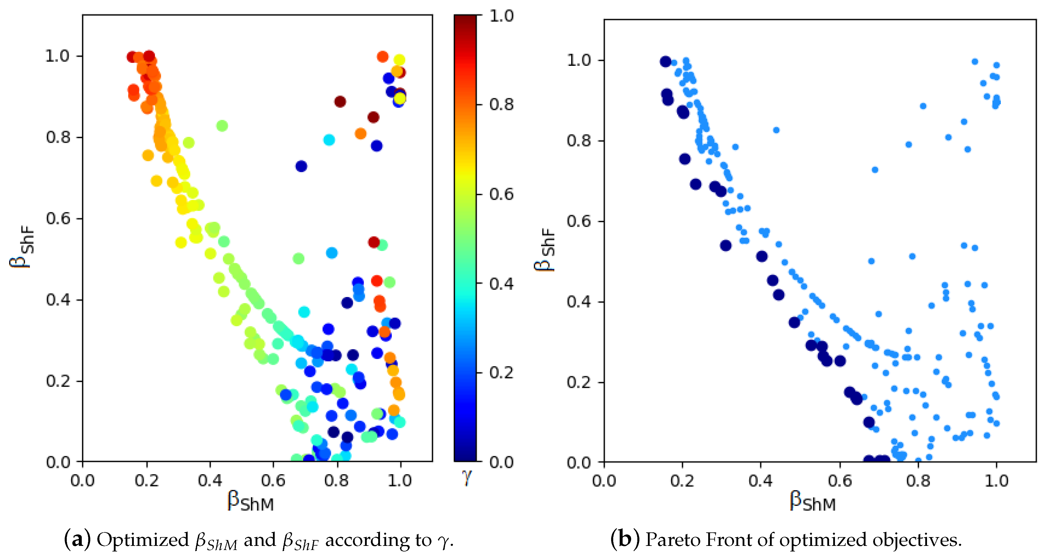All the solutions $\mathbf{X}$ can be represented in a two dimensional plane with the pair $({\beta }_{ShF}\left(\mathbf{X}\right),{\beta }_{ShM}\left(\mathbf{X}\right))$, as it can be seen in Figure 4. We say a solution is dominated ${\mathbf{X}}^{\mathbf{d}}$ when its two objectives are worse than at least other solution, this is, $\exists x:{\beta }_{ShF}\left({\mathbf{X}}^{\mathbf{d}}\right)\ge {\beta }_{ShF}\left(\mathbf{X}\right)\wedge {\beta }_{ShF}\left({\mathbf{X}}^{\mathbf{d}}\right)\ge {\beta }_{ShF}\left(\mathbf{X}\right)$. And the non-dominated solutions ${\mathbf{X}}^{*}$ are the ones that ${\beta }_{ShF}\left({\mathbf{X}}^{*}\right)\le {\beta }_{ShF}\left(\mathbf{X}\right)\vee {\beta }_{ShM}\left({\mathbf{X}}^{*}\right)\le {\beta }_{ShM}\left(\mathbf{X}\right)\forall x$. Figure 4b shows an example of non-dominated (dark blue) and dominated solutions (light blue). The Pareto Front [17] is conformed by the non-dominated solutions. According to the specific mechanical reaction that is more urgent to optimize, it is recommended to choose a specific solution from the Pareto Frontier.

The technique weighted sum [31], that is widely known for solving multi-objective problems, was used for defining the objective function of the optimization problem (Equation (48)).

$$f\left(\mathbf{X}\right)=\gamma \ast {\beta }_{ShM}\left(\mathbf{X}\right)+(1-\gamma )\ast {\beta }_{ShF}\left(\mathbf{X}\right)$$

(48)

where $\gamma$ is a scalar value that determines the importance given to each of the objectives of the optimization.

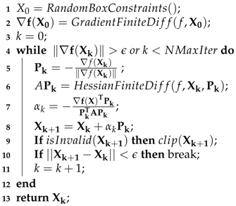
The simplified version of Projected Gradient Descent algorithm is used for solving the optimization problem (Equation (48)). It is described in Algorithm 1. $RandomBoxConstraints\left(\right)$ calculates a vector of random variables with uniform distribution respecting the specified bounds. $GradientFiniteDiff(f,{\mathbf{X}}_{\mathbf{0}})$ and $HessianFiniteDiff(f,{\mathbf{X}}_{\mathbf{k}},{\mathbf{P}}_{\mathbf{k}})$ calculate the approximation of the Gradient vector and the Hessian matrix based on the Equations (44), (46) and (47). $∥.∥$ represents the vector norm. $ϵ$ is a small scalar ($ϵ=1e-5$).

To handle bound constraints, a simplified version of Projected Gradient Descent is used, so when a solution is found outside of the boundaries, it is projected to the valid region. The Boolean function $isInvalid\left({\mathbf{X}}_{\mathbf{k}+\mathbf{1}}\right)$ returns true if the obtained vector contains values inside the boundaries otherwise, it returns false. The function $clip\left({\mathbf{X}}_{\mathbf{k}+\mathbf{1}}\right)$ is used to clip the values of the vector if they are not valid. Clipping the values implies that if the value is smaller than the lower value allowed, then the value is converted to the minimal. In the same way, if the value is bigger than the maximum value allowed, then the value is converted to the maximum.

The algorithm implements two stop conditions: (1) $\left|\right|{\mathbf{X}}_{\mathbf{k}+\mathbf{1}}-{\mathbf{X}}_{\mathbf{k}}\left|\right|<ϵ$. It means that the difference between ${\mathbf{X}}_{\mathbf{k}+\mathbf{1}}$ and ${\mathbf{X}}_{\mathbf{k}}$ is too small, so there is no change in the current solution, this also includes when the Gradient vector norm is close to 0. (2) $k>NMaxIter$. It means that the maximum number of iterations has been reached (In this work $NMaxIter=1000)$.

Algorithm 1: Projected Gradient Descent with maximum descent.

The objective function defined in Equation (48) is non convex, therefore it has different local minimums. For this reason, the algorithm 1 is executed 500 times, each one with a different starting point with the goal of finding the different local minimums. Based on a random search for hyperparameters presented in [32], $\gamma$ is taken as a random value from a uniform distribution in the range $(0,1)$ (see Equation (48)). When the optimization objective values are less than 1.0, the resultant parameters are stored.

4.4. Sensibility Analysis

This subsection shows a way to analyze the Gradient vector values and the constraints.

The optimization problem can be defined as:

$$\begin{array}{c}\underset{\mathbf{X}}{min}f(\mathbf{X},\alpha )\\ & s.t.\\ & \mathbf{l}<=\mathbf{X}<=\mathbf{h}\end{array}$$

(49)

And the constraints can be redefined as:

$$\begin{array}{c}\underset{\mathbf{X}}{min}f(\mathbf{X},\alpha )\\ & s.t.\\ & \mathbf{X}-\mathbf{l}>=0\\ & \mathbf{h}-\mathbf{X}>=0\end{array}$$

(50)

In this case, the Lagrangian is given by:

$$L(\mathbf{X},\delta ,\pi )=f\left(\mathbf{X}\right)-{\delta }^T\left(\mathbf{l}\right)-{\pi }^T(\mathbf{h}-\mathbf{X})$$

(51)

and the KKT:

$$\nabla \mathbf{f}\left(\mathbf{X}\right)-\delta +\pi =0$$

(52)

with $\delta ,\pi >=0$, defining $\lambda =\delta -\pi$

$$\nabla \mathbf{f}\left(\mathbf{X}\right)-\lambda =0$$

(53)

$$\nabla \mathbf{f}\left(\mathbf{X}\right)=\lambda$$

(54)

Then

$${\delta }_i=\left\{\begin{array}{ccc}0& if& {\lambda }_i=0\\ {\lambda }_i& if& {\lambda }_i>0\\ 0& if& {\lambda }_i<0\end{array}\right.$$

(55)

$${\pi }_i=\left\{\begin{array}{ccc}0& if& {\lambda }_i=0\\ 0& if& {\lambda }_i>0\\ -{\lambda }_i& if& {\lambda }_i<0\end{array}\right.$$

(56)

In other words, if the $i-th$ entry of the Gradient has a value equal to 0, the constraint is not affected. If the value is greater than 0, the constraint of the lower border is affected. Finally, if the value is smaller than 0, the constraint of the higher border is affected.

5. Analysis

This section presents a deep analysis that provides information on the importance of each counterweight and its influence on the balance of the mechanism. It also presents a method to determinate if the optimization limits are the most appropriate or if it is convenient to change them in case the mechanical limitations of the system allows it.

5.1. Using Three Counterweights

5.1.1. Mechanical Characteristics

Table 1. Parameters of the four-bar mechanism used in the example.

Body n	1	2	3
Mass $m_{b_n}$ [kg]	2.51946901	4.73866901	3.68746901
Lenght $l_n$ [m]	0.40	0.78	0.60
Inertia $I_{b_n}$ $\left[\mathrm{kg}{\mathrm{m}/\mathrm{s}}^2\right]$	0.14023528	0.98146460	0.45494271
Center of mass $x_{b_n}$ [m]	0.20	0.39	0.30
Center of mass $y_{b_n}$ [m]	0.00	0.00	0.00

presents the parameters of a four-bar linkage (Figure 2). The material used for the links is steel with a density of 7800 kg/m${}^3$. The counterweights are made from brass with a density (${\rho }_c$) of 8500 kg/m${}^3$.

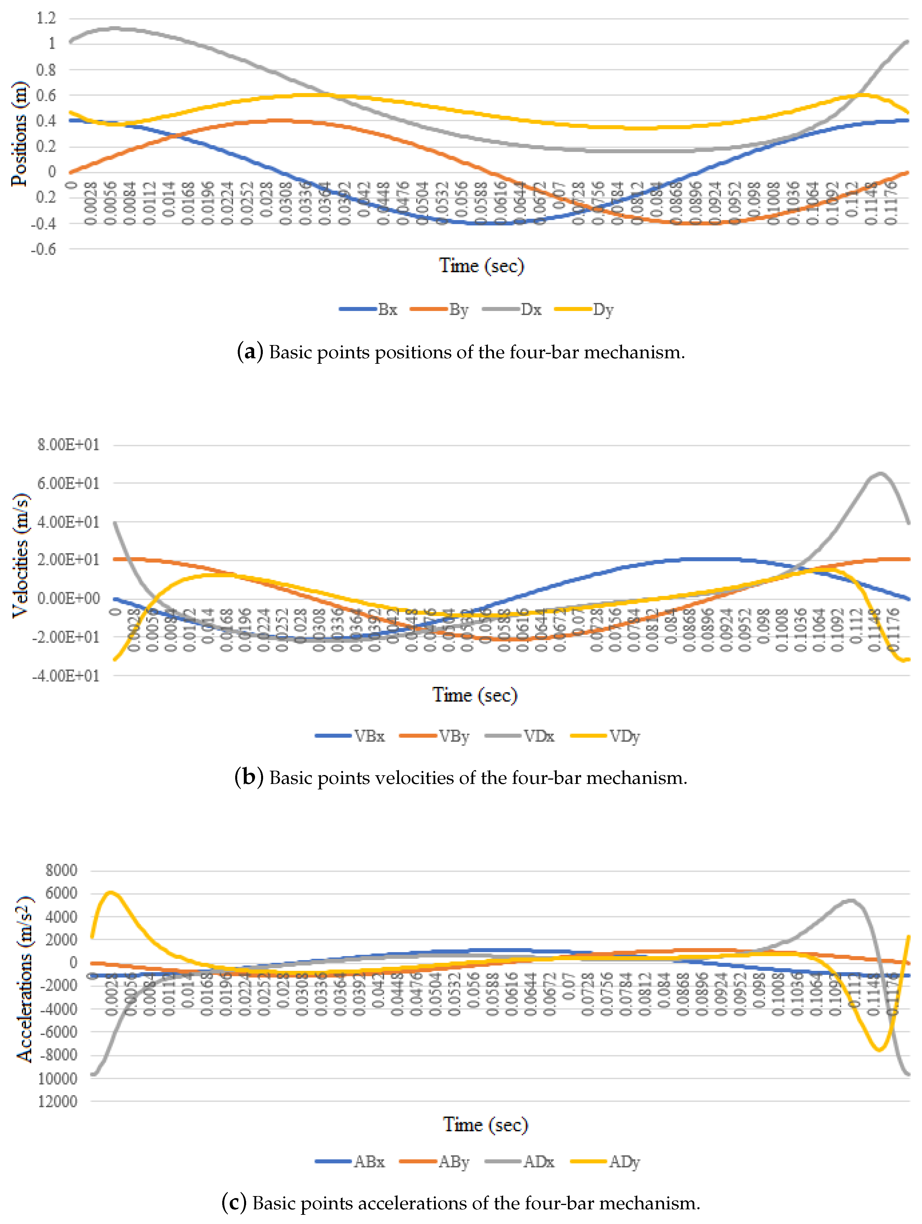
The mechanism is moved by a motor placed at point A, rotating at a constant speed of 500 rpm. Using direct kinematics, it is possible to obtain a sample of the positions ($A_x$, $A_y$, $B_x$, $B_y$, $C_x$, $C_y$,$D_x$, $D_y$), speeds (${\mathit{VB}}_{\mathit{x}}$, ${\mathit{VB}}_{\mathit{y}}$, ${\mathit{VC}}_{\mathit{x}}$, ${\mathit{VC}}_{\mathit{y}}$, ${\mathit{VD}}_{\mathit{x}}$, ${\mathit{VD}}_{\mathit{y}}$) and accelerations ${\mathit{AB}}_{\mathit{x}}$, ${\mathit{AB}}_{\mathit{y}}$, ${\mathit{AC}}_{\mathit{x}}$, ${\mathit{AC}}_{\mathit{y}}$, ${\mathit{AD}}_{\mathit{x}}$, ${\mathit{AD}}_{\mathit{y}}$) corresponding to each of the basic points considered in this system.

Figure 3 shows the results of the direct kinematics using the mechanism parameters presented in Table 1. It is important to notice that Figure 3a only presents the positions of points B and D (points A and C are fixed). The same occurs with Figure 3b,c where only the velocities and the accelerations of points B and D are presented (this parameters are always zero for points A and C).

By replacing all known parameters in Equations (35) and (36), the balancing indexes used to define the objective function (Equation (48) can be obtained.

According to the mechanical characteristics of the mechanism the boundaries considered for the optimization are:

$$-0.40\mathrm{m}⩽x_{cn},y_{cn}⩽0.40\mathrm{m}$$

(57)

$$0.005\mathrm{m}⩽t_{cn}⩽0.04\mathrm{m}$$

(58)

5.1.2. Pareto Front Using Three Counterweights

Figure 4a shows the ${\beta }_{ShF}$ and ${\beta }_{ShM}$ values of all the solutions founded. Different colors are used to represent the value used for $\gamma$ on function $F\left(X\right)$ (Equation (48)). In Figure 4b, the dark points represent the Pareto front while the light ones represent the dominated solutions.

5.1.3. Numerical Results

Among the solutions found in the Pareto front, it is possible to select the one that is the most appropriate according to the specific problem that is being solved.

As an example, three solutions of the Pareto front are taken; the first one is the best result when optimizing the index corresponding to the ShM (${\beta }_{ShM}=0.1600587$, ${\beta }_{ShF}=0.9152829$), the second one is the best result when optimizing the index corresponding to the ShF (${\beta }_{ShM}=0.71311372$, ${\beta }_{ShF}=0.00295769$) and the last one is selected when both ShM and ShF indexes are optimized by almost 60% (${\beta }_{ShM}=0.42969434$, ${\beta }_{ShF}=0.45176319$).

The first chosen solution is the one in the Pareto front with the minimum value in ${\beta }_{ShM}$ (${\beta }_{ShM}=0.1600587$, ${\beta }_{ShF}=0.9152829$). It corresponds to the following variables values:

$x_{c1}=-0.306033474\hspace{1em}$	$y_{c1}=-0.05120233\hspace{1em}$	$t_{c1}=0.007840031$
$x_{c2}=-0.031811247\hspace{1em}$	$y_{c2}=-0.09348429\hspace{1em}$	$t_{c2}=0.04$
$x_{c3}=-0.115671647\hspace{1em}$	$y_{c3}=0.112686771\hspace{1em}$	$t_{c3}=0.04$

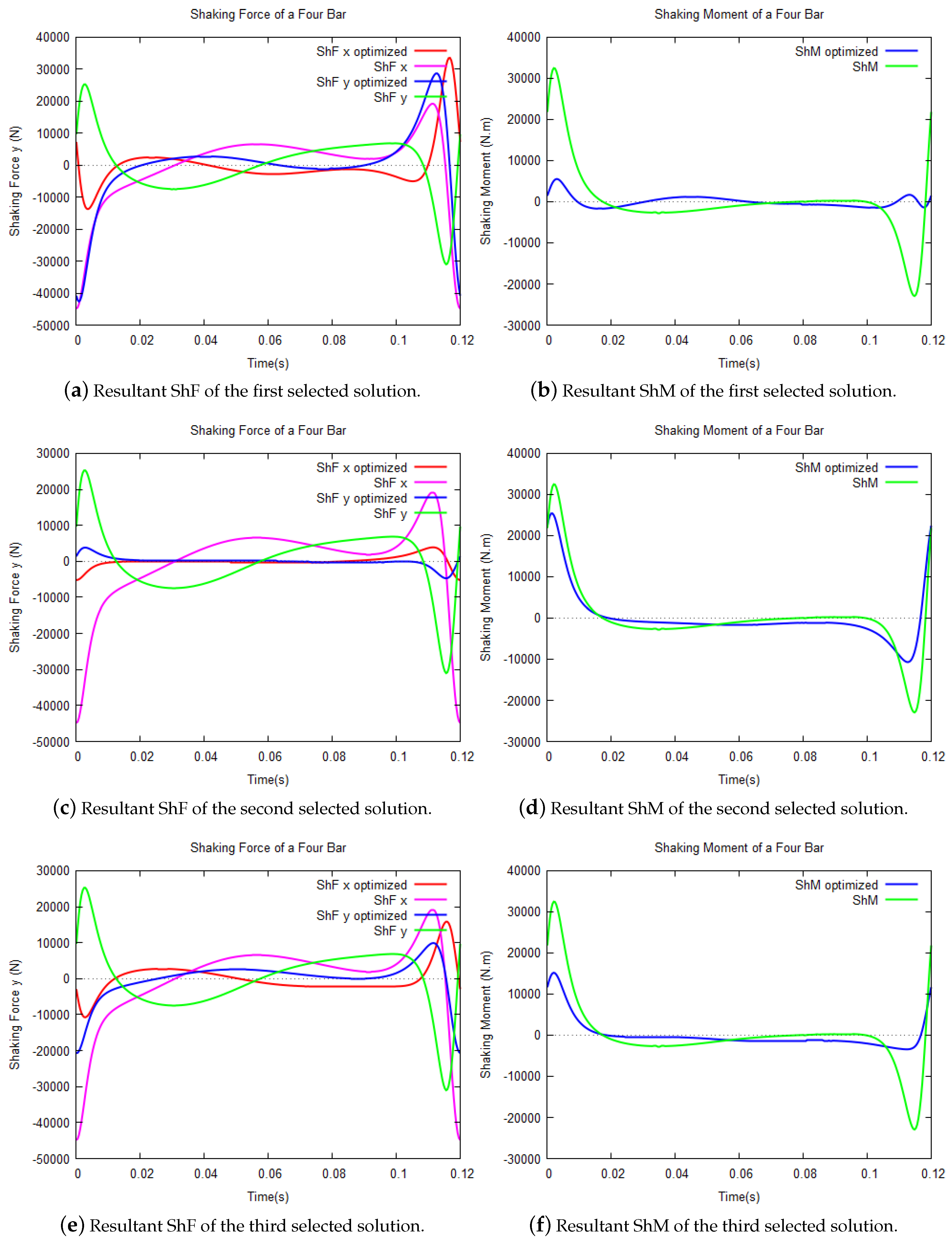
Figure 5a shows the comparison between the ShF (on the x and y axes) of the original mechanism and the ShF after the optimization. In this case, the total ShF was improved only by 8.47%. But with this solution, it is possible to appreciate that the ShM of the four-bar optimized mechanism is 83.99% better than the original one (Figure 5b). It can be observed that upon the sole use of counterweights, it is not possible to eliminate the ShM, but it can be significantly reduced, reducing also the ShF a bit.

The second chosen solution is the one in the Pareto front with the minimum value in ${\beta }_{ShF}$ (${\beta }_{ShM}=0.71311372$, ${\beta }_{ShF}=0.00295769$). It corresponds to the following variables values:

$x_{c1}=-0.15548064\hspace{1em}$	$y_{c1}=-0.007810097\hspace{1em}$	$t_{c1}=0.035743454$
$x_{c2}=-0.046683398\hspace{1em}$	$y_{c2}=-0.068805445\hspace{1em}$	$t_{c2}=0.027404923$
$x_{c3}=-0.132085338\hspace{1em}$	$y_{c3}=0.015127099\hspace{1em}$	$t_{c3}=0.037640418$

In Figure 5c, it is possible to appreciate that the ShF is significantly reduced (99.70%) compared to the original mechanism. It can be considered that the ShF is almost completely eliminated by using counterweights and also that the ShM has a reduction of 28.69% (Figure 5d).

The third chosen solution is the one in the Pareto front where both indexes corresponding to ShF and ShM are optimized almost by 60% (${\beta }_{ShM}=0.42969434$, ${\beta }_{ShF}=0.45176319$). It corresponds to the following variables values:

$x_{c1}=-0.233449901\hspace{1em}$	$y_{c1}=0.047539111\hspace{1em}$	$t_{c1}=0.005$
$x_{c2}=0.0000527\hspace{1em}$	$y_{c2}=0.000296052\hspace{1em}$	$t_{c2}=0.005000159$
$x_{c3}=-0.125584323\hspace{1em}$	$y_{c3}=0.058770112\hspace{1em}$	$t_{c3}=0.04$

By using these counterweights, the ShM is reduced by 57.03% and the ShF by 54.82% (Figure 5e,f).

5.1.4. Partial Derivatives, Volumes and Relation Area-Thickness of Three Counterweights

This subsection presents an analysis to determine if the proposed limits for optimization are the most suitable or if they should be changed (in case there is the possibility of modifying them due to mechanical constraints).

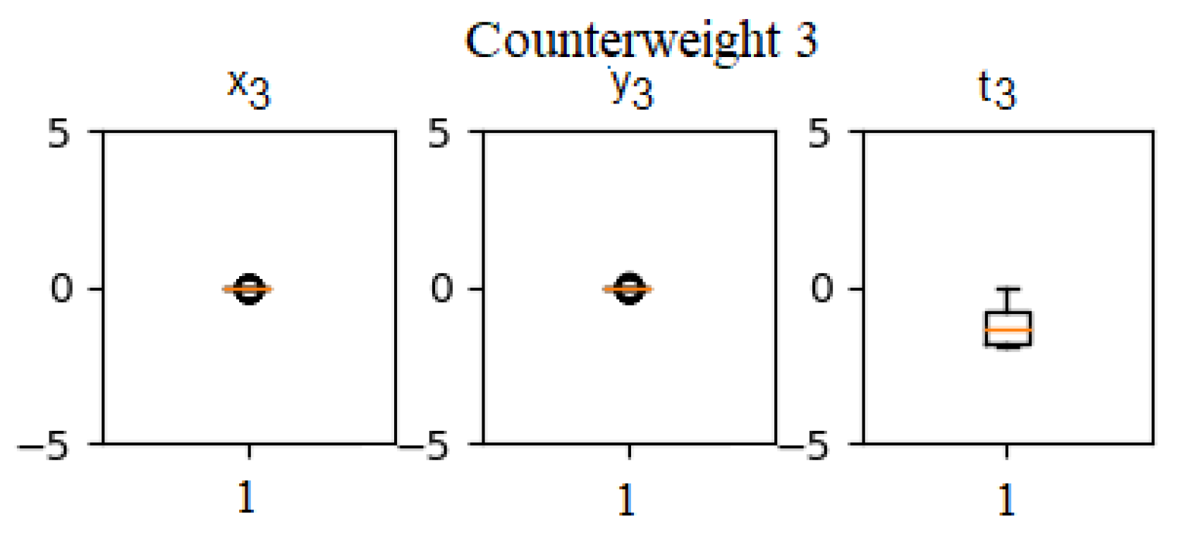
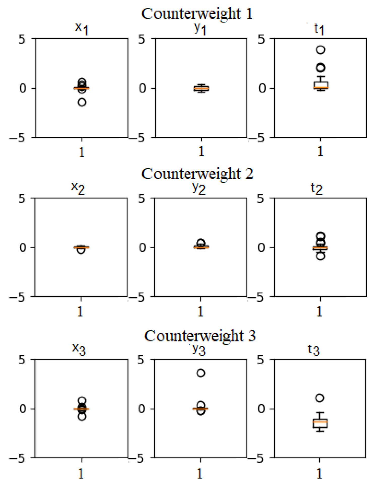
In Figure 6 the box-plots of the partial derivatives with respect to each variable $x_n$, $y_n$ and $t_n$ for each counterweight n ($1\le n\le 3$) are shown.

It is known that an optimal solution is found if all the partial derivatives values are equal to zero. In the box plots of Figure 6 it can be seen that, for the variables $x_n$ and $y_n$ of the counterweights n ($1\le n\le 3$), the partial derivatives are close to zero, this means that it was possible to reach the optimal values within the proposed optimization limits.

However, for the variables $t_1$ and $t_3$, the partial derivatives are not close to zero. In $t_1$, it can be appreciated that the value tends to be greater than zero, hence, it can be deduced that the thickness of Counterweight-1 is trying to be less than the limit 0.005 m. Evidently, this is not possible due to the mechanical limitations that prevent a counterweight thickness from being too close to zero or negative because it is physically impossible. On the other hand, the value of $t_3$ tends to be less than 0, which means that if the limits of the optimization allowed it, Counterweight-3 would have a thickness greater than 0.04 m. This information, obtained from the partial derivatives analysis, can be very useful to decide the limits of the counterweights when there is the possibility to modify them.

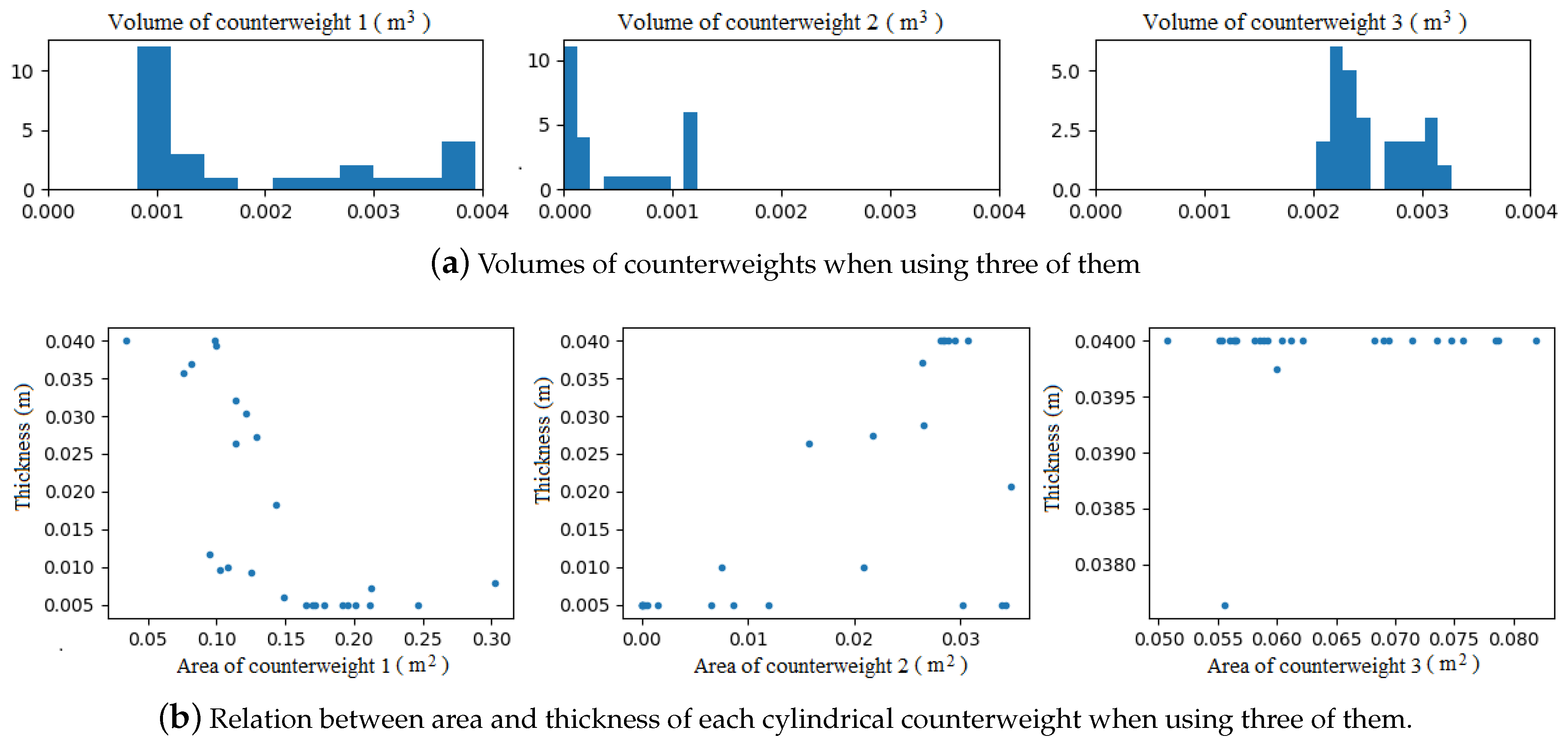
In Figure 7a, the volume value histogram of the counterweights obtained on the different optimization solutions is presented. By analyzing the volume of the counterweights and the relation between their area and thickness (Figure 7b), it can be seen that Counterweight-2 has a very small volume (compared with the other counterweights) and when both area and thickness are very small, Counterweight-2 is almost disappearing from the solution. On the other hand, the relation between the area and the thickness of Counterweight-3 shows how in almost all the cases the thickness is reaching the highest allowed limit; this confirms the information given by the histogram previously analyzed and confirms the conclusion that if mechanical characteristics of the system allows it, it might be advisable to perform the optimization with a slightly larger upper limit for the variable $t_3$.

5.2. Decreasing the Amount of Counterweights Used for Balancing

There could be cases when it is desirable to eliminate one or more counterweights. The reasons can be the resultant volume of the whole mechanism or the cost for implementing the solution.

Pareto Front Comparison to Eliminate One Counterweight

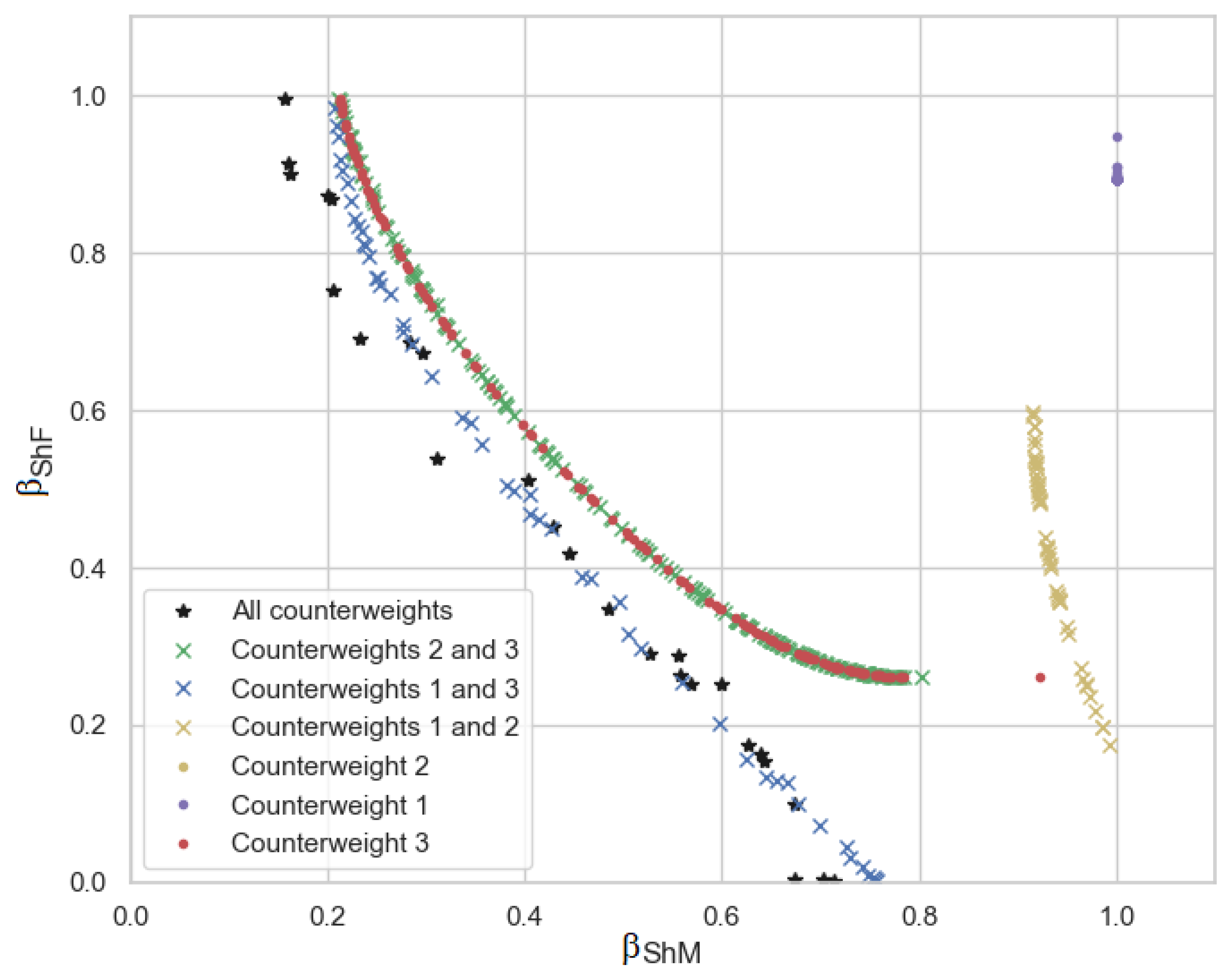
Figure 8 shows the Pareto front of the different optimization results when using all possible combinations (three, two, or only one counterweight). The black stars correspond to the original Pareto front when the three counterweights are used. The blue crosses correspond to the Pareto front when Counterweight-2 has been eliminated and only Counterweights 1 and 3 are being considered. Comparing these results with those obtained when using all the counterweights, it is possible to see that the Pareto fronts are very similar.

The green crosses correspond to the Pareto front when using only Counterweights-2 and 3. The yellow crosses correspond to the Pareto front when Counterweight-3 has been eliminated and Counterweights-1 and 2 are in use.

Using the information provided by the Pareto fronts (Figure 8), it is possible to conclude that, if one decides to eliminate a counterweight to simplify the balancing of the mechanism, it should be Counterweight-2, since using only Counterweights-1 and 3 produces a similar result to that obtained when all three counterweights are used.

Appendix A shows the numerical results when using only two counterweights giving importance to the optimization of the ShF, ShM, and both. A sensitivity analysis is also presented to decide which counterweight should be used if one decides to use only one counterweight. The partial derivatives, volumes and relation area-thickness is also presented giving information about the selected optimization limits, allowing to further improve the results.

Appendix B shows the numerical results when using only one counterweight and presents the sensitivity analysis and the partial derivatives, volumes and relation area-thickness using the methods previously proposed.

Table 2. Comparison between optimization results.

		ShF Optimization	ShM Optimization
Using three counterweights	Optimizing ShF	99.70%	28.69%
	Optimizing ShM	8.47%	83.99%
	Optimizing both ShF and ShM	54.82%	57.03%
Using counterweights 1 and 3	Optimizing ShF	99.67%	24.34%
	Optimizing ShM	1.55%	79.22%
	Optimizing both ShF and ShM	55.05%	57.27%
Using only counterweight 3	Optimizing ShF	78.74%	0.42%
	Optimizing ShM	3.22%	73.61%
	Optimizing both ShF and ShM	51.19%	53.31%

shows the optimization results when using three, two, and one counterweight.

5.3. Expanding Optimization Limits for $t_3$

As aforementioned, using the box-plots of the partial derivatives with respect to each variable, the volume values histogram of the counterweights, and the graphics of the relation between area and thickness, it is possible to obtain valuable information about the chosen limits of the optimization. The decision of modifying these limits depends on the mechanical characteristics of the whole mechanism.

Taking the example when using only one counterweight (Appendix B) the recommendation after the analysis was to choose a higher limit of thickness $t_3$, a new optimization process was executed with the limits:

$$-0.40\mathrm{m}⩽x_{cn},y_{cn}⩽0.40\mathrm{m}$$

(59)

$$0.005\mathrm{m}⩽t_{cn}⩽0.05\mathrm{m}$$

(60)

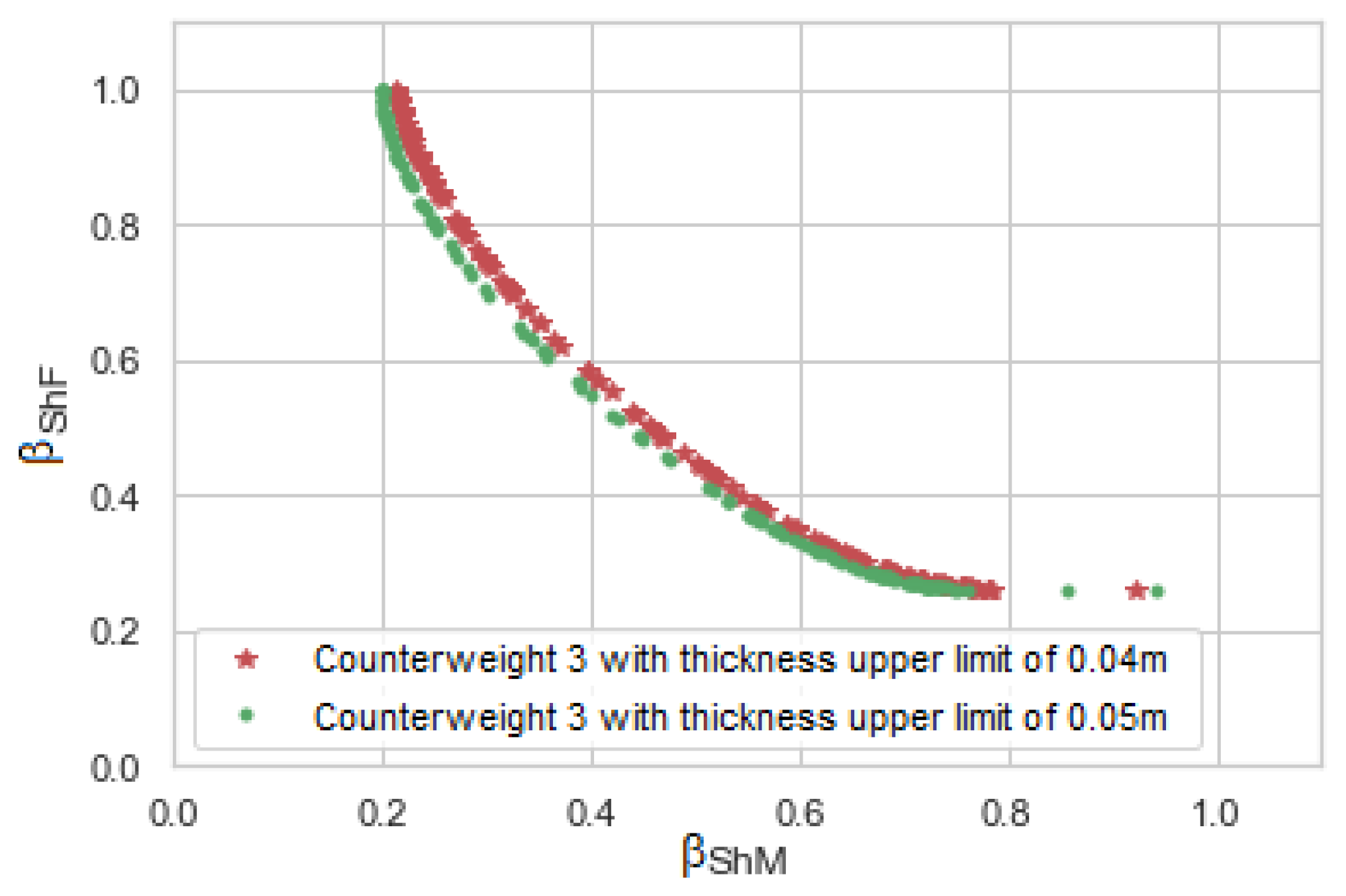
The upper limit of $t_3$ could be changed from 0.04 m to 0.05 m. Using this value and giving more importance to ${\beta }_{ShF}$, the physical characteristics of Counterweight-3 should be:

$x_{c3}=-0.141021300369708\hspace{1em}$

$y_{c3}=-0.00665773774579448\hspace{1em}$

$t_{c3}=0.0207544372440781$

Using this solution, allows the ShF and ShM to be reduced by $73.92\%$ and $14.32\%$, respectively.

On the other hand, when the importance is given to ${\beta }_{ShM}$, the physical characteristics of Counterweight-3 should be:

$x_{c3}=-0.1112378507983744\hspace{1em}$

$y_{c3}=0.091294702876245\hspace{1em}$

$t_{c3}=0.05$

Using this counterweight the ShM and ShF is reduced by $80.17\%$ and $5.30\%$, respectively.

Table 3. Comparison between optimization results when expanding the thickness upper limit of Counterweight-3.

		ShF Optimization	ShM Optimization
Using 0.05 m as $t_3$ upper limit	Optimizing ShF	73.92%	14.32%
	Optimizing ShM	5.30%	80.17%
Using 0.04 m as $t_3$ upper limit	Optimizing ShF	78.74%	0.42%
	Optimizing ShM	3.22%	73.61%

compares the optimization results obtained with the expanded limits and the original limits. It can be seen that expanding Counterweight-3 thickness upper limit, improves the ShM. Figure 9 shows the comparison of Pareto fronts before and after changing the optimization limits. It can be noticed that the thickness of Counterweight-3 has a greater influence on the optimization of the ShM of the mechanism. By increasing this limit, optimization results can be better.

6. Conclusions

By using fully Cartesian coordinates to represent a mechanism, the equations that define the reactions are less complex than those obtained with other methods, hence, the use of this kind of coordinates is suitable for complete balancing, minimization of reactions, and calculation of the ShF and ShM in mechanisms.

The use of fully Cartesian coordinates to represent a four-bar linkage in conjunction with the Simplified Gradient Descent algorithm is a suitable methodology to optimize the balancing of mechanisms. It allows, when using three counterweights and giving more importance to static balancing, to reduce the ShF and ShM by 99.70% and 28.69%, respectively; and when importance is given to the dynamic balancing, to reduce the ShM and the ShF by 83.99% and 8.47%, respectively.

The optimization algorithm was successfully applied to solve the problem. The use of linear combination of functions is a simple yet robust way to handle multi-objectives. The approximation of the derivatives based on Finite Difference allows guiding the algorithm and reducing human hand calculation mistakes.

Comparison between Pareto fronts proves to be an adequate methodology for the sensitivity analysis of each counterweight. This method has proved that even when using only one counterweight, the ShF can be reduced by 78.74% when giving importance to the static balancing or the ShM can be reduced by 73.61% when giving importance to dynamic balancing.

The box-plots of the partial derivatives with respect to each variable, histograms of volumes, and relations between area and thickens allow to analyze the proposed optimization limits in order to decide if they can be changed to obtain even better results.

As future work, it is expected to use these algorithms and analysis to optimize more complex mechanisms in two and three dimensions.

References

- Martini, A.; Troncossi, M.; Rivola, A. Elastodynamic effects of mass-balancing: Experimental investigation of a four-bar linkage. Adv. Mech. Eng. 2013, 2013. [Google Scholar] [CrossRef]
- Zhang, J.; McInnes, C.R. Reconfiguration of a four-bar mechanism using phase space connections. Mech. Syst. Signal Process. 2016, 81, 43–59. [Google Scholar] [CrossRef]
- Arakelian, V.; Dahan, M.; Smith, M. A Historical Review of the Evolution of the Theory on Balancing of Mechanisms. In International Symposium on History of Machines and Mechanisms Proceedings HMM 2000; Springer: Dordrecht, The Netherlands, 2000; pp. 291–300. [Google Scholar] [CrossRef]
- Arakelian, V.H.; Smith, M.R. Shaking Force and Shaking Moment Balancing of Mechanisms: A Historical Review With New Examples. J. Mech. Des. 2005, 127, 334. [Google Scholar] [CrossRef]
- Lowen, G.; Tepper, F.; Berkof, R. Balancing of linkages—An update. Mech. Mach. Theory 1983, 18, 213–220. [Google Scholar] [CrossRef]
- Arakelian, V.; Briot, S. Balancing of Linkages and Robot Manipulators; Mechanisms and Machine Science; Springer International Publishing: Cham, Switzerland, 2015; Volume 27, pp. XVI, 291. [Google Scholar] [CrossRef]
- De Jalón, J.G. Twenty-five years of natural coordinates. Multibody Syst. Dyn. 2007, 18, 15–33. [Google Scholar] [CrossRef]
- García de Jalón, J.; Serna, M.A.; Avilés, R. Computer method for kinematic analysis of lower-pair mechanisms—I velocities and accelerations. Mech. Mach. Theory 1981, 16, 543–556. [Google Scholar] [CrossRef]
- De Jalon, J.G.; Bayo, E. Kinematic and Dynamic Simulation of Multibody Systems: The Real-Time Challenge; Springer: New York, NY, USA, 1994; p. 440. [Google Scholar]
- Chaudhary, K.; Chaudhary, H. Optimal dynamic balancing and shape synthesis of links in planar mechanisms. Mech. Mach. Theory 2015, 93, 127–146. [Google Scholar] [CrossRef]
- Haines, R. Minimum RMS shaking moment or driving torque of a force-balanced 4-bar linkage using feasible counterweights. Mech. Mach. Theory 1981, 16, 185–195. [Google Scholar] [CrossRef]
- Elliott, J.L.; Tesar, D. The Theory of Torque, Shaking Force, and Shaking Moment Balancing of Four Link Mechanisms. J. Eng. Ind. 1977, 99, 715. [Google Scholar] [CrossRef]
- Wiederrich, J.L.; Roth, B. Momentum Balancing of Four-Bar Linkages. J. Eng. Ind. 1976, 98, 1289–1295. [Google Scholar] [CrossRef]
- Tepper, F.R.; Lowen, G.G. Shaking Force Optimization of Four-Bar Linkage With Adjustable Constraints on Ground Bearing Forces. J. Eng. Ind. 1975, 97, 643–651. [Google Scholar] [CrossRef]
- Lowen, G.G.; Berkof, R.S. Determination of Force-Balanced Four-Bar Linkages With Optimum Shaking Moment Characteristics. J. Eng. Ind. 1971, 93, 39–46. [Google Scholar] [CrossRef]
- Berkof, R.S.; Lowen, G.G. Theory of Shaking Moment Optimization of Force-Balanced Four-Bar Linkages. J. Eng. Ind. 1971, 93, 53–60. [Google Scholar] [CrossRef]
- Farmani, M.R.; Jaamialahmadi, A.; Babaie, M. Multiobjective optimization for force and moment balance of a four-bar linkage using evolutionary algorithms. J. Mech. Sci. Technol. 2011, 25, 2971–2977. [Google Scholar] [CrossRef]
- Zamuda, A.; Brest, J.; Boskovic, B.; Zumer, V. Differential evolution for multiobjective optimization with self adaptation. In Proceedings of the 2007 IEEE Congress on Evolutionary Computation, Singapore, 25–28 September 2007; pp. 3617–3624. [Google Scholar] [CrossRef]
- Bulatović, R.; Bošković, M.; Šalinić, S.; Miodragović, G. Multiobjective optimization for dynamic balancing of four-bar mechanism. In Proceedings of the 6th International Congress of Serbian Society of Mechanics, Mountain Tara, Serbia, 19–21 June 2017. [Google Scholar]
- Demeulenaere, B.; Aertbeliën, E.; Verschuure, M.; Swevers, J.; De Schutter, J. Ultimate Limits for Counterweight Balancing of Crank-Rocker Four-Bar Linkages. J. Mech. Des. 2006, 128, 1272. [Google Scholar] [CrossRef][Green Version]
- Nocedal, J.; Wright, S.J. Numerical Optimization; Springer: Berlin/Heidelberg, Germany, 2006; p. 664. [Google Scholar]
- Orvananos-Guerrero, M.T.; Sanchez, C.N.; Davalos-Orozco, O.; Rivera, M.; Velazquez, R.; Acevedo, M. Using Fully Cartesian Coordinates to Calculate the Support Reactions of Multi-Scale Mechanisms. In Proceedings of the 2018 Nanotechnology for Instrumentation and Measurement, NANOfIM 2018, Mexico City, Mexico, 7–8 November 2018; Institute of Electrical and Electronics Engineers Inc.: Piscataway, NJ, USA, 2019. [Google Scholar] [CrossRef]
- Norton, R.L. Design of Machinery: An Introduction to the Synthesis And Analysis of Mechanisms and Machines; McGraw-Hill Higher Education: New York, NY, USA, 2004; p. 858. [Google Scholar]
- Lowen, G.; Tepper, F.; Berkof, R. The quantitative influence of complete force balancing on the forces and moments of certain families of four-bar linkages. Mech. Mach. Theory 1974, 9, 299–323. [Google Scholar] [CrossRef]
- Acevedo, M. Conditions for Dynamic Balancing of Planar Parallel Manipulators Using Natural Coordinates and their Application. In Proceedings of the 14th IFToMM World Congress, Taipei, Taiwan, 25–30 October 2015; pp. 419–427. [Google Scholar] [CrossRef]
- Acevedo, M.; Orvañanos, T.; Velázquez, R. Shaking Moment Balancing of a Four-Bar Mechanism Using Actuation Redundancy. In Mechanisms and Machine Science; Springer: Dordrecht, The Netherlands, 2019; Volume 73, pp. 3319–3327. [Google Scholar] [CrossRef]
- Chong, E.K.; Zak, S.H. An Introduction to Optimization, 2nd ed.; John Wiley & Sons: Hoboken, NJ, USA, 2013; p. 640. [Google Scholar]
- Khademi, G.; Mohammadi, H.; Simon, D. Gradient-Based Multi-Objective Feature Selection for Gait Mode Recognition of Transfemoral Amputees. Sensors 2019, 19, 253. [Google Scholar] [CrossRef]
- Wang, Q.; Yin, J.; Noureldin, A.; Iqbal, U.; Wang, Q.; Yin, J.; Noureldin, A.; Iqbal, U. Research on an Improved Method for Foot-Mounted Inertial/Magnetometer Pedestrian-Positioning Based on the Adaptive Gradient Descent Algorithm. Sensors 2018, 18, 4105. [Google Scholar] [CrossRef]
- Domingo-Perez, F.; Lazaro-Galilea, J.L.; Bravo, I.; Gardel, A.; Rodriguez, D. Optimization of the Coverage and Accuracy of an Indoor Positioning System with a Variable Number of Sensors. Sensors 2016, 16, 934. [Google Scholar] [CrossRef]
- Emmerich, M.T.; Deutz, A.H. A tutorial on multiobjective optimization: Fundamentals and evolutionary methods. Nat. Comput. 2018, 17, 585–609. [Google Scholar] [CrossRef]
- Bergstra, J.; Bengio, Y. Random Search for Hyper-Parameter Optimization. J. Mach. Learn. Res. 2012, 13, 281–305. [Google Scholar]
© 2019 by the authors. Licensee MDPI, Basel, Switzerland. This article is an open access article distributed under the terms and conditions of the Creative Commons Attribution (CC BY) license (http://creativecommons.org/licenses/by/4.0/).