Kinematic Model and Real-Time Path Generator for a Wire-Driven Surgical Robot Arm with Articulated Joint Structure

Abstract

This paper presents a forward kinematic model of a wire-driven surgical robot arm with an articulated joint structure and path generation algorithms with solutions of inverse kinematics. The proposed methods were applied to a wire-driven surgical robot for single-port surgery. This robot has a snake-like robotic arm with double segments to fit the working space in a single port and a joint structure to secure stiffness. The accuracy of the model is highly important because small surgical robot arms are usually controlled by open-loop control. A curvature model is widely used to describe and control a continuum robotic body. However, the model is quite different from a continuum robotic arm with a joint structure and can lead to slack of the driving wires or decreased stiffness of the joints. An accurate forward kinematic model was derived to fit the actual hardware structure via the frame transformation method. An inverse kinematic model from the joint space to the wire-length space was determined from an asymmetric model for the joint structure as opposed to a symmetric curvature model. The path generation algorithm has to generate a command to send to each actuator in open-loop control. Two real-time path generation algorithms that solve for inverse kinematics from the task space to the joint space were designed and compared using simulations and experiments. One of the algorithms is an optimization method with sequential quadratic programming (SQP), and the other uses differential kinematics with a PID (Proportional-Integral-Derivative) control algorithm. The strengths and weaknesses of each algorithm are discussed.

1. Introduction

Minimally invasive surgery has been a continuing medical trend because it can reduce the pain and the recovery time of patients. Robotic surgery has emerged as a solution for minimally invasive surgery. Diverse continuum robot manipulators are being developed for laparoscopic or endoscopic surgery [1]. The most well-known surgical robot system is the da Vinci system (Intuitive Surgical Inc., CA), which has been successfully used in various surgeries in the past decade. Its efficiency has been verified in various ways [2].

The da Vinci Si and Xi have wire-driven robotic arms for multiport surgery. Robot arms access the surgical target through multiple ports [3], but many studies have tried to reduce the number of ports. The da Vinci Si can perform single-port surgery using new curved instruments [4]. Recently, the da Vinci SP was developed specifically for single-port surgery [5]. Another type of wire-driven robot is the SPORT Surgical System (TITAN Medical, Canada) [6], which has triple-segment robot arms with a slit structure and can carry out smooth motion in a single port. Furthermore, flexible surgical robot arms that can be attached to endoscopes were developed to perform endoluminal surgery [7], and an interleaved continuum-rigid manipulator was studied to improve dexterous workspace and accurate actuation [8].

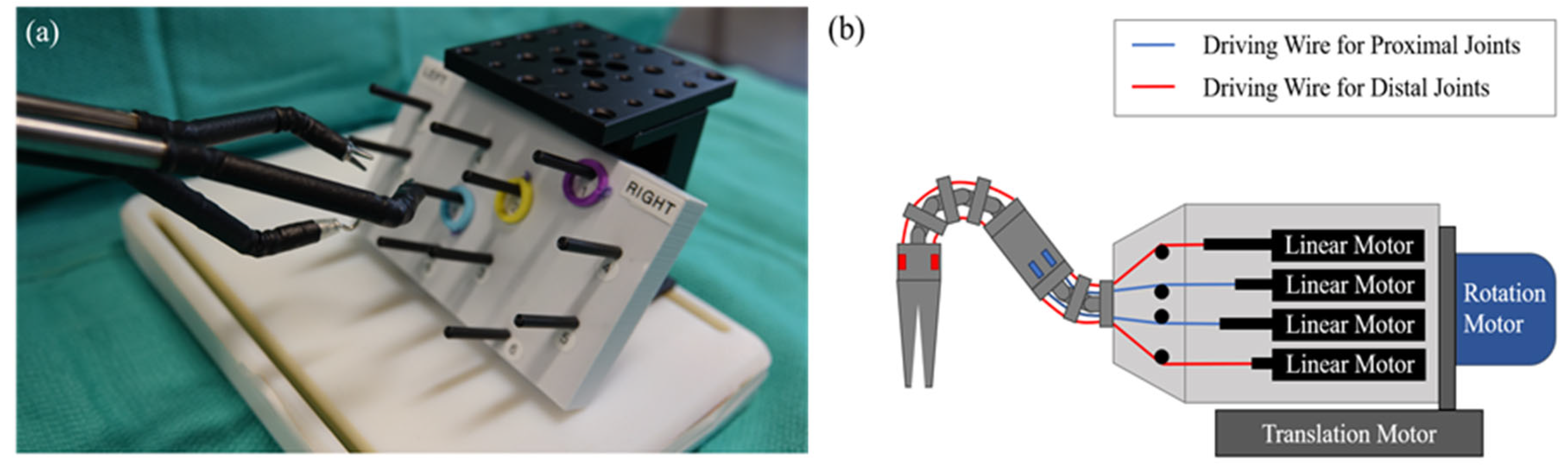
We are developing a wire-driven surgical robot for single-port surgery, as shown in Figure 1a. Two major features of this robot are a joint structure to secure stiffness and double segments to fit the working volume in a single port. Most wire-driven robots are symmetrically controlled with rotating pulleys. In such robots, all wires can be controlled independently for precise movement and other features, as shown in Figure 1b. The proximal joints and distal joints each have two degrees of freedom (DoFs), and the whole body is capable of rotational and translational motion. Consequentially, the end-effector can achieve a six-DoF motion.

There are two well-known structures of a snake-like surgical robot arm: the slit structure and the joint structure [9]. The slit structure is a flexible pipe with slits in various patterns, as shown in Figure 2a. The SPORT System is a representative example. The slit structure can make a smoothly curved configuration, and the model is simplified to the curvature model. However, this structure does not have enough stiffness to perform some general surgical operations, including sutures.

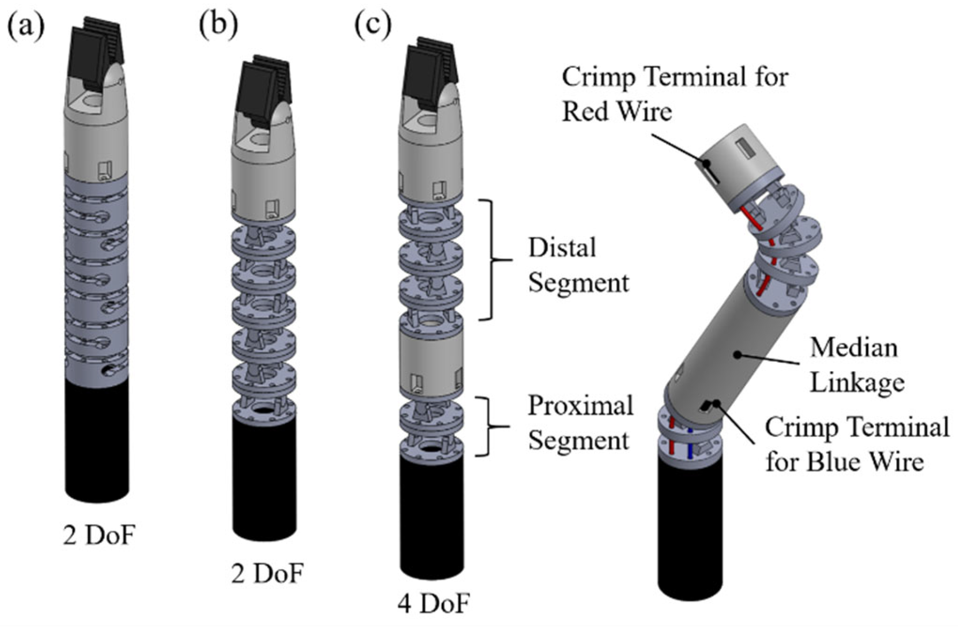
An articulated robot arm with a joint structure consists of orthogonally stacked joints, as shown in Figure 2b. One example is the da Vinci Si. A joint structure cannot be curved in a perfect curvature configuration, but it has stronger stiffness than a slit structure. The set of stacked joints that share the connected wires is called a segment. One segment with orthogonally stacked joints can bend with a two-DoF motion. In single-port surgery, dual robotic arms have to be able to maintain a triangular configuration like a crab’s claw, and an articulated arm with multiple segments is essential to establish the working space, as shown in Figure 2c.

The motion of the distal segments is affected by the motion of the proximal segments because the wires that control the distal segment pass through all stacked joints (see Figure 2c). The blue wire is connected to the median linkage with a wire crimp terminal and controls only the proximal segment. The red wire controls the distal segment and passes through all joints. This phenomenon is called the coupling problem, which must be solved to control robot arms with multiple segments.

The accuracy of the robot model heavily influences the robot’s performance. The robot arm has a tiny structure with a diameter of less than 6 mm. The robot arm operates inside the body, and it is hard to attach encoders or sensors to the arm to measure joint angles or trace the end-effector’s position and orientation. This type of robot is usually controlled by open-loop control based on a mathematical model, unlike general industrial robot arms. The wire driving length has to be calculated from the robot model and a path generation algorithm according to an arbitrary input from the master device in real-time without any feedback from the joint configuration. Therefore, a comparison study about modeling approaches for tendon-actuated continuum robots was carried out [10].

Most snake-like robot arms have been analyzed with a constant-curvature model for convenience [11]. Recently, a variable-curvature model was derived to improve the accuracy of the curvature model [12]. The curvature model works well for a continuum body such as the slit structure, but it does not fit well with a joint structure. The driving wire length is calculated with modeling error, and wire slack behavior may occur between the joints, where the joints are not able to bend to the desired angle or maintain stiffness. In this paper, a more accurate kinematic model was derived to fit an articulated robot arm with a joint structure, and effective path generation algorithms are proposed to solve the inverse kinematics.

One challenging problem is how to solve inverse kinematics from the task space to the wire-length space and generate an actuation path in real-time. A kinematic model of a wire-driven robot arm usually consists of three spaces called the task space, joint space, and wire-length space, as shown in Figure 3. The task space includes the position and orientation of the end-effector, which are given from the master device with the surgeon in real-time. The joint space deals with the joint configuration, which includes the joint angles, translation, and rotation of the robot arm. The wire-length space includes the wire-driving length from the motors.

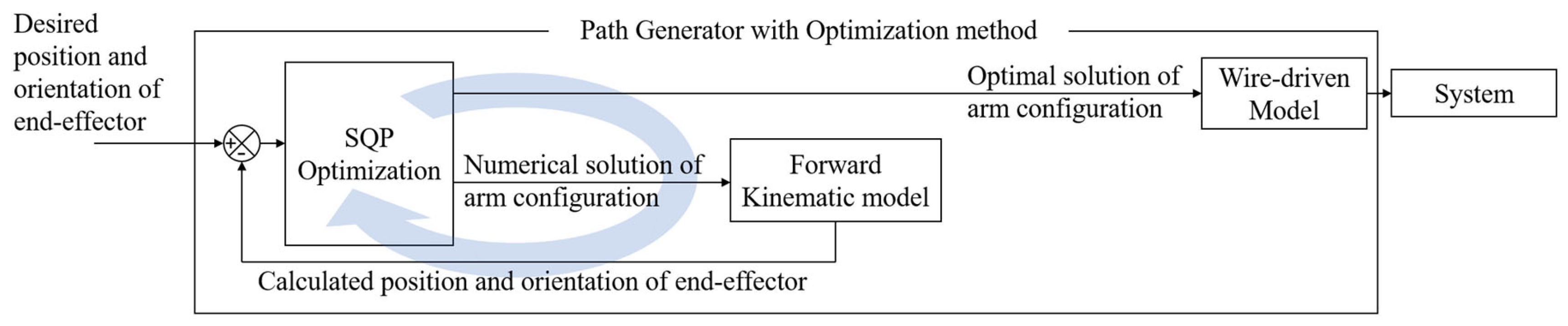
The general approach with the curvature model is to solve the inverse kinematics from the task space to the wire-length space at once. When the coupling problem is solved in multiple segments, however, this approach is restricted by geometrical assumptions [13,14]. In addition, an accurate kinematic model requires more complicated calculations. The numerical method is an effective way to solve inverse kinematics due to the complexity of the forward kinematic model with a joint structure. The sequential quadratic programming (SQP) method is one of the most successful general methods to solve the nonlinearly constrained minimization problem [15]. A combination of SQP and the iterative Newton–Raphson algorithm was used to solve the inverse kinematics of a humanoid robot with redundancy [16]. Recently, an open-source library (TRAC-IK) was developed and distributed for solving inverse kinematics with SQP [17]. As an alternative to the optimization path generator, a path generator was designed using a PID feedback control algorithm. In this method, solving for inverse kinematics is considered to be a feedback control problem, and the analytical solution is derived by inverting the differential kinematics. A short calculation time can be guaranteed because there is no iteration. The stability of the closed-loop inverse kinematics algorithm for redundant robots was verified in the discrete time domain [18]. The closed-loop inverse kinematics algorithm showed advantages in singular value filtering and task priority strategy in comparative experiments of a whole-arm manipulator (WAM) robot [19].

In this study, the solution for inverse kinematics was divided into two steps: one from the task space to the joint space and one from the joint space to the wire-length space. First, an accurate forward kinematic model from the joint space to the task space was derived while considering the joint structure. Then, the joint space solution could be obtained through inverse kinematics. The inverse kinematic model from the joint space to the wire-length space was derived using a modified curvature model. Finally, the two inverse kinematics were connected by substituting the calculated values, which could effectively generate an accurate actuation path corresponding to each wire-driving length in real-time. In this project, tungsten wire was considered to be a rigid structure, and the friction and elongation of the wire were negligible. The robotic arm could be operated only by position control.

This paper proposes two algorithms to solve the inverse kinematics from the forward kinematic model. One of them is a numerical method with sequential quadratic programming (SQP), and the other uses differential kinematics with a control algorithm. In the numerical method, the constraint logic for the mechanical limits of the robot arm works well in real-time, even when a human operator mistakenly manipulates the master device to an excessive value. Compared to another method, the numerical method can easily respond to changes in robot structure, since only the forward kinematic model needs to be replaced without Jacobian or gain tuning. However, calculation speeds due to iteration should always be considered and designed. The differential kinematic method is much faster and much more accurate than the numerical method. However, it cannot restrict the actuation value to the mechanical limits.

The remainder of this paper is organized as follows. Section 2 presents a derivation of the forward kinematic model of the joint structure using frame transformation and compares the results to the curvature model. Section 3 describes the inverse kinematic model from the joint space to the wire-length space with the modified curvature model. The advantages of this model in preventing slack and solving the coupling problem are discussed. Section 4 introduces the two path generation algorithms. The strengths and weaknesses of each algorithm are discussed with simulation results. Section 5 presents experimental results with a surgical robot prototype to verify the feasibility of the path generators. The last section gives a conclusion and discusses future work.

2. Forward Kinematic Model from Joint Space to Task Space

The forward kinematic model was derived using a classical approach with rigid body transformation. Moving frames were attached to each joint, and the relative position and orientation between frames can be described with a homogeneous transformation matrix. The arm has multiple one-DoF revolute joints that are stacked. The axes of the stacked joints are arranged orthogonally to increase the DoFs and secure the wire path [20]. The forward kinematic model can be obtained from the sequential product of the transformation matrices.

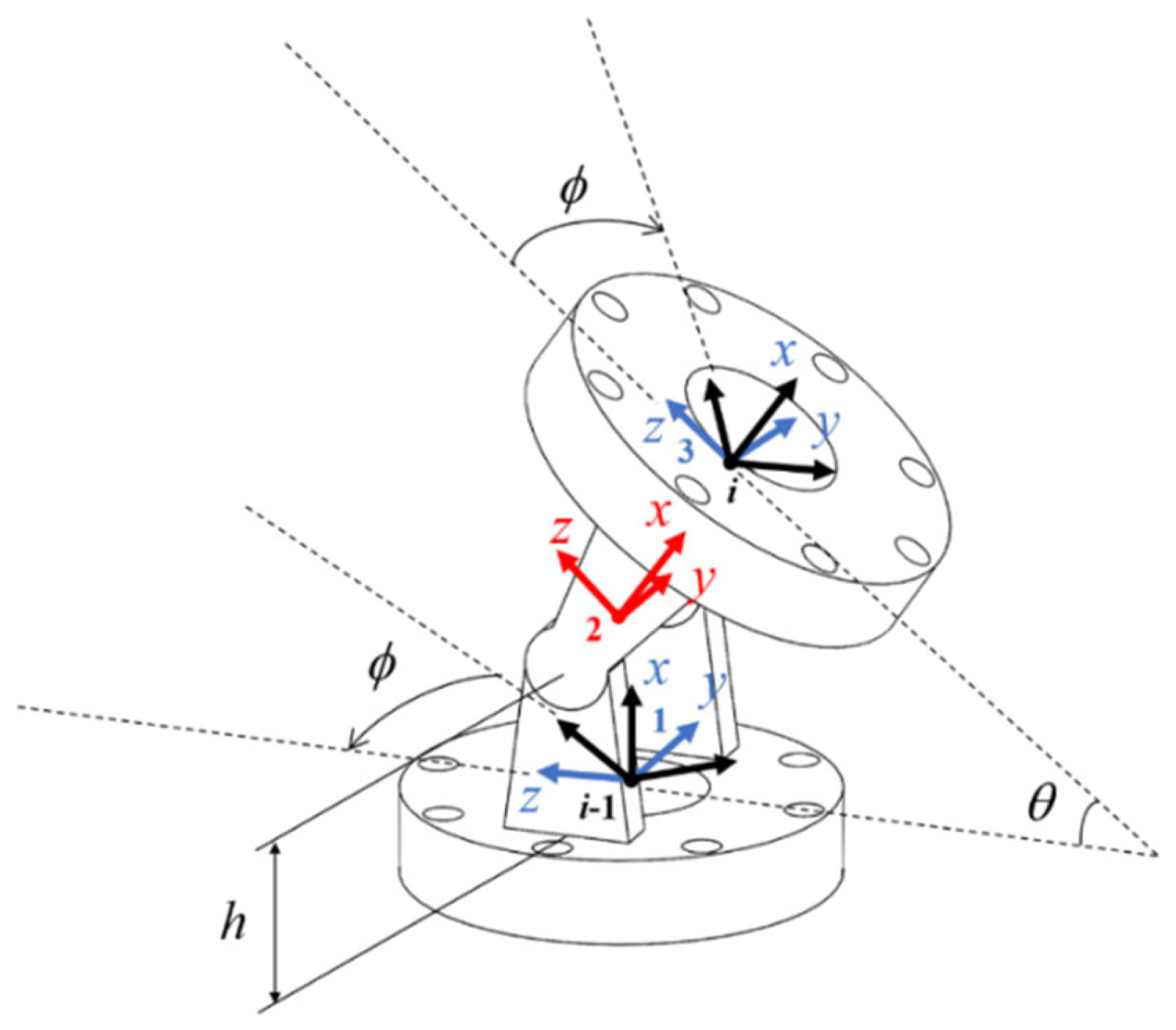
Figure 4 shows a diagram of a single-joint section. The relationship between the i − 1th frame and the ith frame is described by Equation (1) for frames from 1 to 3, where ϕ is the assigned angle of the joint axis, whose parameter is initially determined; θ is the bending angle of the joint, which changes with the joint configuration; and h is the height of the joint axis from the base plane. To produce the transformation matrix of the next joint independently, the assigned angle ϕ has to return to its initial value:

$$\begin{array}{l}{T}^{i-1,i}\left(\varphi ,\theta \right)=T^{i-1,1}\left(\varphi \right)T^{1,2}\left(\theta \right)T^{2,3,i}\left(-\varphi \right)\\ =\left[\begin{array}{cccc}1& 0& 0& 0\\ 0& \cos \varphi & -\sin \varphi & 0\\ 0& \sin \varphi & \cos \varphi & 0\\ 0& 0& 0& 1\end{array}\right]\left[\begin{array}{cccc}\cos \theta & 0& \sin \theta & h\\ 0& 1& 0& 0\\ -\sin \theta & 0& \cos \theta & 0\\ 0& 0& 0& 1\end{array}\right]\left[\begin{array}{cccc}1& 0& 0& h\\ 0& \cos \left(-\varphi \right)& -\sin \left(-\varphi \right)& 0\\ 0& \sin \left(-\varphi \right)& \cos \left(-\varphi \right)& 0\\ 0& 0& 0& 1\end{array}\right]\\ =\left[\begin{array}{cccc}\cos \theta & -\sin \varphi \sin \theta & \cos \varphi \sin \theta & h\left(\cos \theta +1\right)\\ \sin \varphi \sin \theta & {\cos }^2\varphi +\cos \theta {\sin }^2\varphi & -\frac{\sin 2\varphi \left(\cos \theta -1\right)}{2}& h\sin \varphi \sin \theta \\ -\cos \varphi \sin \theta & -\frac{\sin 2\varphi \left(\cos \theta -1\right)}{2}& {\cos }^2\varphi \cos \theta -{\cos }^2\varphi +1& -h\cos \varphi \sin \theta \\ 0& 0& 0& 1\end{array}\right]\end{array}.$$

(1)

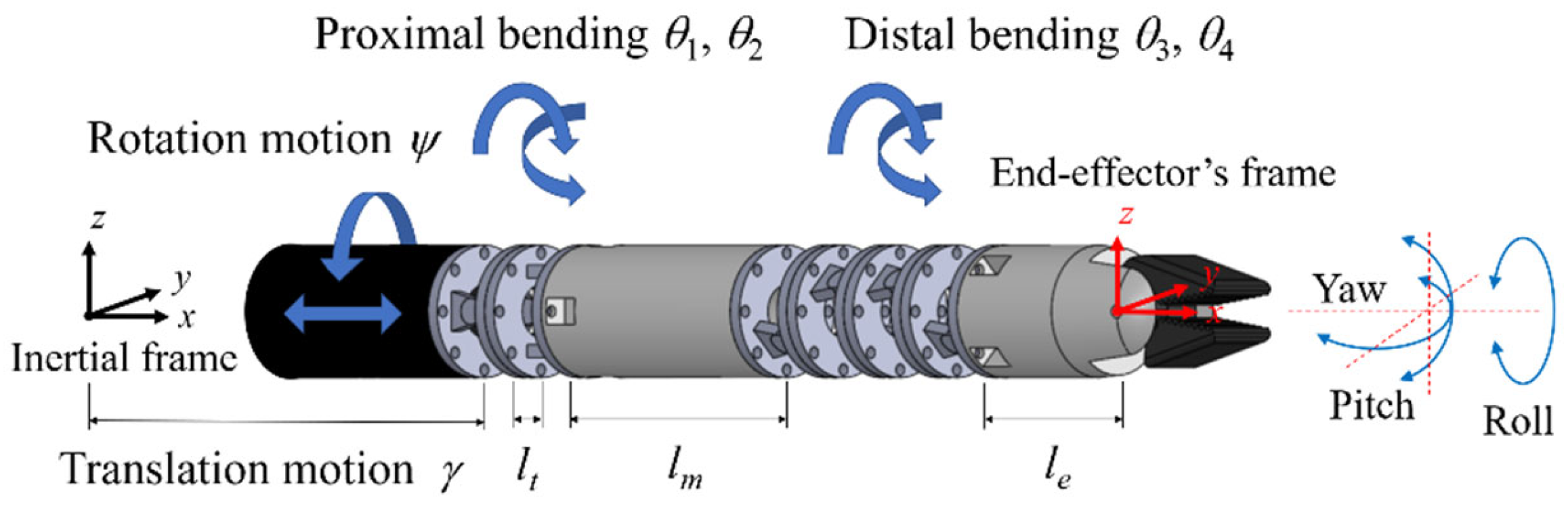
An example is shown in Figure 5. The arm can achieve a six-DoF motion with double segments. The translation motion of the base is γ, and the rolling motion is ψ. The proximal segment has two joints and can simultaneously bend with θ₁ and θ₂ in orthogonal directions. The distal segment has four joints and can bend with θ₃ and θ₄ in orthogonal directions. Each set of two distal joints is coupled. It is assumed that the coupled joints equally share a bending angle.

The thickness between joint bases is l_t, and the lengths of the medial linkage and end-effector are l_m and l_e, respectively. The transformation matrices for the translation motion and rolling motion are Equation (2) and Equation (3), respectively. The matrix G in Equation (4) just moves the frames by the length of the components. The transformation matrix from the inertial frame to the end-effector’s frame can be obtained from the product of the matrices, as shown in Equation (5). In this work, the product of the exponential was used to derive the forward kinematics, and the configuration parameters are arranged in

Table 1. Configuration parameters of articulated joints robotic arm with double segments.

Configuration	Symbol	Value
Height of joint axis	h	1 mm
Thickness between joint bases	lt	1 mm
Length of medial linkage	lm	30 mm
Length of end-effector	le	22 mm

. As a result, the position and orientation of the end-effector can be calculated, as shown in Equation (6), where the subscripts of the matrix represent the number of rows and columns. The orientation is expressed as z–y–x Euler angles for the roll, pitch, and yaw. This is the exact forward kinematic model of the articulated robotic arm with a joint structure.

Equations (2)–(6) are

$$\mathrm{Tr}(\gamma )=\left[\begin{array}{cccc}1& 0& 0& \gamma \\ 0& 1& 0& 0\\ 0& 0& 1& 0\\ 0& 0& 0& 1\end{array}\right],$$

(2)

$$\mathrm{Ro}(\psi )=\left[\begin{array}{cccc}1& 0& 0& 0\\ 0& \cos \psi & -\sin \psi & 0\\ 0& \sin \psi & \cos \psi & 0\\ 0& 0& 0& 1\end{array}\right],$$

(3)

$$G(l)=\left[\begin{array}{cccc}1& 0& 0& l\\ 0& 1& 0& 0\\ 0& 0& 1& 0\\ 0& 0& 0& 1\end{array}\right],$$

(4)

$$\begin{array}{l}T\left(\gamma ,\psi ,{\theta }_1,{\theta }_2,{\theta }_3,{\theta }_4\right)=\mathrm{Tr}\left(\gamma \right)\mathrm{Ro}\left(\psi \right)T^{0,1}\left(0,{\theta }_1\right)G\left(l_t\right)T^{1,2}\left(\frac{\pi }{2},{\theta }_2\right)G\left(l_m\right)T^{2,3}\left(\frac{\pi }{4},\frac{{\theta }_3}{2}\right)G\left(l_t\right)T^{3,4}\left(\frac{3\pi }{4},\frac{{\theta }_4}{2}\right)G\left(l_t\right)\\ T^{4,5}\left(\frac{3\pi }{4},\frac{{\theta }_4}{2}\right)G\left(l_t\right)T^{5,6}\left(\frac{\pi }{4},\frac{{\theta }_3}{2}\right)G\left(l_e\right)\end{array},$$

(5)

$$\begin{array}{l}x=T_{1,4},y=T_{2,4},z=T_{3,4},\\ roll=\arctan \left(\frac{T_{3,2}}{T_{3,3}}\right),pitch=\arctan \left(\frac{-T_{3,1}}{\sqrt{T_{3,2}^2+T_{3,3}^2}}\right),yaw=\arctan \left(\frac{T_{2,1}}{T_{1,1}}\right)\end{array}.$$

(6)

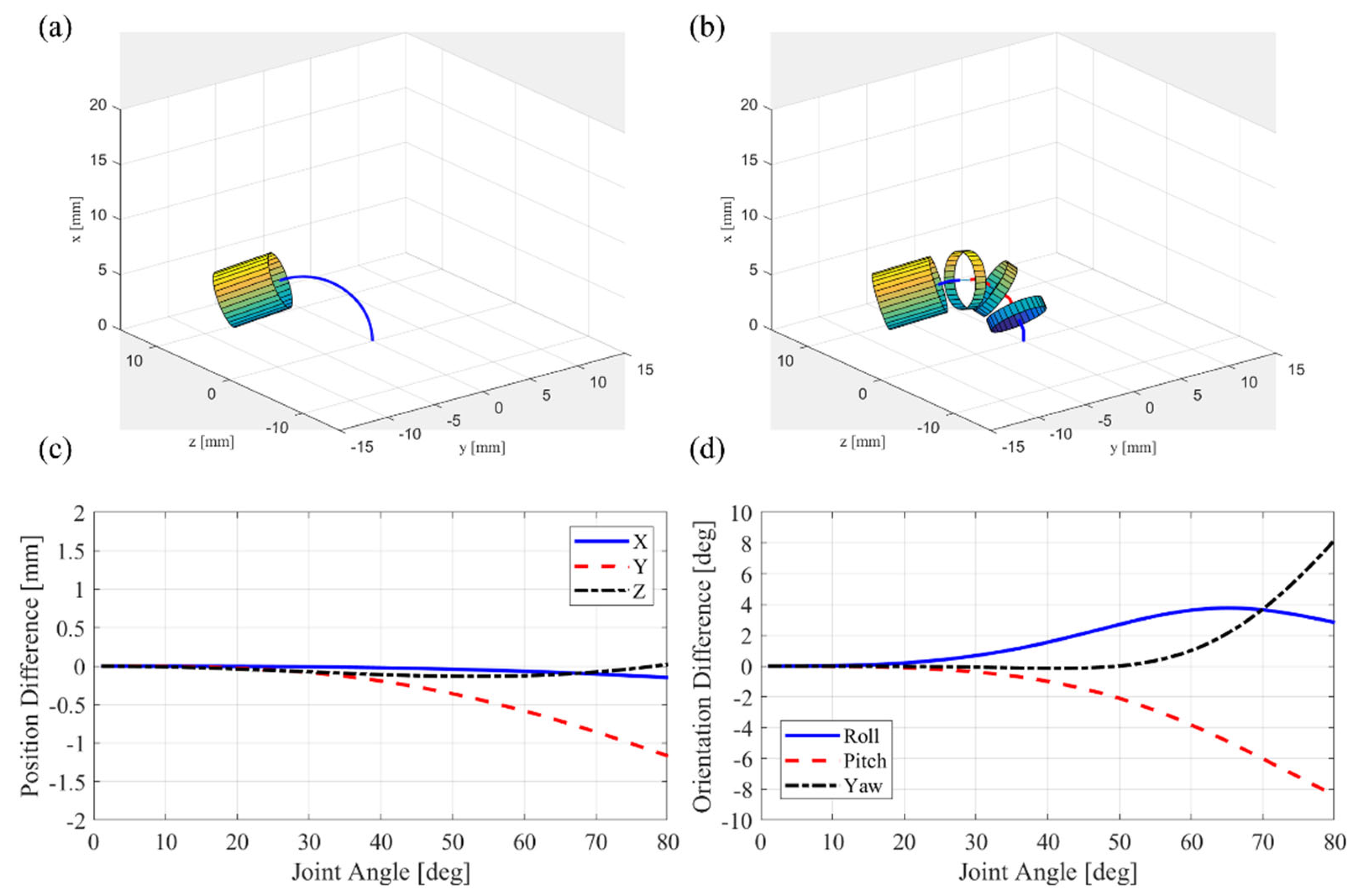
In another example, the forward kinematics of a single-segment robotic arm with four joints is compared between the curvature model and the joint model, as shown in Figure 6a,b. Both orthogonal joints simultaneously bend at equal angles. The position difference between the two models is within about 1 mm, as shown in Figure 6c. The maximum orientation difference is about 8° according to the bending angle, as shown in Figure 6d. When surgeons control the robotic arm using master devices in real-time, they are more sensitive to the orientation error than the position error because it is more visible [21]. An accurate kinematic model helps to make operators more comfortable.

3. Inverse Kinematic Model from Joint Space to Wire-Length Space

The inverse kinematics of a wire-driven robotic arm represent the physical relationship between the task space and the wire-length space. Inverse kinematics are divided into two steps: one from the task space to the joint space and one from the joint space to the wire-length space. First, the inverse kinematic model from the joint space to the wire-length space is derived from a geometric approach.

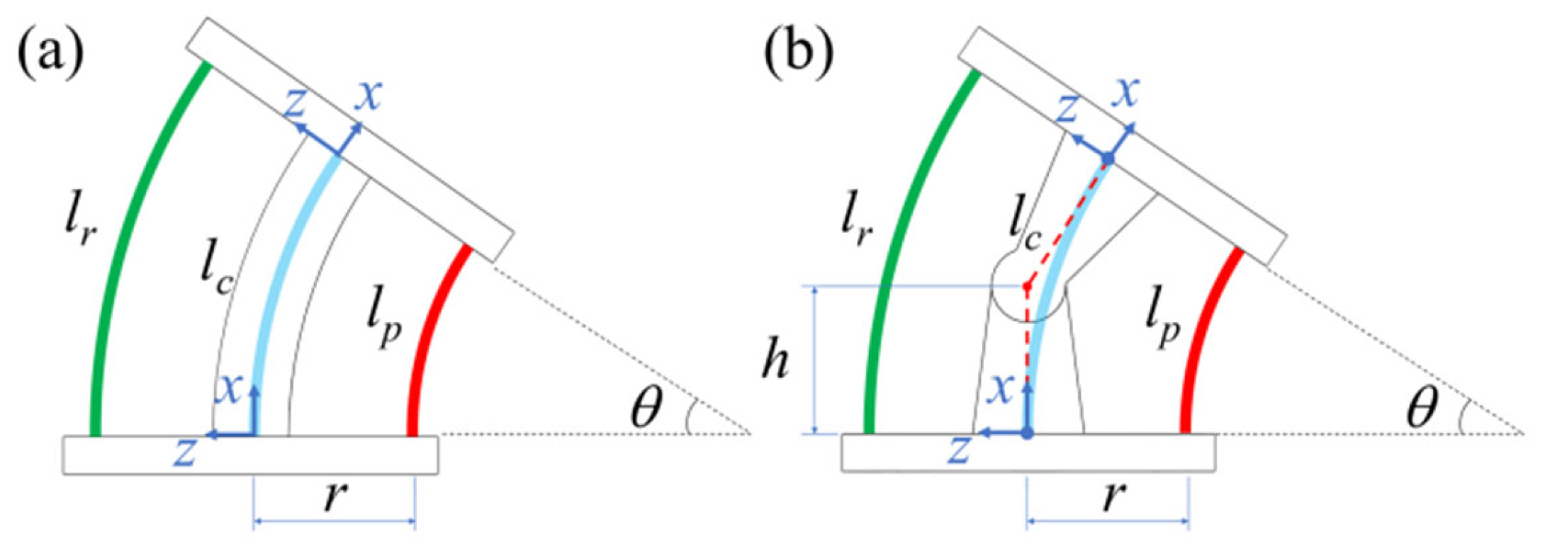
The conventional curvature model starts with an assumption that the arc length at the center is always conserved. However, in the joint structure, the virtual arc length at the center varies with the bending angle. Figure 7 shows a comparison between the curvature model and the joint model. The wire length at the center is l_c, and the outer and inner wire lengths of the bending joint are l_r and l_p, respectively. The distance between the joint axis and the wire is r, and the length of all wires is the same as the linkage height 2h before the joint bends. Each wire length is calculated based on the conventional curvature model shown in Equation (7). The wire length during pulling and that during releasing are symmetric. In this study, h is 1 mm, and r is 2.45 mm.

In the joint structure, the wire length model has to be modified, as shown in Equation (8). The wire lengths during pulling and releasing are not symmetric with respect to the initial wire length in this case. If the wires are driven in accordance with the curvature model, the wires are pulled less and released more compared to the modified model, as shown in Figure 8. Then, slack occurs in the driving wires, and the joint cannot bend to the desired angle or secure stiffness. The modified model with asymmetric lengths for the joint structure guarantees more accurate motion without slack.

The wire length at the center becomes shorter according to the bending angle. In the general case, wires to control the jaws of the end-effector are located at the center of the robotic arm. The jaws of the end-effector are used to not fully close or open in an arm configuration with a large bending angle. This model shows that the driving wire length at the center to actuate the end-effector needs compensation for the bending angle of the joints:

$$\begin{array}{l}{l}_r=2h+r\theta \\ l_p=2h-r\theta \\ l_c=2h\end{array},$$

(7)

$$\begin{array}{l}{l}_r=\left(\frac{h}{\tan \left(\theta /2\right)}+r\right)\theta \\ l_p=\left(\frac{h}{\tan \left(\theta /2\right)}-r\right)\theta \\ l_c=\frac{h\theta }{\tan \left(\theta /2\right)}\end{array}.$$

(8)

Another advantage of this model is that the compensation length for the coupling problem is solved at the same time. In the stacked joint structure, the wires affect all joints that they pass through. When the wire length to actuate a joint is calculated, the bending angles of all joints that the wire has previously passed through have to be considered. Since this wire length model is a function of only the joint angles, all wire lengths are naturally decided according to the joint configuration.

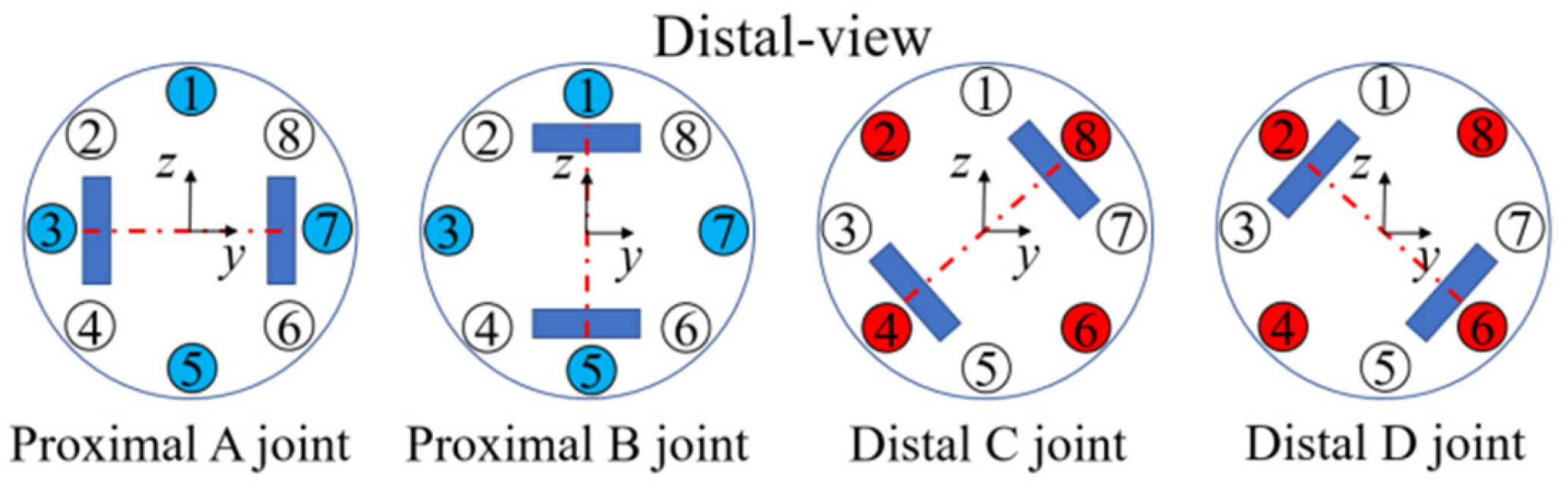
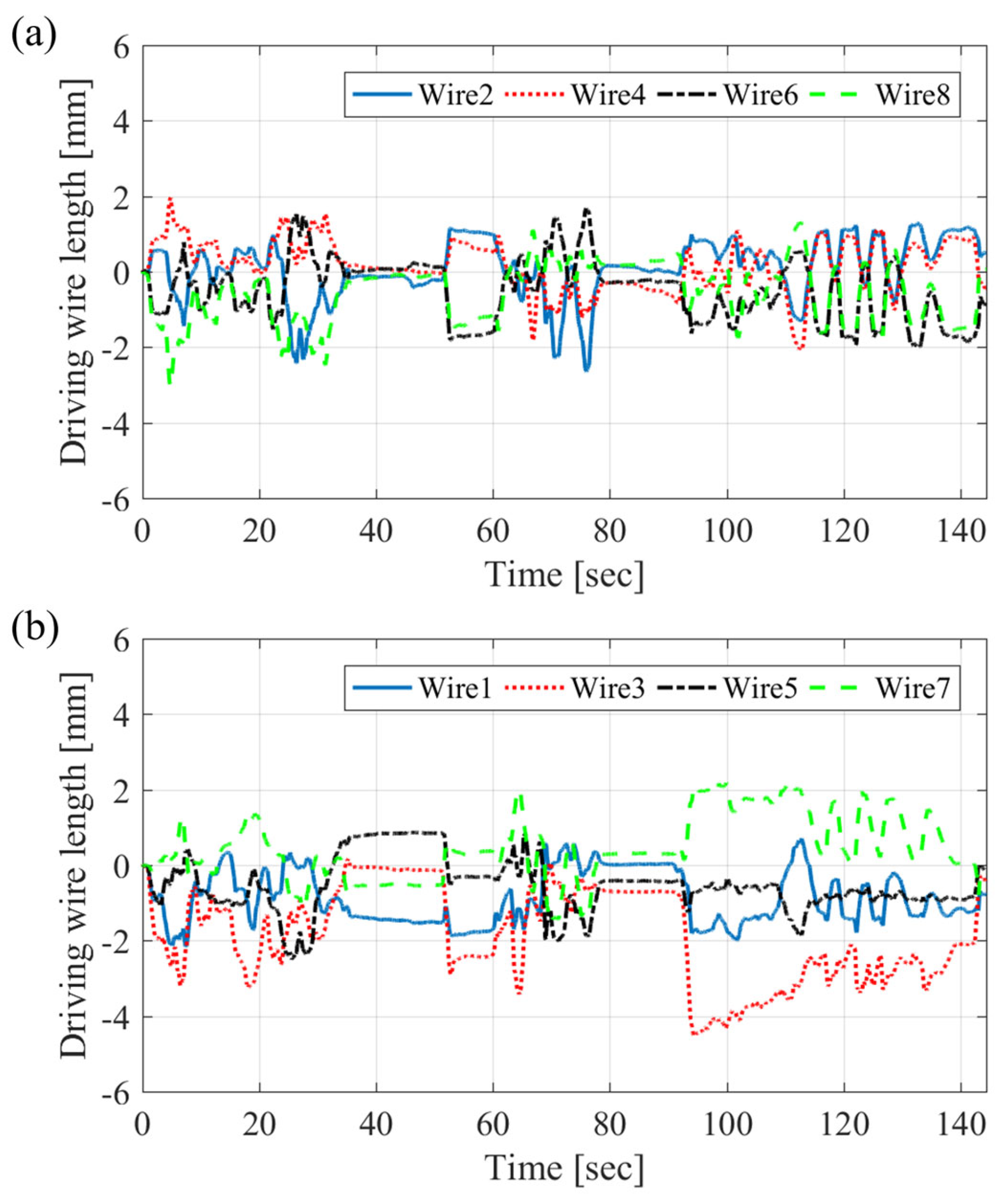
Figure 9 shows views of the distal section from the example in Figure 5. In this case, the arrangement of joints is A–B (proximal)/C–D–D–C (distal). The distal joints are assembled pairs. The two pairs of blue boxes indicate joints, and the red dashed–dotted line across the two blue boxes represents the joint axis. Wires 1, 3, 5, and 7 are connected to proximal joints. Wires 2, 4, 6, and 8 are connected to distal joints through the proximal joints. The driving length of wire 1 is derived as shown in Equation (9):

$$w_1=\left\{2h-\left(\frac{h}{\tan \left|{\theta }_1/2\right|}+\mathrm{sgn}\left({\theta }_1\right)r\right)\left|{\theta }_1\right|\right\}+\left\{2h-\frac{h}{\tan \left|{\theta }_2/2\right|}\left|{\theta }_2\right|\right\},$$

(9)

where sgn() is the sign function.

Wire 1 can control only the proximal joint angle and does not affect the distal joint angle at all. Wire 4 is different from wire 1, and its driving length consists of two parts: the compensation length for proximal joints and the driving length for distal joints, as shown in Equation (10). The compensation length is geometrically determined from the angles of the proximal joints. If the wire length does not properly compensate for the proximal joint angle, the distal joints may bend to an unexpected configuration.

$$\begin{array}{l}{w}_4=compensationlength+drivinglength\\ =\left[\begin{array}{l}\left\{2h-\left(\frac{h}{\tan \left|{\theta }_1/2\right|}-\mathrm{sgn}\left({\theta }_1\right)r\sin \left(\pi /4\right)\right)\left|{\theta }_1\right|\right\}\\ +\left\{2h-\left(\frac{h}{\tan \left|{\theta }_2/2\right|}+\mathrm{sgn}\left({\theta }_2\right)r\sin \left(\pi /4\right)\right)\left|{\theta }_2\right|\right\}\end{array}\right]+\left[\left\{4h-\left(\frac{h}{\tan \left|{\theta }_3/4\right|}\right)\left|{\theta }_3\right|\right\}+\left\{4h-\left(\frac{h}{\tan \left|{\theta }_4/4\right|}+\mathrm{sgn}\left({\theta }_4\right)r\right)\left|{\theta }_4\right|\right\}\right].\end{array}$$

(10)

4. Path Generator Solving for Inverse Kinematics

An accurate forward kinematic model can describe the actual robotic arm motion exactly, but the resulting equations are complicated. It is impossible to solve explicit inverse kinematics, so many studies have attempted to simplify the kinematic model with methods such as the curvature-based model. Another approach is a numerically iterative method to obtain the solution of inverse kinematics. The optimization method used to be applied to solve the inverse kinematics of a soft robot [22] and a continuum robot [23]. Redundant snakelike robot teleoperation was controlled using the pseudoinverse of Jacobian and linear programming [24]. In this study, the inverse kinematics from the task space to the joint space were solved in two different ways: a numerical method and an approach using differential kinematics with a control algorithm. The inverse kinematic solution from the task space to the joint space is used in the inverse kinematic model from the joint space to the wire-length space, which means the path of each linear actuator for driving the wires can be generated in real-time. The path generator means a transformation algorithm for position control from the task space trajectory into the actuation space trajectory was used in this project.

4.1. Optimization Method with Sequential Quadratic Programming

This paper employs SQP to solve the complex inverse kinematic model with joint limits. This algorithm numerically searches for the optimal solution of the robot arm configuration corresponding to the desired position and orientation of the end-effector. The objective function is the minimization of the norm of the six-DoF errors between the desired position and orientation and the calculated values from the forward kinematic model. The constraint is the mechanical actuation limits. The objective function and the constraints can be described as Equation (11). The position and orientation errors are nondimensionalized, with division by 1 mm and 1°, respectively, used to calculate the six-DoF error norm. Each step finds the converged solution with iteration, and the initial value of each step is obtained from the solution in the previous step. In each step, wire-driven actuation values are calculated from the optimal solution of inverse kinematics of arm configuration through the wire-driven model. An open-loop control process with the optimization path generator is shown as a block diagram in Figure 10. The computation time for each step due to iteration is a critical issue in this approach. The computing power of the controller should be considered to implement this method. Equation (11) is

$$\begin{array}{l}\underset{{\theta }_1,{\theta }_2,{\theta }_3,{\theta }_4,\gamma ,\psi }{{\displaystyle \min .}}\sqrt{e_x^2+e_y^2+e_z^2+e_{roll}^2+e_{pitch}^2+e_{yaw}^2}\\ subjectto-45°<{\theta }_1<45°\\ -45°<{\theta }_2<45°\\ -90°<{\theta }_3<90°\\ -90°<{\theta }_4<90°\\ -50mm<\gamma <50mm\\ -180°<\psi <180°\end{array}.$$

(11)

The proposed path generator with the optimization algorithm was tested with the motion of the robot arm. Suturing tasks are the most important missions of this robot. The desired position and orientation were generated and recorded by surgeons to simulate the motions of suturing using an Omega 6 haptic master device (Force Dimension, Switzerland). This study sampled one of the most knotty paths to implement from several trajectories, as shown in Figure 11. The path generator calculates the joint angles, translation stroke, and rotation angle by solving for the inverse kinematics, as shown in Figure 12. The computation loop time is fixed as 10 ms. These actuation values are used in the forward kinematics, and the error of the path generator can be derived as shown in Figure 13. The error increased dramatically at around 120 s. However, this result was not due to inferior performance from the optimization path generator and showed that the constraint logic works well.

There were mechanical limitations to the robot arm, and the range of actuation was bounded by the constraint logic. At one point, the master device generated a position and orientation that the robot arm could not reach. This happened occasionally in real-time teleoperation with a human operator. In this case, one of the proximal joint angles θ₂ was well-bounded, as shown in Figure 12a. When the reference distance and angle were 1 mm and 1°, respectively, the six-DoF position and orientation errors could be nondimensionalized. The mean squared error (MSE) was 0.036 within 100 s before the constraint logic started to operate. This value is an acceptable precision for the teleoperation of surgery. Finally, the driving wire length for the calculated joint bending angles was generated, as shown in Figure 14. At an operating loop time of 10 ms, the operators who tested the robot did not feel any delays. However, this computation time may not be enough to implement additional features such as a validity check of the actuation value within smooth motion for safe operation and feedforward tension compensation to avoid hysteresis. The operator may feel a delay if the calculation time exceeds 10 ms for the implementation of additional functions.

4.2. Differential Inverse Kinematics with PID Control Algorithm

The Jacobian matrix first has to be derived from the differential kinematics. Let x be the task vector, which consists of the desired six-DoF position and orientation, and let q be the configuration vector of the robot, including the joint angles, translation stroke, and rotation angle. The differential forward kinematics are shown in Equation (12), where J is the Jacobian matrix. The chain rule with moving frames can help to derive the explicit Jacobian matrix [25]. In the chain rule, the columns of the Jacobian matrix are calculated in the order of the joints. In this case, the distal joints have constraints of coupled joints because each of the joint motions is distributed by the same driving wire, as shown in Figure 5.

The configuration vector q is defined in Equation (13). The Jacobian matrix can be derived from dimensions of 6 × 8, as shown in Equation (14), where z_i and o_i are vectors that describe the rotation axis and the origin of the ith moving frame, respectively. The velocity level actuation value is calculated with the pseudoinverse of the Jacobian matrix, as shown in Equation (15). If these values are integrated and used in the forward kinematics model, then the calculated position and orientation x_c can be obtained, as shown in Equation (16), where k is a vector function of the forward kinematics in Equation (6). The error is defined as the difference between the desired value x_d and the calculated value x_c, as shown in Equation (17). The error is fed back to the PID control algorithm, as shown in Equation (18).

The path of the driving wire length is generated in real-time through the wire-driving model, which is the same as the optimization path generator. The proposed path generator with the PID control algorithm is expressed with a block diagram in Figure 15. There are two important features: the constraint of the coupled joints using the null space solution and the back-calculation algorithm with actuation bounds.

Equations (12)–(18) are

$$\dot{x}=J\dot{q},$$

(12)

$$\begin{array}{l}q={\left[\begin{array}{cccccccc}{q}_1& q_2& q_3& q_4& q_5& q_6& q_7& q_8\end{array}\right]}^T\\ ={\left[\begin{array}{cccccccc}\gamma & \psi & {\theta }_1& {\theta }_2& \frac{{\theta }_3}{2}& \frac{{\theta }_4}{2}& \frac{{\theta }_4}{2}& \frac{{\theta }_3}{2}\end{array}\right]}^T\end{array},$$

(13)

$$J=\left[\begin{array}{cccc}\begin{array}{c}{z}_0\\ 0\end{array}& \begin{array}{c}{z}_1\times \left(o_8-o_1\right)\\ z_1\end{array}& \dots & \begin{array}{c}{z}_7\times \left(o_8-o_7\right)\\ z_7\end{array}\end{array}\right],$$

(14)

$$\dot{q}=J^{†}\dot{x},$$

(15)

$$x_c=k\left(q\right),$$

(16)

$$x_e=x_d-x_c,$$

(17)

$$\dot{q}=J^{†}\left(K_P{x}_e+K_D{\dot{x}}_e+K_I{\displaystyle \int x_{e}dt}\right).$$

(18)

4.2.1. Constraint of the Coupled Joints using the Null Space Solution

The constraint problem of the coupled distal joints is solved using the null space solution. Null space solutions always exist with the pseudoinverse because the Jacobian matrix has redundancy. The constraint equation for coupled joints is inserted into the null space solution as follows:

$$\dot{q}=J^{†}\left(K_P{x}_e+K_D{\dot{x}}_e+K_I{\displaystyle \int x_{e}dt}\right)+N\left[\begin{array}{c}{\xi }_1\\ {\xi }_2\end{array}\right],$$

(19)

where N is a null space operator, which consists of two columns of the matrix $\left(I-J^{†}J\right)$, and ${\left[\begin{array}{cc}{\xi }_1& {\xi }_2\end{array}\right]}^T$ is a vector that satisfies the constraint conditions ${\dot{q}}_5={\dot{q}}_8$ and ${\dot{q}}_6={\dot{q}}_7$. The constraint algorithm using the null space solution works well, and the coupled joint angles are exactly the same as shown in Figure 16.

4.2.2. Back-Calculation Algorithm with Actuation Bounds

A surgical robot has to follow an arbitrary path that is generated by the operator in real-time, not a predefined path, like industrial robots follow. The proposed path generator with the PID control algorithm is only based on the kinematic model, so it is vulnerable to oscillation and sudden motion. The inverse kinematic solution might sometimes suddenly diverge, as shown in Figure 17a. The anti-windup technique has been used to address similar problems. A robust PID controller with anti-windup was designed for robot manipulators with an uncertain Jacobian matrix [26], and an anti-windup method based on back-calculation was designed for a robotic manipulator with optical tweezers [27]. This study applied a back-calculation algorithm in the integration control term with a saturation function of the velocity-level actuation bound. The boundary values of the saturation function are determined while considering the mechanical limitations of the actuators. The path generator with back-calculation can maintain stable performance, as shown in Figure 17b.

The path generator with differential kinematics and the PID control algorithm were tested using the same desired position and orientation as in the test of the optimization path generator. In this test, the path generator had four gain matrices, as shown in

Table 2. Parameters of PID control algorithm with back-calculation.

Gain	Value
KP	diag{64.3, 82.7, 81.0, 65.2, 32.2, 33.3} 1
KI	diag{2.28, 3.25, 49.10, 1.81, 0.19, 0.22}
KD	diag{0.55, 0.39, 0.43, 0.51, 0.11, 0.11}
Ka	diag{0.050, 0.087, 0.825, 0.039, 0.203, 0.232}

¹ diag{} means a diagonal matrix.

. K_P, K_I, and K_D were the proportional, integral, and derivative control gains, respectively, and K_a was the back-calculation gain. The computing loop time was fixed at 1 ms. The error is shown in Figure 18. The MSE was 2.18 × 10⁻⁶, and the calculated value could be considered to be an exact solution. There were no errors around 120 s, in contrast to the results of the optimization path generator.

The second path generator had no restricting constraints of the joint bending angle. The inverse kinematic solution of the proximal joint angle exceeded the joint limit according to the desired value from the master device, as shown in Figure 17b, and the driving wire length was also larger than in the case of the first path generator in that region, as shown in Figure 19. This can lead to joint dislocation or breaking of the wires. A pulling wire that exceeds the joint limit causes fatigue fracture or tension beyond the tensile strength of the wire. Excessive tension may cause damage to a small joint structure. The path generator must make a bounded path in real time, even if the operator manipulates the master device beyond the actuation limit. The weighted least-norm method [28,29] might be one of the solutions for avoiding joint limits, but it has a dulling effect against sensitive manipulation. A path regulation algorithm within actuation bounds will be added to the inverse kinematic solver with the PID control algorithm in a future study.

5. Experiments

The two path generators for the optimization method and the Jacobian matrix with PID were embedded in a prototype system, as shown in Figure 1. The diameter of the robot arms was 6 mm, and the tungsten wire had a dimension of ϕ 0.36 mm and a cross-sectional structure of 7 × 19, which means the number of cores and strands in multifilamentary wires. For both methods, we used one Dell Precision T5810 desktop with an Intel Xeon 3.6GHz processor (12 logical cores, 15-MB cache) and 32 GB of DDR4 RAM for inverse kinematics calculations. In addition, we used one BeckHoff C9900 machine with an Intel I7 (2 logical cores, 2.4-GHz clock speed, 6-MB cache) and 16.0 GB of RAM for motor control software. The operating system installed on both machines was 64-bit Microsoft Windows 7 Enterprise.

For the matrix and other mathematical computations, we used the C++ standard math library for trigonometry calculations and the Intel Math Kernel Library (MKL) 10.3 with Armadillo 8.5 (based on Lapack 3.8.0 and OpenBLAS 0.2.20) for matrix multiplication. To acquire a set of reference paths for both methods, a pair of haptic devices (Omega 6 from Force Dimension) was used (left and right). Each of them generates seven-DoF tip poses (x, y, z, roll, pitch, yaw, and grasper) with a frequency range of 3.5 to 4 kHz.

In the case of the optimization path generator, the Non-Linear Optimization library (NLOpt) 2.4.2 was used to search for the optimal inverse kinematics solution (the joint angles). In NLOpt, we used the simplex-based COBYLA method for optimal solution exploration within the bounds of the given solution space ([−67 mm, 150 mm], ±2π, ±π/4, ±π/4, ±π/2, and ±π/2 for translation, rotation, and individual joint angles θ₁ to θ₄, respectively). The maximum search time per iteration was 10 ms, and the search operation could be terminated if the objective function decreased below ${10}^{-5}$.

The objective function should consider the scale difference between the metric and angular units. Therefore, this work applied a left-invariant vector field to translate the metric and angular distances to an equal normalized space [30]. Each search operation started from the most recent valid solution set. In addition, the search was terminated and returned the current optimized solution with a “FAILURE” tag if NLOpt could not find a solution with an object value that was lower than ${10}^{-5}$ (because of the joint angle limitations or kinematic singularity).

For the path generator with the Jacobian and PID control algorithm, we used MKL and Armadillo for matrix calculation, matrix transpose, rank computation, and singular value decomposition (SVD) calculation for the matrix pseudoinverse. The system calculation time was measured by the Chrono standard library as 680 μs or less. We applied the same coefficient set to the MATLAB simulation in Table 2.

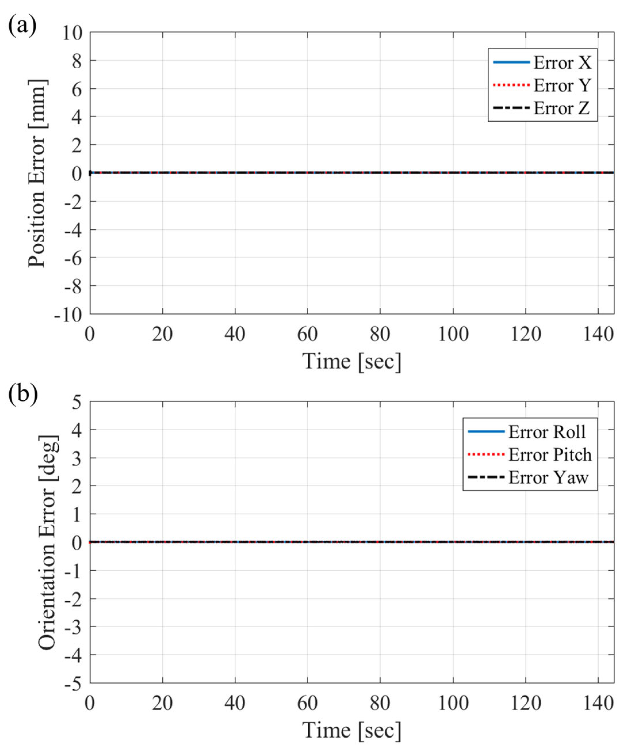
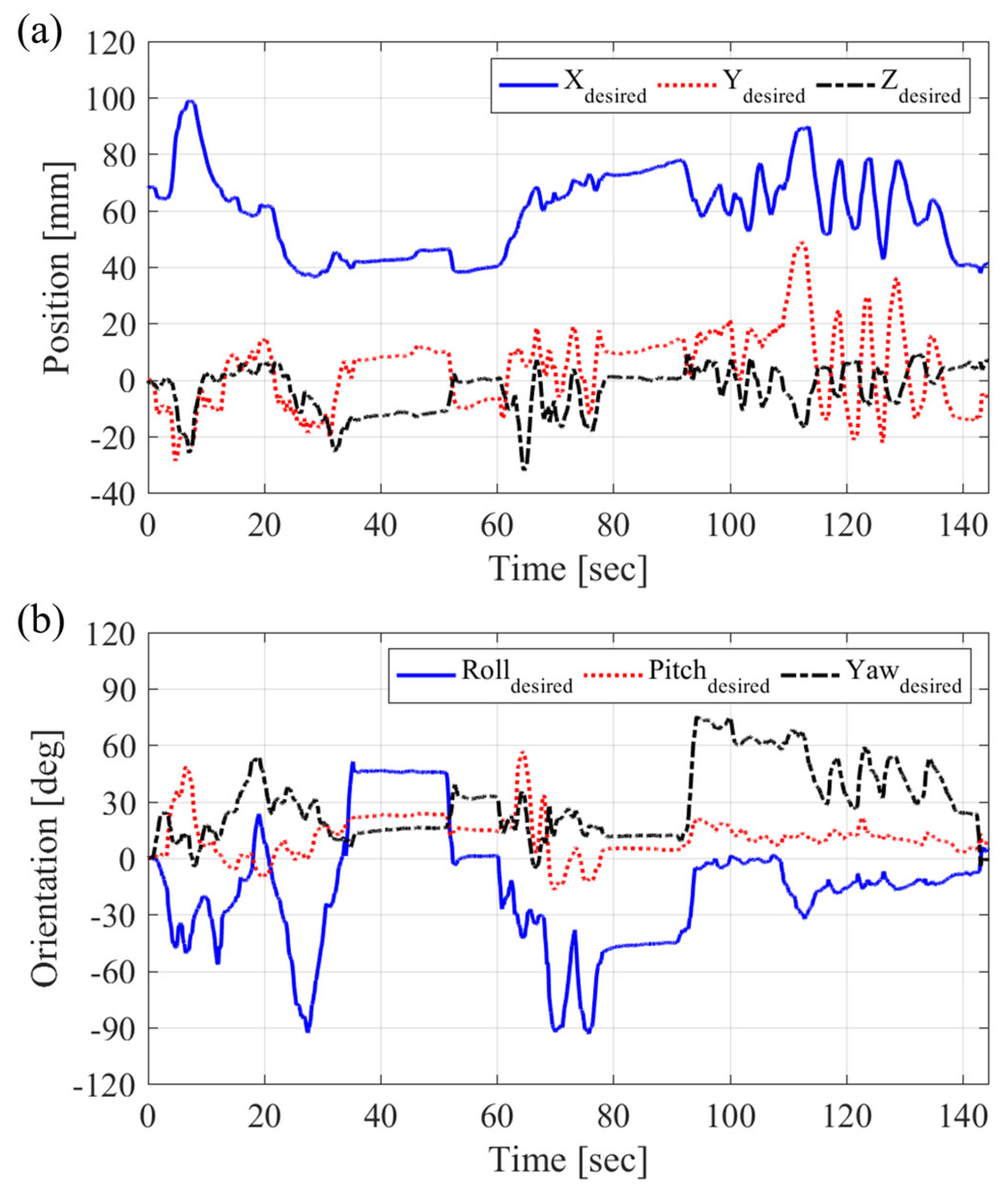
Measurements were performed with an electromagnetic (EM) tracking system (Aurora, Northern Digital Inc., Canada). The field generator was set up around the robot arm, and six-DoF sensors were attached to the tip of the robot arm and the reference points, as shown in Figure 20. The position accuracy was 0.48 mm with a 95% confidential interval of 0.88 mm, and the orientation accuracy was 0.30° with a 95% confidential interval of 0.48°. The actual motion of the robot driven through the path generators was measured according to the desired path. The same desired path as in Figure 11 was applied to the system. The control group was the motion that was operated by the path generator based on the constant-curvature model of the arm configuration and wire length. The articulated robotic arm was simplified as the constant-curvature model. The driving wire length was generated symmetrically based on the curvature model.

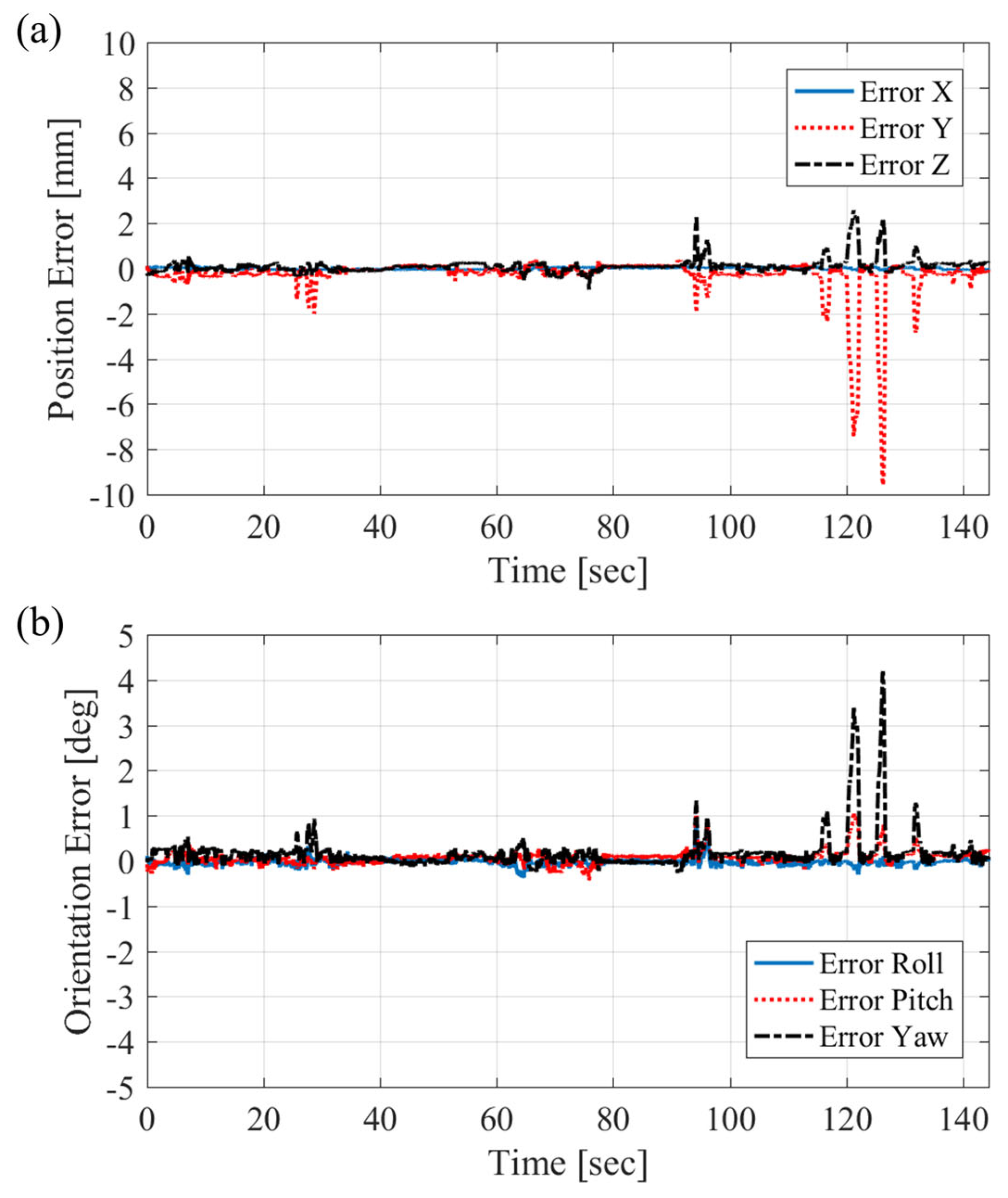
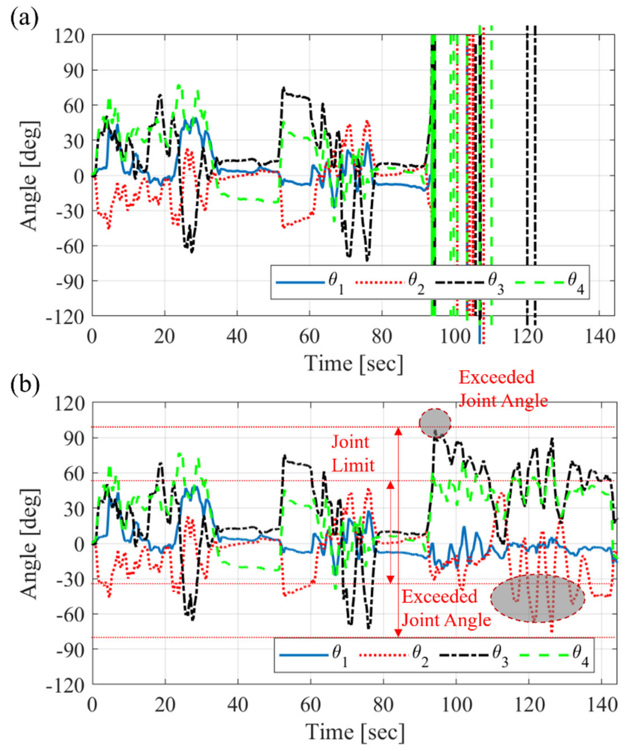
The motions of the end-effector controlled with the two proposed path generators followed the desired trajectory well, but the motion with the constant-curvature model did not, as shown in Figure 21. The blue solid line presents the end-effector’s orientation with the optimization path generator, and the green dotted line shows the results from the path generator with the Jacobian matrix and PID control algorithm. The red dashed–dotted line represents the results from the constant-curvature model, and the black dashed line is the desired orientation path. The two proposed path generators showed similar results, even near 120 s. Both of the experimental results with the two path generators could not reach the desired values due to the physical limitation of the joint structure. However, the path generator with the Jacobian matrix and PID control algorithm generated commands that were beyond the limitations of the joint structure. If these commands are repeated, the wires and joints may suffer damage.

The experimental results showed the accuracy of the proposed kinematic model and the validity of the two path generator algorithms. The forward kinematic model of the articulated joint robot arm with frame transformation and the symmetric wire length model for the joint structure were more precise than the constant-curvature model. The two proposed path generators solved the inverse kinematics efficiently and generated accurate actuation paths for open-loop control in an actual system.

6. Conclusions

A wire-driven surgical robot arm with a joint structure has a tiny structure and operates inside the human body. In general, the robot is operated through open-loop control. Furthermore, the robot has to operate according to an arbitrary path in real-time and not a predefined path. A path generator based on an accurate kinematic model is vital to the performance of the robot. In this study, the accuracy of the kinematic model was improved with the product of the transformation matrices with moving frames and an asymmetrical wire-driving model for the joint structure. The proposed wire-driving model also solved the coupling problem due to the double-segment structure for single-port surgery.

This paper presented two path generators that solved for inverse kinematics: an optimization path generator and a path generator with a Jacobian matrix and PID control algorithm. The optimization path generator solved the inverse kinematics using the SQP numerical optimization method. This path generator operated within a computing loop time of the 10 ms. Operators did not feel the delay, but considering that additional algorithms will be implemented, the computational time due to iteration may be worrisome. The logic of constraints on the mechanical limits of robot arms worked well in real-time even when the master device generated the desired position and direction at an excessive value.

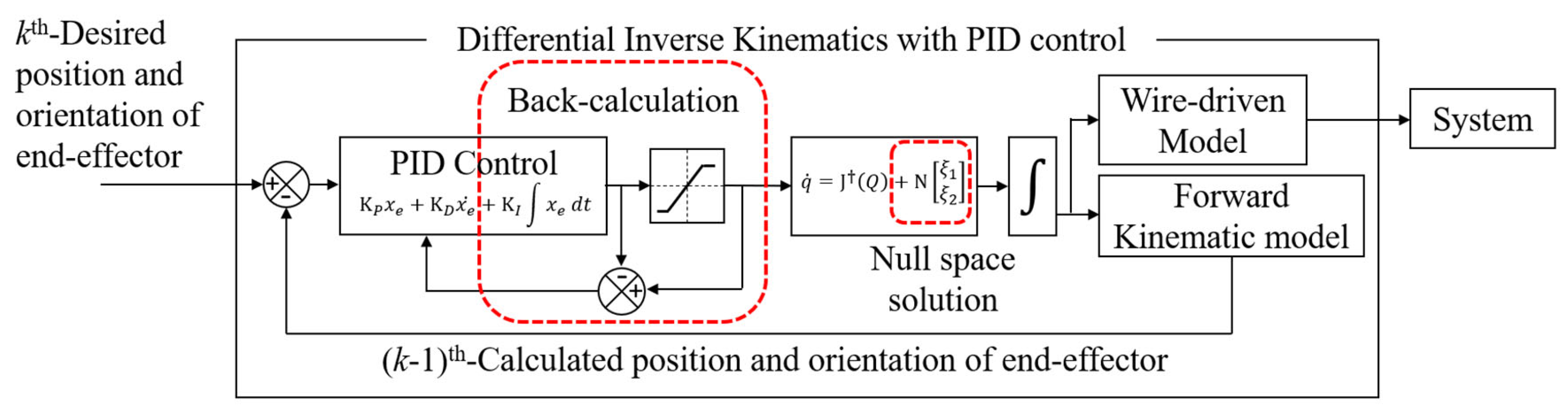
The path generator with the Jacobian matirx and PID control algorithm derived the inverse kinematic solution using differential kinematics and a feedback control algorithm. The important features, in this case, were the null space solution for the coupled constraints due to the articulated joint structure and back-calculation to prevent sudden divergence. This path generator was much faster and much more accurate than the optimization path generator. However, it could not restrict the actuation value to the mechanical limits. The experimental results showed performance improvement due to the accurate kinematic model and the validity of the path generators embedded in a surgical robot prototype. In future work, a path-regulation algorithm will be designed for a second path generator.

References

1. Bergeles, C.; Yang, G. From passive tool holders to microsurgeons: Safer, smaller, smarter surgical robots. IEEE Trans. Biomed. Eng. 2014, 61, 1565–1576. [Google Scholar] [CrossRef]
2. Turchetti, G.; Palla, I.; Pierotti, F.; Cuschieri, A. Economic evaluation of da Vinci-assisted robotic surgery: A systematic review. Surg. Endosc. 2012, 26, 598–606. [Google Scholar] [CrossRef] [PubMed]
3. Maeso, S.; Reza, M.; Mayol, J.A.; Blasco, J.A.; Guerra, M.; Andradas, E.; Plana, M.N. Efficacy of the Da Vinci surgical system in abdominal surgery compared with that of laparoscopy: A systematic review and meta-analysis. Ann. Surg. 2010, 252, 254–262. [Google Scholar] [CrossRef] [PubMed]
4. Kroh, M.; El-Hayek, K.; Rosenblatt, S.; Chand, B.; Escobar, P.; Kaouk, J.; Chalikonda, S. First human surgery with a novel single-port robotic system: Cholecystectomy using the da Vinci Single-Site platform. Surg. Endosc. 2011, 25, 3566–3573. [Google Scholar] [CrossRef] [PubMed]
5. Maurice, M.J.; Ramirez, D.; Kaouk, H.H. Robotic laparoscopic single-site retroperitioneal renal surgery: Initial investigation of a purpose-built single-port surgical system. Eur. Urol. 2017, 71, 643–647. [Google Scholar] [CrossRef]
6. Zhao, J.; Feng, B.; Zheng, M.H.; Xu, K. Surgical robots for SPL and NOTES: A review. Minim. Invasive Ther. Allied Technol. 2015, 25, 8–17. [Google Scholar] [CrossRef]
7. Zorn, L.; Nageotte, F.; Zanne, P.; Legner, A.; Dallemagne, B.; Marescaux, J.; Mathelin, M. A novel telemanipulated robotic assistant for surgical endoscopy: Preclinical application to ESD. IEEE Trans. Biomed. Eng. 2018, 65, 797–808. [Google Scholar] [CrossRef] [PubMed]
8. Conrad, B.L.; Zinn, M.R. Interleaved continuum-rigid manipulation: An approach to increase the capability of minimally invasive surgical systems. IEEE/ASME Trans. Mechatron. 2017, 22, 29–40. [Google Scholar] [CrossRef]
9. Jelínek, F.; Arkenbout, A.E.; Henselmans, W.J.P.; Pessers, R.; Breedveld, P. Classification of joints used in steerable instruments for minimally invasive surgery-a review of the state of the art. J. Med. Devices 2015, 9, 010801-1–010801-11. [Google Scholar]
10. Chikhaoui, M.T.; Lilge, S.; Kleinschmidt, S.; Burgner-Kahrs, J. Comparison of modeling approaches for a tendon actuated continuum robot with three extensible segments. IEEE Robot. Autom. Lett. 2019, 4, 989–996. [Google Scholar] [CrossRef]
11. Webster, R.J.; Jones, B.A. Design and kinematic modeling of constant curvature continuum robots: A review. Int. J. Robot. Res. 2010, 29, 1661–1683. [Google Scholar] [CrossRef]
12. Mahl, T.; Hildebrandt, A.; Sawodny, O. A variable curvature kinematics for kinematic control of the bionic handling assistant. IEEE Trans. Robot. 2014, 30, 935–949. [Google Scholar] [CrossRef]
13. Godage, I.S.; Medrano-Cerda, G.A.; Branson, D.T.; Guglielmino, E.; Caldwell, D.G. Modal kinematics for multisection continuum arms. Bioinspiration Biomim. 2015, 10, 035002-1–035002-20. [Google Scholar] [CrossRef] [PubMed]
14. Jones, B.A.; Walker, I.D. Practical kinematics for real-time implementation of continuum robots. IEEE Trans. Robot. 2006, 22, 1087–1099. [Google Scholar] [CrossRef]
15. Boggs, P.T.; Tolle, J.W. Sequential quadratic programming for large-scale nonlinear optimization. J. Comput. Appl. Math. 2000, 124, 123–137. [Google Scholar] [CrossRef]
16. Xu, J.; Wang, W.; Sun, Y. Two optimization algorithms for solving robotics inverse kinematics with redundancy. J. Control Theory Appl. 2010, 8, 166–175. [Google Scholar] [CrossRef]
17. Beeson, P.; Ames, B. TRAC-IK: An open-source library for improved solving of generic inverse kinematics. In Proceedings of the IEEE-RAS International Conference on Humanoid Robots, Seoul, South Korea, 3–5 November 2015; pp. 928–935. [Google Scholar]
18. Falco, P.; Natale, C. On the stability of closed-loop inverse kinematics algorithms for redundant robots. IEEE Trans. Robot. 2011, 27, 780–784. [Google Scholar] [CrossRef]
19. Colomé, A.; Torras, C. Closed-loop inverse kinematics for redundant robots: Comparative assessment and two enhancements. IEEE/ASME Trans. Mechatron. 2015, 20, 944–955. [Google Scholar]
20. Suh, J.W. Cable-Driven Pulleyless Rolling Joint with Elastic Fixtures for Medical Applications. Ph.D. Thesis, School of Mechanical, Aerospace and Systems Engineering, KAIST, Daejeon, South Korea, 2013. [Google Scholar]
21. Kim, L.H.; Bargar, C.; Che, Y.; Okamura, A.M. Effects of master-salve tool misalignment in a teleoperated surgical robot. In Proceedings of the IEEE International Conference on Robotics and Automation (ICRA), Seattle, WA, USA, 26–30 May 2015; pp. 5364–5370. [Google Scholar]
22. Coevoet, E.; Escande, A.; Duriez, C. Optimization-based inverse model of soft robots with contact handling. IEEE Robot. Autom. Lett. 2017, 2, 1413–1419. [Google Scholar] [CrossRef]
23. Li, M.; Kang, R.; Geng, S.; Guglielmino, E. Design and control of a tendon-driven continuum robot. Trans. Inst. Meas. Control 2017, 40, 0142331216685607. [Google Scholar] [CrossRef]
24. Berthet-Rayne, P.; Leibrandt, K.; Gras, G.; Fraisse, P.; Crosnier, A.; Yang, G.Z. Inverse kinematics control methods for redundant snake-like robot teleoperation during minimally invasive surgery. IEEE Robot. Autom. Lett. 2018, 3, 2501–2508. [Google Scholar] [CrossRef]
25. Spong, M.W.; Hutchinson, S.; Vidyasagar, M. Robot Modeling and Control, 1st ed.; John Wiley & Sons, Inc.: New York, NY, USA, 2006; pp. 113–130. [Google Scholar]
26. Huang, C.; Peng, X. Output-feedback PID controller for robot manipulators with Jacobian uncertainty. In Proceedings of the International Conference on Intelligent Systems Design and Applications, Kaohsiung, Taiwan, 26–28 November 2008; pp. 329–334. [Google Scholar]
27. Huang, C.; Peng, X. Dynamic analysis and closed-loop control of biological cells in transportation using robotic manipulation system with optical tweezers. In Proceedings of the IEEE Conference on Automation Science and Engineering (CASE), Toronto, ON, Canada, 21–24 August 2010; pp. 240–245. [Google Scholar]
28. Chan, T.F.; Dubey, R.V. A weighted least-norm solution based scheme for avoiding joint limits for redundant joint manipulators. IEEE Trans. Robot. Autom. 1995, 11, 286–292. [Google Scholar] [CrossRef]
29. Huang, S.; Peng, Y.; Wei, W.; Xiang, J. Clamping weighted least-norm method for the manipulator kinematic control: Avoiding joint limits. In Proceedings of the 33rd Chinese Control Conference, Nanjing, China, 28–30 July 2014; pp. 8309–8314. [Google Scholar]
30. Huynh, D.Q. Metrics for 3D rotations: Comparison and analysis. J. Math. Imaging Vis. 2009, 35, 155–164. [Google Scholar] [CrossRef]
Figure 1. Wire-driven surgical robot with joint structure: (a) suturing test of prototype; (b) conceptual diagram of working principle.
Applsci 09 04114 g001
Figure 2. Structure of snake-like surgical robotic arms: (a) single segment with slit structure; (b) single segment with joint structure; (c) double segment with joint structure.
Applsci 09 04114 g002
Figure 3. Relation between three spaces of kinematics of wire-driven robotic arm.
Applsci 09 04114 g003
Figure 4. Diagram of a single-joint section.
Applsci 09 04114 g004
Figure 5. Articulated joints robotic arm with double segments.
Applsci 09 04114 g005
Figure 6. Comparison of forward kinematics between curvature model and joint model: (a) curvature model; (b) joint model; (c) position difference; (d) orientation difference.
Applsci 09 04114 g006
Figure 7. Diagram of wire length in a single joint: (a) conventional curvature model; (b) modified model with joint structure.
Applsci 09 04114 g007
Figure 8. Comparison of driving wire length between curvature model and joint model.
Applsci 09 04114 g008
Figure 9. Distal section views of robotic arm and wire assignment.
Applsci 09 04114 g009
Figure 10. Block diagram of the open-loop control via the optimization path generator.
Applsci 09 04114 g010
Figure 11. Desired position and orientation of end-effector of robot arm, which is recorded by the haptic master device, as it simulates a suturing motion: (a) position; (b) orientation.
Applsci 09 04114 g011
Figure 12. Actuation value for the desired six-DoF motion from the optimization path generator: (a) joint angles of robot arm; (b) translation stroke and rotation angle of the whole body.
Applsci 09 04114 g012
Figure 13. Error of the optimization path generator: (a) position error; (b) orientation error.
Applsci 09 04114 g013
Figure 14. Driving wire length from the optimization path generator for (a) proximal joins and (b) distal joints.
Applsci 09 04114 g014
Figure 15. Block diagram of the open-loop control via the path generator to solve the differential inverse kinematics with the PID control algorithm.
Applsci 09 04114 g015
Figure 16. Inverse kinematic solution of distal coupled joint angles with the constraint algorithm using the null space solution.
Applsci 09 04114 g016
Figure 17. Inverse kinematic solution (a) without back-calculation and (b) with back-calculation.
Applsci 09 04114 g017
Figure 18. Error of the path generator with the Jacobian matrix and PID control algorithm: (a) position error and (b) orientation error.
Applsci 09 04114 g018
Figure 19. Driving wire length from the path generator with the Jacobian matrix and PID control algorithm for (a) proximal joints and (b) distal joints.
Applsci 09 04114 g019
Figure 20. Experimental apparatus.
Applsci 09 04114 g020
Figure 21. Experimental results of the end-effector’s orientation under the proposed path generators with the kinematic model and the constant curvature model: (a) roll; (b) pitch; (c) yaw.
Applsci 09 04114 g021