Figure 1.
The flowchart of the algorithm.
Figure 1.
The flowchart of the algorithm.
Figure 2.
n-DOF structure model.
Figure 2.
n-DOF structure model.
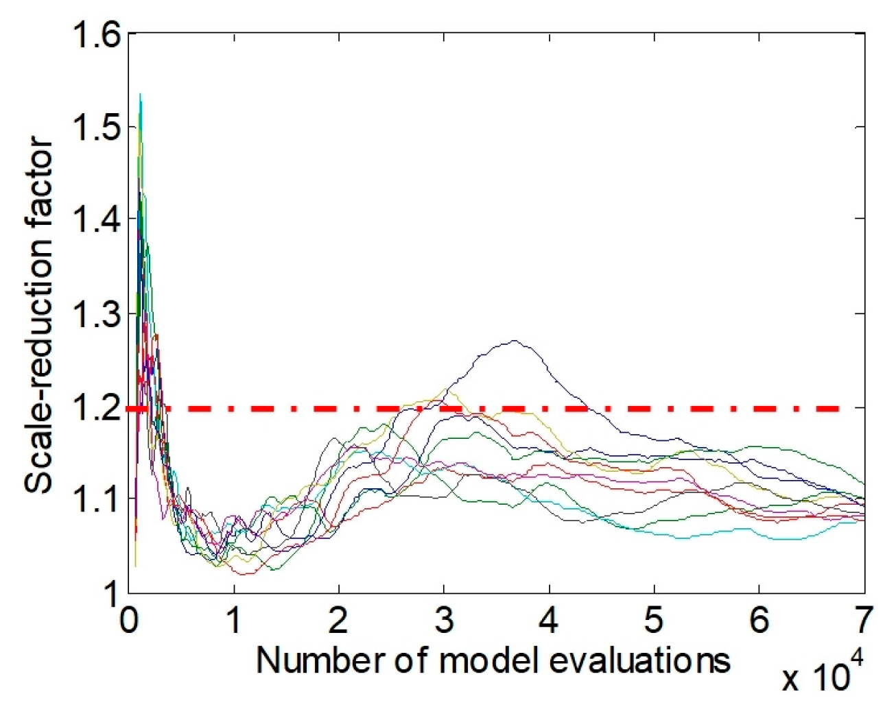
Figure 3.
Evolution of the scale reduction factor for the eight estimation parameters: (a) Case 1: 0% noise + Full Outputs; (b) Case 2: 10% noise + Full Outputs; (c) Case 3: 10% noise + Partial Outputs.
Figure 3.
Evolution of the scale reduction factor for the eight estimation parameters: (a) Case 1: 0% noise + Full Outputs; (b) Case 2: 10% noise + Full Outputs; (c) Case 3: 10% noise + Partial Outputs.
Figure 4.
Generated samples for the three estimation parameters (k1, k5, ζ1): (a) Case 1: 0% noise + Full Outputs; (b) Case 2: 10% noise + Full Outputs; (c) Case 3: 10% noise + Partial Outputs.
Figure 4.
Generated samples for the three estimation parameters (k1, k5, ζ1): (a) Case 1: 0% noise + Full Outputs; (b) Case 2: 10% noise + Full Outputs; (c) Case 3: 10% noise + Partial Outputs.
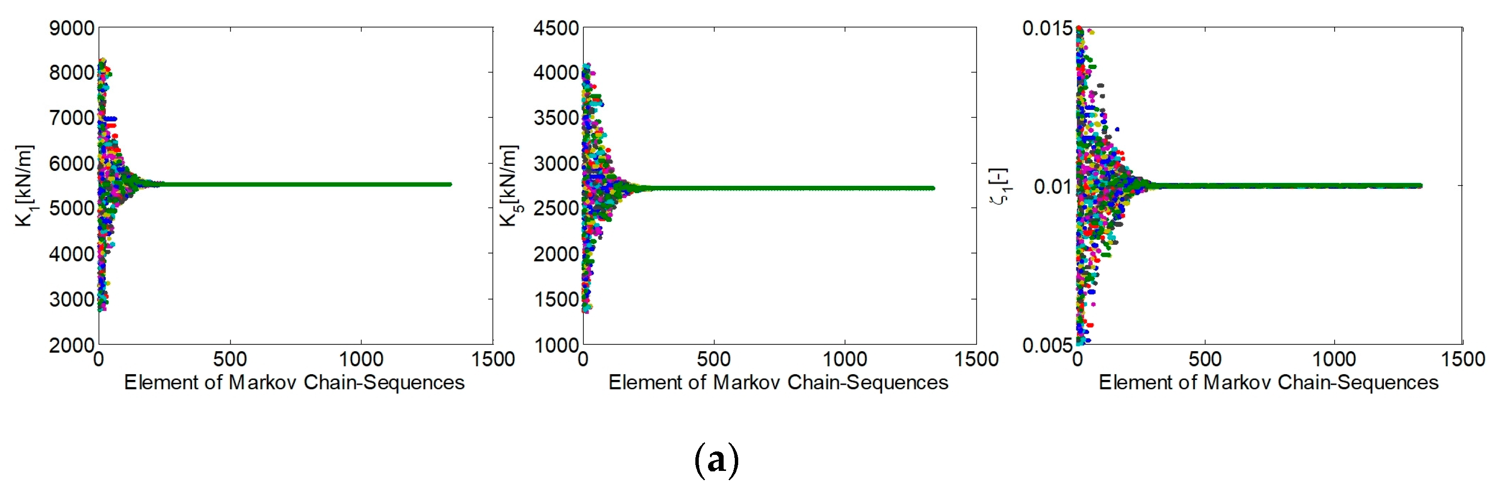
Figure 5.
Marginal posterior probability distributions of the three estimation parameters (k1, k5, ζ1): (a) Case 1: 0% noise + Full Outputs; (b) Case 2: 10% noise + Full Outputs; (c) Case 3: 10% noise + Partial Outputs.
Figure 5.
Marginal posterior probability distributions of the three estimation parameters (k1, k5, ζ1): (a) Case 1: 0% noise + Full Outputs; (b) Case 2: 10% noise + Full Outputs; (c) Case 3: 10% noise + Partial Outputs.
Figure 6.
Evolution of the scale reduction factor for the estimation parameters.
Figure 6.
Evolution of the scale reduction factor for the estimation parameters.
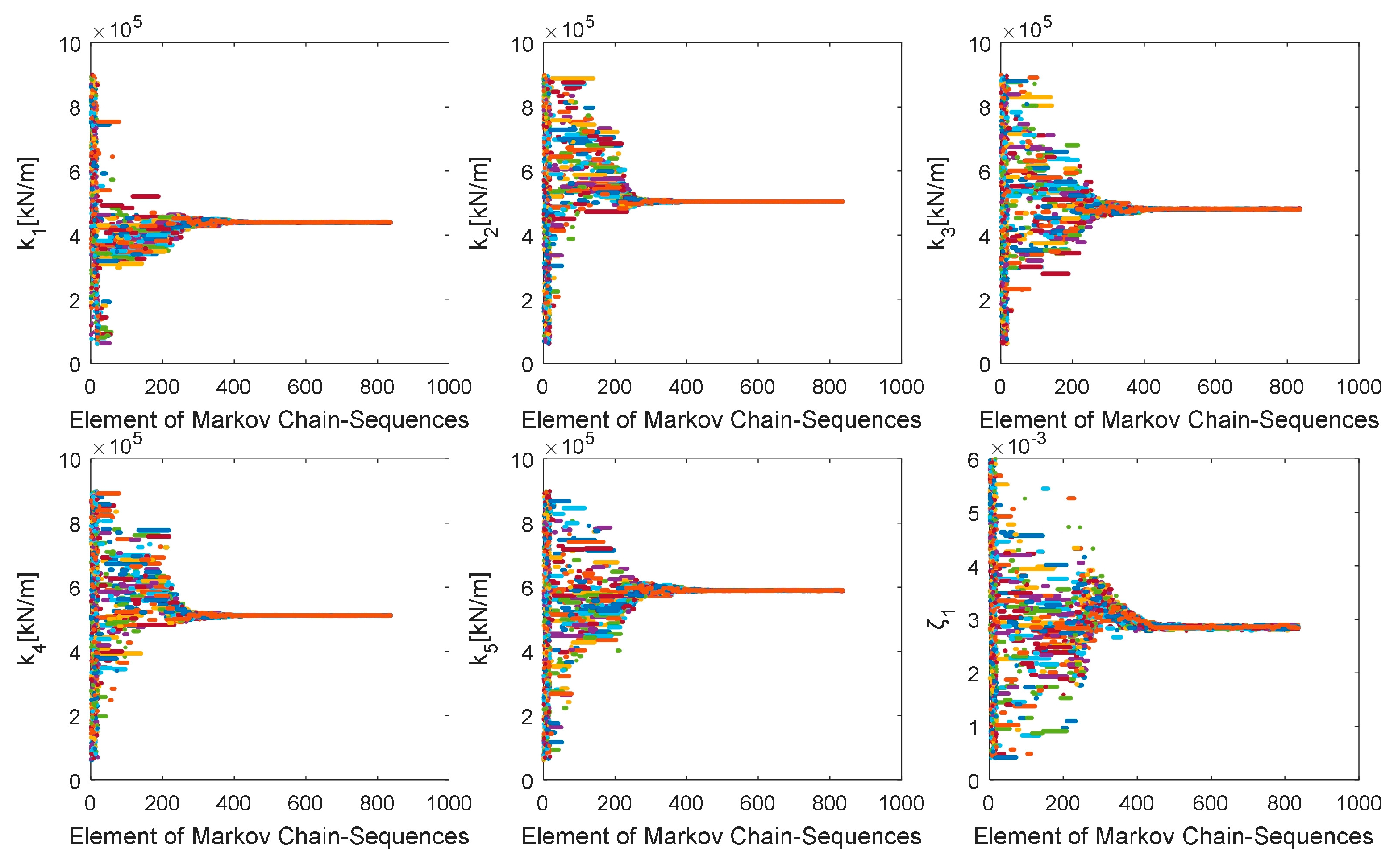
Figure 7.
Generated samples for the six estimation parameters (k1, k6, k9, m1, m6, ζ1).
Figure 7.
Generated samples for the six estimation parameters (k1, k6, k9, m1, m6, ζ1).
Figure 8.
Marginal posterior probability distributions of the six estimation parameters (k1, k6, k9, m1, m6, ζ1).
Figure 8.
Marginal posterior probability distributions of the six estimation parameters (k1, k6, k9, m1, m6, ζ1).
Figure 9.
Schematic diagram and the test model of the 5-DOF structure system.
Figure 9.
Schematic diagram and the test model of the 5-DOF structure system.
Figure 10.
Evolution of the scale reduction factor for the seven estimation parameters.
Figure 10.
Evolution of the scale reduction factor for the seven estimation parameters.
Figure 11.
Generated samples for the six estimation parameters (k1, k2, k3, k4, k5, ζ1).
Figure 11.
Generated samples for the six estimation parameters (k1, k2, k3, k4, k5, ζ1).
Figure 12.
Marginal posterior probability distributions of the six estimation parameters (k1, k2, k3, k4, k5, ζ1).
Figure 12.
Marginal posterior probability distributions of the six estimation parameters (k1, k2, k3, k4, k5, ζ1).
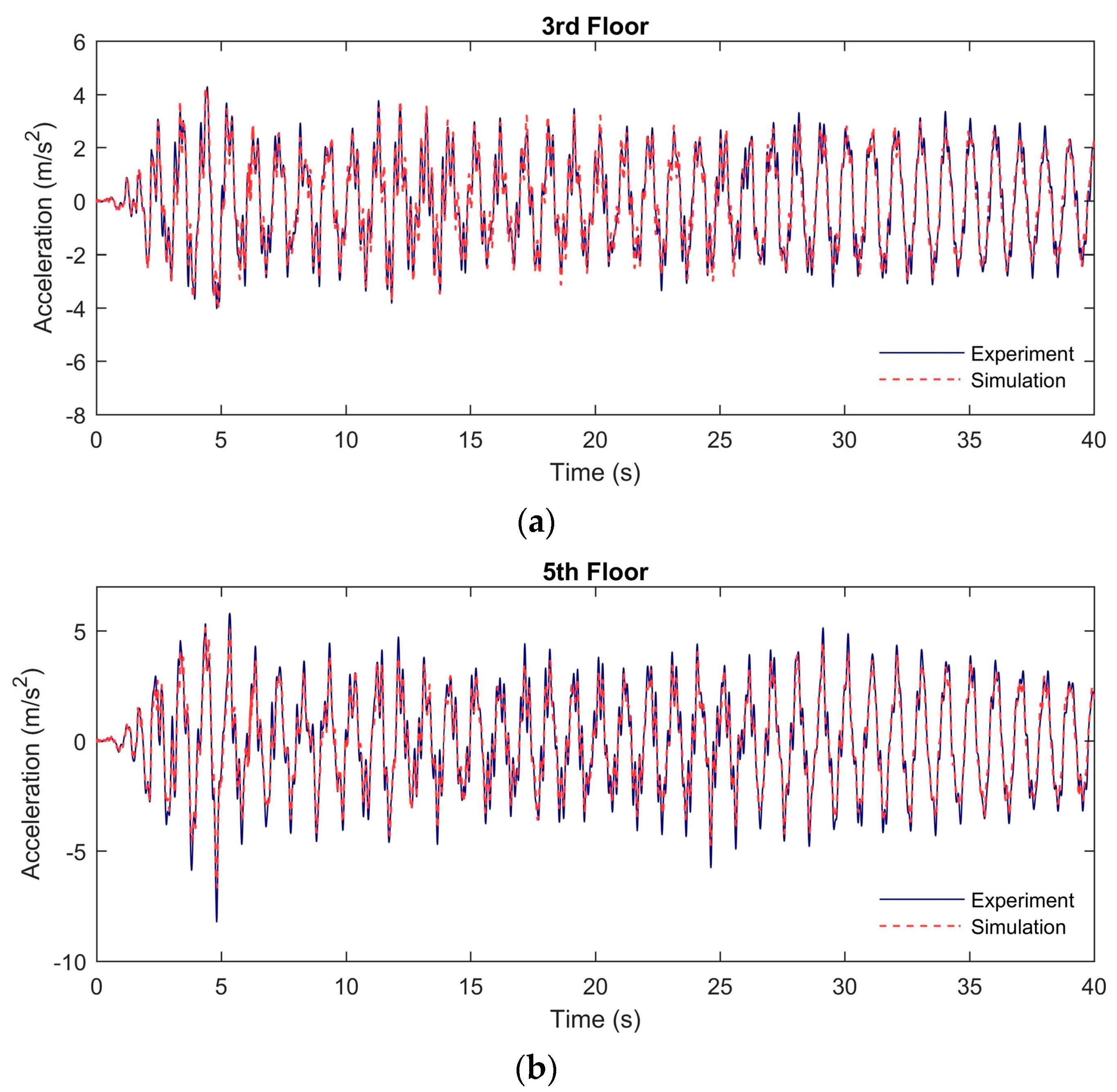
Figure 13.
Experimental and simulation acceleration time histories in the linear structural system: (a) At the 3rd floor; (b) At the 5th floor.
Figure 13.
Experimental and simulation acceleration time histories in the linear structural system: (a) At the 3rd floor; (b) At the 5th floor.
Figure 14.
Experimental and simulation acceleration time histories in the linear structural system: (a) At the 3rd floor; (b) At the 5th floor.
Figure 14.
Experimental and simulation acceleration time histories in the linear structural system: (a) At the 3rd floor; (b) At the 5th floor.
Figure 15.
The test model and a simplified schematic of the system.
Figure 15.
The test model and a simplified schematic of the system.
Figure 16.
Evolution of the scale reduction factor for the 11 estimation parameters.
Figure 16.
Evolution of the scale reduction factor for the 11 estimation parameters.
Figure 17.
Generated samples for the six estimation parameters (k1, k3, k5, ζ1, ωp, ζc).
Figure 17.
Generated samples for the six estimation parameters (k1, k3, k5, ζ1, ωp, ζc).
Figure 18.
Marginal posterior probability distributions of the six estimation parameters (k1, k3, k5, ζ1, ωp, ζc).
Figure 18.
Marginal posterior probability distributions of the six estimation parameters (k1, k3, k5, ζ1, ωp, ζc).
Figure 19.
Experimental and simulation acceleration time histories in the nonlinear structural system: (a) At the 3rd floor; (b) At the 5th floor.
Figure 19.
Experimental and simulation acceleration time histories in the nonlinear structural system: (a) At the 3rd floor; (b) At the 5th floor.
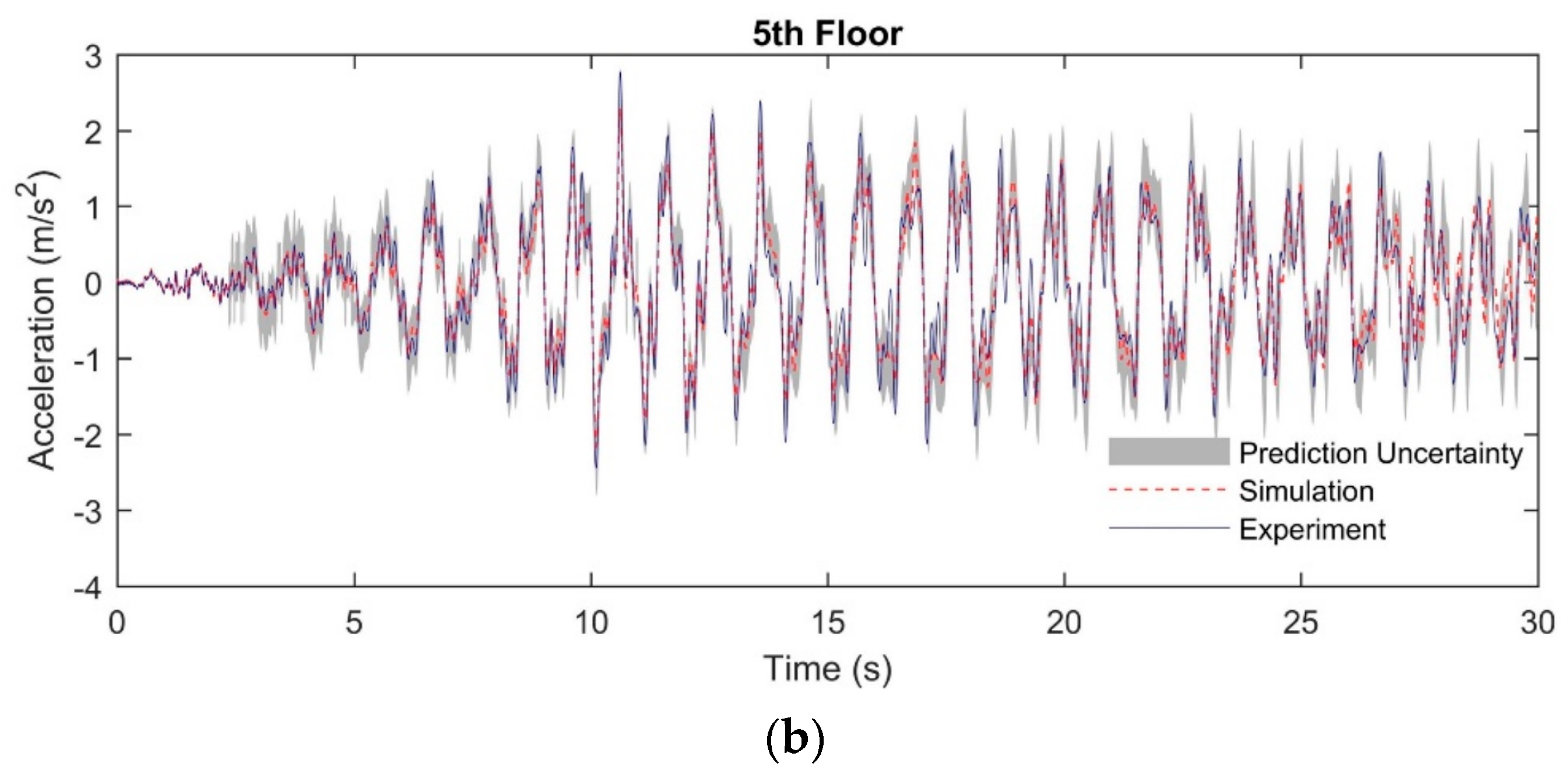
Figure 20.
Prediction uncertainty ranges of acceleration histories in the nonlinear structural system: (a) At the 3rd floor; (b) At the 5th floor.
Figure 20.
Prediction uncertainty ranges of acceleration histories in the nonlinear structural system: (a) At the 3rd floor; (b) At the 5th floor.
Table 1.
Structure properties of the 8-DOF system.
Table 1.
Structure properties of the 8-DOF system.
| Mass (kg) | |
|---|
| m1~m7 | 4.95 |
| m8 | 4.51 |
| Stiffness (kN/m) | |
| k1 | 5.53 × 10³ |
| k2~k8 | 2.72 × 10³ |
| Damping ratio | |
| ζ1 | 1 × 10⁻² |
| ζ2 | 3 × 10⁻² |
Table 2.
Bounds of the prior uniform parameter distributions.
Table 2.
Bounds of the prior uniform parameter distributions.
| Parameter | Lower Bound | Upper Bound |
|---|
| k1 (kN/m) | 2.765 × 10³ | 11.06 × 10³ |
| k2~k8 (kN/m) | 1.36 × 10³ | 5.44 × 10³ |
| ζ1 | 5 × 10⁻¹ | 2 × 10⁻² |
| ζ2 | 1.5 × 10⁻² | 6 × 10⁻² |
Table 3.
Statistics of the posterior parameter distribution with the relative error (R.E.) between the posterior mean and the true value, including the standard deviation (S.D.) for each scenario.
Table 3.
Statistics of the posterior parameter distribution with the relative error (R.E.) between the posterior mean and the true value, including the standard deviation (S.D.) for each scenario.
| Parameter | S.D. | R.E |
|---|
| Case1 | Case2 | Case3 | Case1 | Case2 | Case3 |
|---|
| k1 (kN/m) | 0 | 8.81 | 25.5 | 0% | 0.16% | 0.30% |
| k2 (kN/m) | 0 | 4.39 | 9.55 | 0% | 0.16% | 0.35% |
| k3 (kN/m) | 0 | 3.6 | 8.72 | 0% | 0.13% | 0.32% |
| k4 (kN/m) | 0 | 4.27 | 6.56 | 0% | 0.16% | 0.24% |
| k5 (kN/m) | 0 | 7.49 | 1.51 | 0% | 0.28% | 0.42% |
| k6 (kN/m) | 0 | 4.56 | 7.3 | 0% | 0.17% | 0.28% |
| k7 (kN/m) | 0 | 5.44 | 8.81 | 0% | 0.20% | 0.32% |
| k8 (kN/m) | 0 | 6.37 | 10.3 | 0% | 0.23% | 0.38% |
| ζ1 | 0 | 1.64 × 10⁻⁴ | 2.63 × 10⁻⁴ | 0% | 1.64% | 2.63% |
| ζ2 | 0 | 5.8 × 10⁻⁵ | 1.09 × 10⁻⁴ | 0% | 0.49% | 0.76% |
Table 4.
Structure properties of the 10-DOF system.
Table 4.
Structure properties of the 10-DOF system.
| Mass (kg) | |
|---|
| m1~m4 | 6000 |
| m5~m8 | 4200 |
| Stiffness (kN/m) | |
| k1~k4 | 5000 |
| k5~k8 | 4000 |
| k9~k10 | 3000 |
| Stiffness (kN/m) | |
| First mode | 1.321 |
| Second mode | 0.505 |
Table 5.
Average error (avg. error) and maximum error (max. error) between the parameter value found with the lowest posterior probability and the true value.
Table 5.
Average error (avg. error) and maximum error (max. error) between the parameter value found with the lowest posterior probability and the true value.
| Parameter | GA | PSO | BB-BC | SCE-UA | SCEM-UA |
|---|
| Avg. error—m (%) | 2.98 | 2.74 | 2.61 | 1.04 | 0.68 |
| Max. error—m (%) | 6.62 | 7.11 | 4.55 | 3.17 | 1.49 |
| Avg. error—k (%) | 3.00 | 3.00 | 2.25 | 1.12 | 0.73 |
| Max. error—k (%) | 6.81 | 6.10 | 3.33 | 2.62 | 1.52 |
| Avg. error—c (%) | 8.41 | 7.96 | 2.79 | 2.94 | 2.71 |
| Max. error—c (%) | 15.29 | 10.7 | 4.72 | 6.13 | 5.40 |
Table 6.
Bounds of the prior uniform distributions for the parameters of the 5-DOF model.
Table 6.
Bounds of the prior uniform distributions for the parameters of the 5-DOF model.
| Parameter | Lower Bound | Upper Bound |
|---|
| k1~k5 (kN/m) | 6.1 × 10⁴ | 9.07 × 10⁵ |
| ζ1 | 4 × 10⁻⁴ | 6 × 10⁻³ |
| ζ2 | 1 × 10⁻⁴ | 1.5 × 10⁻³ |
Table 7.
Summarizing statistics of the posterior parameter distribution mean value (M.V., standard deviation (S.D.), and relative deviation (R.E.)).
Table 7.
Summarizing statistics of the posterior parameter distribution mean value (M.V., standard deviation (S.D.), and relative deviation (R.E.)).
| Parameter | M.V. | S.D. | R.D. |
|---|
| k1 (kN/m) | 4.434 × 10⁵ | 2.52 × 10² | 0.057% |
| k2 (kN/m) | 5.034 × 10⁵ | 96.8 | 0.019% |
| k3 (kN/m) | 4.755 × 10⁵ | 3.65 × 10² | 0.077% |
| k4 (kN/m) | 5.107 × 10⁵ | 1.73 × 10² | 0.034% |
| k5 (kN/m) | 5.980 × 10⁵ | 3.75 × 10² | 0.063% |
| ζ1 | 2.5 × 10⁻³ | 2.58 × 10⁻⁶ | 0.10% |
| ζ2 | 8.59 × 10⁻⁴ | 1.18 × 10⁻⁶ | 0.14% |
Table 8.
Bounds of the prior uniform distributions for the parameters of the nonlinear structural system.
Table 8.
Bounds of the prior uniform distributions for the parameters of the nonlinear structural system.
| Parameter | Lower Bound | Upper Bound |
|---|
| k1~k5 (kN/m) | 1 × 10⁵ | 1 × 10⁶ |
| ζ1 | 1.5 × 10⁻⁵ | 7.5 × 10⁻³ |
| ζ2 | 5 × 10⁻⁶ | 2.5 × 10⁻³ |
| ωc (rad/s) | 5 × 10⁻² | 25 |
| ωp (rad/s) | 1 | 5 × 10² |
| ζc | 1 × 10⁻³ | 5 × 10⁻¹ |
| ζp | 2 × 10⁻³ | 1.0 |
Table 9.
Summarizing statistics of the posterior parameter distribution (Mean Value (M.V.), Standard Deviation (S.D.), and Relative Deviation (R.E.)).
Table 9.
Summarizing statistics of the posterior parameter distribution (Mean Value (M.V.), Standard Deviation (S.D.), and Relative Deviation (R.E.)).
| Parameter | M.V. | S.D. | R.D. |
|---|
| k1 (kN/m) | 5.011 × 10⁵ | 7.73 × 10³ | 1.54% |
| k2 (kN/m) | 5.619 × 10⁵ | 4.45 × 10³ | 0.79% |
| k3 (kN/m) | 4.879 × 10⁵ | 6.98 × 10³ | 1.43% |
| k4 (kN/m) | 4.721 × 10⁵ | 5.61 × 10³ | 1.19% |
| k5 (kN/m) | 5.190 × 10⁵ | 4.93 × 10³ | 0.95% |
| ζ1 | 4.423 × 10⁻³ | 3.11 × 10⁻⁵ | 0.70% |
| ζ2 | 6.601 × 10⁻⁴ | 3.79 × 10⁻⁶ | 0.57% |
| ωc (rad·s) | 1.584 × 10² | 2.3 × 10⁻¹ | 1.45% |
| ωp (rad·s) | 1.14 × 10² | 4.94 | 4.33% |
| ζc | 3.175 × 10⁻¹ | 2.38 × 10⁻³ | 0.75% |
| ζp | 2.621 × 10⁻¹ | 1 × 10⁻² | 3.81% |


