FDCNet: Frontend-Backend Fusion Dilated Network Through Channel-Attention Mechanism

Abstract

Crowd counting has attracted much attention in computer vision owing to its fundamental contribution in public security. But due to occlusions, perspective distortions, scale variations, and background interference it faces a great challenge. In this paper we propose a novel model to count crowds, named FDCNet: frontend-backend fusion dilated network through channel-attention mechanism. It merges the frontend feature map with the backend feature map, achieving a fusion of various scale features without additional branches or extra subtasks. The fusion is fed into the channel-attention block to optimize the procedure and to conduct feature recalibration to use global and spatial information. Furthermore, we utilize dilated layers to obtain a high-quality density map, and the SSIM-based loss function is added to compare the local correlation between the estimated density map and the ground truth. Our FDCNet is verified in four common datasets and gets a brilliant estimation.

1. Introduction

In recent years, with the rapid development of living standards and transportation, there has been a dramatic improvement in crowd counting. It plays a critical role in the maintenance of public security. For instance, in the congested scene, the monitoring device can real-time monitor the change of crowd to prevent overcrowding and abnormal conditions. Whereas the task suffers from occlusions, perspective distortions, scale variations, and background interference. It immensely remains a challenge to reach remarkable accuracy on the prediction of crowd counting in a single image.

Extensive studies and a mountain of efforts have been attempted. There has been considerable progress in crowd counting. Early works detected each individual pedestrian in a crowd scene [1], or used multiple handcrafted features to regress the number of persons [2]. But they got trouble in detecting pedestrians in congested scenes caused by severe occlusions. Nowadays, mainstream works aim to generate crowd density maps instead of counting persons directly to alleviate the occlusions. Furthermore, density maps also contain spatial information, which can be better applied in public security. GAN- based [3,4] and CNN-based [5,6,7,8,9,10,11,12,13,14,15,16] methods have achieved excellent improvements.

Due to the different distances from the surveillance camera and perspective problems, there are persons with unequal sizes of head in a single image. Hence, the biggest conundrum is the scale diversity, which restrains the counting accuracy. Some works [5,6,7,8,9] use multi-scale architecture with different convolutional kernels to address the scale variation, while some works [10,11] suggest to replace diverse convolutional kernels with piles of kernels with the same size. Furthermore, due to background interference, the density maps estimated may have a large deviation and extra information is added to the training process to remedy the problem [14,15]. Unfortunately, these methods still retain disadvantages that cannot solve scale variation well. Li et al. [11] demonstrated that each column in different branches learned nearly identical features, having little contribution to scale variation. When the network becomes tanglesome, calculation and computational complexity sharply increase. It also leads to the tardiness of the training speed and gradient explosion. Based on this, to extract various scale features and eliminate the background noise influence, we consider using the network with a single-column and single-size convolutional kernel, fusing the feature maps from the frontend and the backend. It is proved that different levels of layers in the network contain different scale feature information, and multiple convolution kernels of the same size have the same feature learning ability as large convolution kernels. For example, two succeeding 3 × 3 convolution kernels are equivalent to one 5 × 5 convolution kernel and three succeeding 3 × 3 convolution kernels are equivalent to a 7 × 7 convolution kernel. Therefore, the low-level and high-level feature maps contain features of different scales. In addition, different levels of layers also contain different levels of semantic information. A low-level convolution can extract detailed edge patterns and effectively regress the congested area to obtain density maps, and a high-level can selectively obtain useful semantic information to distinguish between human and background noise. This obtains different scale information while not increasing the amount of computation and network structure complexity.

Nevertheless, various features of the fusion of different sizes of human head regions are difficult to be selectively enhanced well through straightforward connections. And the channel of convolution is always ignored which may lose crucial information especially the global information. Since the generated density values follow pixel-by-pixel prediction, the output density map must contain spatial coherence so that they can present a smooth transition between the nearest pixels. Therefore, we consider the SE (extrusion and excitation) module [10] as a channel-attention block for optimizing fusion. Hu et al. [10] proposed that the SE module can consider the weight of the channel, perform feature recalibration to capture spatial correlation, and selectively emphasize information features. In this way, the feature fusion can be optimized after feeding into the channel-attention block, and various scale features of different sizes of human head regions can be selectively emphasis. This process avoids losses caused by direct connections, allowing the final density map to exhibit a smooth transition between nearest pixels to improve quality.

In addition, the spatial resolution of the feature map reduces after passing through the max pooling layers, and the spatial information is also lost. This brings about the decrease of the output density map resolution. We consider using dilated convolution at the tail end of the network. Li et al. [11] proved that the dilated convolution can better preserve the resolution of feature maps compared to convolution, pooling, and deconvolution. At the same time, it can contain more detailed spatial information and global information and extend the receptive field without adding any parameters or calculations. Therefore, we can use dilated convolution to generate high-quality density maps.

Finally, in crowd scenes, the local pattern and texture features of the throng region are very different from those of other regions. Unfortunately, the Euclidean loss is based on the pixel independence assumption and ignores the local correlation of the density map. We consider adding the structural similarity index (SSIM) to the loss function, which calculates the similarity between two images according to the local pattern. It can compare the similarity between the generated density map and the ground truth, thereby improving the estimation accuracy.

Based on the above discussion, we propose a new crowd counting structure: FDCNet (frontend-backend fusion dilated network through channel-attention mechanism), showing in Figure 1. We merge the frontend feature map with the backend feature map, which is then fed to the baseline. Thereby, the feature maps with various scales can be fused and the challenge of head size variation can be solved without any additional branches or extra subtasks. We then exploit the Squeeze-and-Excitation block [10] as our channel-attention block to optimize the front-back fusion and make full use of the global information. And in the tail end of our framework, we apply the dilated layer to replace the convolutional layer for high-quality density maps. In additional, the SSIM-based loss function is added to the loss function for better measuring the errors between the estimation and the ground truth. The method we propose has prominent performance in four common datasets, showing its brilliance and robustness. The source code is provided in https://github.com/zyq0203/package.

In a nutshell, our contributions are four-fold:

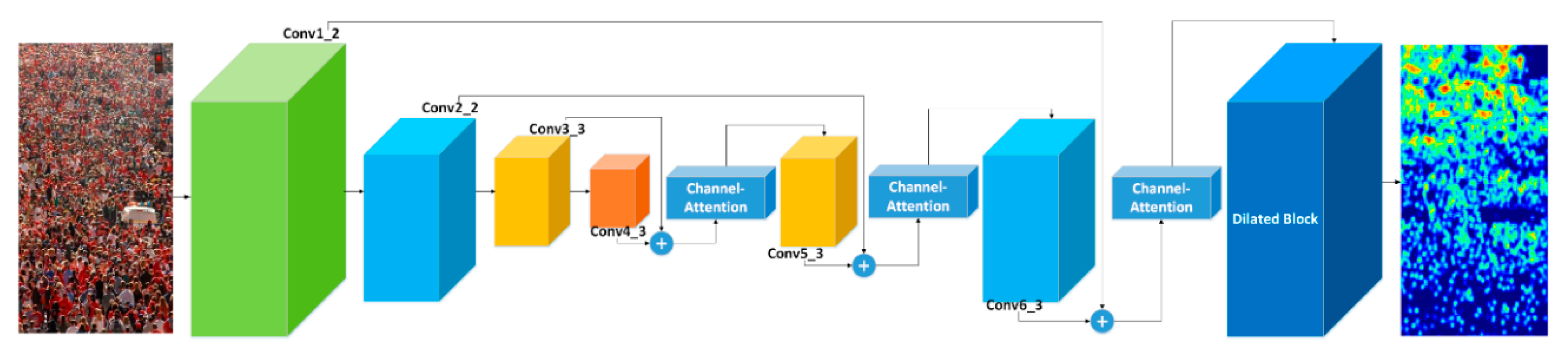
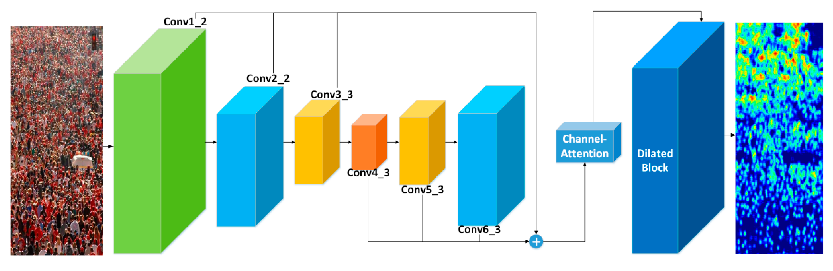
• We fuse the feature maps of the frontend and the backend. It has only a single column with convolutional kernels of one size, subtracting additional branches and multi-columns and reducing parameters. The convolutional layers of different levels contain not only different semantic information but also different scale feature information. Their fusion can deal with the large scale variation due to the perspective effect and the background interference, and share more features. It also requires fewer parameters and computation.
• We introduce the channel-attention block motived by Reference [10]. Avoiding the crude concatenate, the channel-attention block could take the weights of channels into consideration and ensure consummate fusion by enhancing the various scale features. On the other hand, it can conduct feature recalibration to capture spatial correlations and selectively emphasize informative features, so as to make the density map present a smooth transition between nearest pixels and improve the representation of our network.
• We utilize the dilated layer as the dilated block to the tail end of the network, which has less parameters but expands the receptive field. Furthermore, it contains more detailed global and spatial information to generate a high-quality density map.
• We subjoin SSIM to the loss function, which measures the local pattern consistency of the estimated density map and ground truth. So the final loss function has better representation of the difference between the estimation and the ground truth. Owing to it the accuracy can be greatly improved.

2. Related Work

Counting people in images and videos has attached attention in computer vision for a long time. Because it plays a significant role in video surveillance and public security. But the improvement of the estimation accuracy is quite a challenge on account of occlusions, perspective distortions, scale variations, and background interference. Up to now the research of crowd counting can be roughly summed up as the following three categories.

2.1. Detection-Based Methods

Early works detected the individuals and added them up to count. In 2012, Piotr Dollar et al. [17] used a moving-window-like detector to detect people and count the number in images. Haar wavelets classifier [18] was used to extract low-level features from the detected human body while Navneet Dalal et al. [19] replace it with HOG (histogram oriented gradients) classifier. Pedro F Felzenszwalb et al. [20] tried to detect some typical part of the body rather than the whole, because in crowd scenes human bodies were always occluded. But all these early works got awful results in congested scenes.

2.2. Regression-Based Methods

As scenes become more thronged, there is a limitation for detection-based methods to improve accuracy. So the regression-based methods were proposed. Antoni B Chan et al. [21] firstly used the foreground and texture features to generate low-level information, and the number of the crowd was calculated after learning the relations that the crowd corresponded to the extracted features. Then in 2013, Idrees et al. [2] introduced Fourier analysis and SIFT (Scale invariant feature transform) to extract features like [21]. But the saliency feature was easily overlooked, resulting in larger deviations. Then in [22], a linear mapping between features in the local region and its density maps was learned to integrate the information of saliency. In 2015, Pham et al. [23] proposed to learn a non-linear mapping instead of the linear one by random forest regression on account of the trouble in ideal linear mapping gain.

2.3. CNN-Based Methods

With the rapid development of the convolutional neural network, the brilliance in computer vision involved crowd counting was shown.

In 2015, Zhang et al. [24] trained CNNs to regress the crowd density map. They retrieved images using density and perspective information, then used them to fine-tune the trained network and predicted the density map. However, its applicability was limited by requirements of perspective maps and the fine-tuning of each test scene. In 2016, a multi-scale CNN architecture was used by Zhang et al. [16] to tackle the large scale variations in crowd scenes. And fully-connected layers were used to fuse the maps from each of the CNN trained at a particular scale to regress the density map. It aimed to solve the trouble in scale variation. Then, the multi-column [8,25] or multi-scale [3,7,12] network architecture was often utilized for crowd density regression. To be specific, Sam et al. [8] introduced a classifier to choose a specified column for training according to dense levels. Cao et al. [7] used a scale aggregation module as an encoder to extract features in diverse scales, and a group of transposed convolutions as a decoder to generate high-quality density maps. The local pattern consistency loss was as well proposed. Zhang et al. [12] combined the feature maps of multiple layers to adapt the changes in pedestrian scale and perspective and introduced a multi-task loss by adding a relative head count loss. But some works [11,12,13] suggested to replace diverse convolutional kernels with piles of the same size kernels. Li et al. [11] verified that the effectiveness of using multi-columns may not be prominent and that each column in such a branch structure had learned nearly identical features. They used VGG16 as the baseline and introduced dilated layers to the backend, which was a great improvement.

Furthermore, extra information was added to the training process to remedy background interference [14,15]. Shi et al. [14] proposed a self-supervised task to optimize the training of networks for crowd counting, leveraging unlabeled crowd images at training time to significantly improve performance. This generated a ranking of sub-images which were used to train a network to estimate whether one image contained more persons than another. Liu et al. [15] integrated the perspective information into crowd density maps for efficient crowd counting to provide additional information about the person scale change in an image. It was particularly helpful on the density regression of a small person area. However, extra information and tasks may require more resources and computations.

In 2019, more solutions have been proposed to solve this problem. Qi Wang et al. [26] constructed a large-scale and diverse synthetic crowd counting dataset to pretrain their designed Spatial Fully Convolutional Network. Weizhe Liu et al. [27] introduced an end-to-end architecture that combined features obtained using multiple receptive field sizes and learned the importance of each such feature at each image location. Chenchen Liu et al. [28] detected ambiguous image regions to zoom into high resolution for re-inspection, and added the localization task. Almost all the methods added extra information or tasks for enhancing the single counting task.

3. Our Proposed Method—FDCNet

Many previous methods introduced the multi-column fusion network architecture to reduce the errors caused from head scale variation due to the perspective effect. They can fuse the feature maps of various receptive fields from layers of various filter sizes or different columns. But various kernels may bring about more parameters and computations while multi-column architecture may make the network more complex. Hence, inspired by Reference [12], we propose to fuse the frontend and the backend feature maps of the one-column and one-size kernel network through channel-attention mechanism. The network will be more robust for the head scale variation and background noise, and meanwhile keep the conciseness. Furthermore, the dilated layer is exploited in the last part of our network, and SSIM-based loss is added into the loss function.

Our proposed architecture is shown in Figure 1. We call it FDCNet (Frontend-backend fusion dilated network through channel-attention mechanism). Next, we will elaborate on our model from four aspects.

3.1. The Frontend-Backend Fusion

During the collection of crowd scenes, the distance between pedestrians and cameras are not uniform. The head sizes would be different caused by the perspective effect, namely scale variety. In order to solve this problem and extract various scale features, we propose to fuse the frontend and backend feature maps in the crowd counting problem.

The backbone of our network is VGG-16. It has strong feature represent ability and easily to be concatenated. And we adopt the first 13 layers from VGG-16 to extract multi-scale feature maps. It composes with all the filter sizes as 3 × 3, the stacking several of which has the same effect as large filters. For example, the effect of two 3 × 3 filters cascade is the same as the 5 × 5 filter, and three 3 × 3 filters cascade could replace the 7 × 7 filter. Hence, it can extract various scale features but requires far less computation, and can build a deeper network.

The layers of different levels in the network contain not only the different level semantics information but also the different scale feature information. The frontend layers can extract the detail edge patterns, which are of significance for regressing the value of the congested region in the density map. But it cannot catch the details, which may cause incorrect regression with the cluttered backgrounds interference. The backend layers selectively obtain useful semantics information, so the network can distinguish the human heads from the background noise. In view of their specialties we fuse the frontend and the backend feature maps through the channel-attention block to acquire and fuse sufficient features from the backbone.

We use feature maps from Conv1_2, Conv2_2, Conv3_3, Conv4_3, and Conv5_3 in VGG backbone as shown in Figure 1 (Convi_j is the output feature map of the i_j layer in VGG-16 backbone). These inputs at different abstract levels help represent multi-scale features. Through the max pooling layers, the sizes of output feature maps are 1/2, 1/4, 1/8, and 1/16 of the original input images size, respectively.

First, the output of Conv4_3 is upsampled using nearest neighbor interpolation and is concatenated (put the two feature maps together in the first dimension) with Conv3_3. Then the fusion map is fed into the channel-attention block to adjust the weight of two layers fusion with different feature information and improve the representation of our network. Secondly, Conv5_3 and Conv2_2 are conducted like Conv4_3 and Conv3_3. Then, the output is also fed into the channel-attention block, followed by a group convolutional layers: conv1 × 1 × 512, conv3 × 3 × 512 and conv3 × 3 × 512. The 1 × 1 convolution before the 3 × 3 is used to reduce the computational complexity. After this procedure the output Conv6_3 is upsampled, concatenated with Conv1_2, and then is fed into the channel-attention block in the same way. Finally, the output feature map generates a density map after the process of the dilated block.

The channel-attention block and the dilated block are shown in Figure 2. We will introduce them specifically then.

3.2. The Channel-Attention Block

Attention Model has now become an important concept in neural networks that has been researched in diverse application domains [29]. Reference [10] introduced the SE building block. It models the interdependencies between the channels of its convolutional features so as to improve the representational power of a network.

Since most of the previous works directly combine the feature maps from different convolutions, they do not consider their respective weights when fusing. On the other hand, the channels of convolutional layers are always ignored, causing the deficiency of spatial information. The SE blocks can conduct the feature recalibration, selectively emphasizing informative features and suppressing less useful ones. Owing to that, the network can learn to use global information. Furthermore, it is also helpful for capturing spatial correlations without requiring additional supervision. One final point, it is computationally lightweight. With so many benefits, it only imposes a slight increase in model complexity and computational burden.

According to Reference [10], the SE block has been demonstrated to be accumulated through the entire network to improve the performance. Therefore, we transform the SE block to our framework as the channel-attention block. The specific architecture is shown in Figure 2a. The channel-attention block includes three processes: squeezing $S$, excitation $E$, and rescaling $R$.

The output feature map of the concatenation $N$ is firstly sent to a squeezing operation $S$. The squeezing operation aggregates the feature maps across the spatial dimension and generates channel-wise statistics through the global average pooling. The spatial dimension is $h\times w\times c$, which becomes $1\times 1\times c$ after shrinking. The corresponding channel descriptor $D_x\left(x=1,2,\cdots ,c\right)$ of the feature map in $N_x\left(x=1,2,\cdots ,c\right)$ each channel is calculated by:

$$D_x=S\left(N_x\right)=\frac{1}{h\times w}{{\displaystyle \sum }}_{i=1}^h{{\displaystyle \sum }}_{j=1}^w{n}_x\left(i,j\right)$$

(1)

where $n_x\left(i,j\right)$ is the element value of the $i$th row and the $j$th column on the feature map $N_x$. Through this we get the channel descriptor $D=\left\{D_x,x=1,2,\cdots ,c\right\}$. The channel descriptor embeds the global distribution of channel-wise feature responses, so that its lower layers are able to utilize the information of the global receptive fields.

Then, $D$ is fed into an excitation operation $E$, generating the extractor $T$. $E$ composes with two fully connected layers around the non-linearity, a Relu function and a sigmoid function. It is represented as:

$$T=E\left(D;FC\right)=\mathsf{\sigma }\left(g\left(D;FC\right)\right)=\mathsf{\sigma }({FC}_2\delta \left(F{C}_{1}D\right)$$

(2)

where $F{C}_1$ is a dimensionality-reduction layer with reduction ratio $k$, $k$ is a crucial hyperparameter which could vary the capacity and computational cost of the blocks in the model, and ${FC}_2$ is a dimensionality-increasing layer.

Following [10], we set $k=16$ to achieve a good balance between accuracy and complexity. $\delta$ is the Relu function, $\mathsf{\sigma }$ is the sigmoid function. The two fully connected layers can limit the model complexity by reducing the dimension and learning a nonlinear interaction between channels to fit the complex dependency of channels and aid generalization. Furthermore, the sigmoid activation emphasis multiple channels opposed to one-hot activation. The whole excitation operation fully captures channel-wise dependencies and governs the excitation of each channel, obtaining the normalized weights between 0 and 1.

Finally, the input of the channel-attention block $N$ is reweighted by the extractor $T$:

$$F=R\left(N;T\right)=T·N$$

(3)

where $R$ represents the channel-wise multiplication between the input feature map $N$ and the extractor $T$. That is, the weight of $T$ in each channel is weighted to each feature of the corresponding channel feature map in $N$ by means of multiplication, to complete the recalibration of the original feature on the channel dimension. The final output $F$ of the block can be fed directly into the next layers.

3.3. The Dilated Block

In our network, the input image of crowd is downsampled by the max pooling layers and upsamled before fusion. After those processes, the generated feature map is only half of the original input. The max pooling layers control overfitting and maintain invariance. Unfortunately, they reduce the spatial resolution so the spatial information of the feature map is lost. After passing through the max pooling layers, the feature maps are in lower resolution, and have difficulty in producing high-quality density maps.

In Reference [11], the dilated convolution is proved to maintain the resolution of the feature map better than the scheme of using the convolutional layer, pooling layer, and deconvolutional layer. Although deconvolutional layers can alleviate the loss of information, it would increase additional complexity and execution latency. Dilated convolution is a better choice to alternate the pooling layer. Based on this, we exploited the dilated convolutional layer in the tail end of our framework. The dilated convolution enlarges the receptive field without increasing the parameters or the computation amounts. Meanwhile, the output from dilated layers includes more detailed spatial and global information, and the spatial resolution would not be reduced. Hence, we could get a high-quality density map through the dilated convolutions and improve the estimation accuracy.

We tried a dilated convolution with a dilation rate of 2 in the tail end of our network. The dilated block is represented in Figure 2b. It composes four dilated layers with the dilation rate 2 and a convolutional layer of 1 × 1. The channels of dilated layers are all different and they are all followed by a batch normalization layer and a Relu layer. The 1 × 1 convolutional layer is to output the density map with fewer parameters and computation compared with the fully connected layer. The output from the dilated block can contain more detailed information. Finally we can retrieve the final density map of a high resolution.

3.4. The Loss Function

Mainstream works set pixel-wise Euclidean loss as their loss function in the training procedure. In the crowd scenes, the local patterns and texture features of the high-density regions vastly differ from other regions (low-density regions or background). However, the Euclidean loss is established on the pixel independence hypothesis and ignores them. The local correlation of density maps is not taken into consideration.

To remedy the aforementioned problems, we combined the loss function based on Structural Similarity Index (SSIM) with the Euclidean loss as our final loss function. The SSIM can be used to estimate the local consistency, optimizing the final loss function to measure the difference between the estimation and the ground truth. Owing to the training accuracy, the generation of high-quality density maps was improved.

3.4.1. The Euclidean Loss Function

The Euclidean loss function is used to measure the difference between the output and the corresponding ground truth at pixel level. The definition is as follows:

$$L_E\left(\mathsf{\Theta }\right)=\frac{1}{N}{{\displaystyle \sum }}_{i=1}^N{\left|\left|F_d\left(I_i;\mathsf{\Theta }\right)-D_i\right|\right|}^2$$

(4)

where $\mathsf{\Theta }$ denotes a set of the network parameters, and $N$ is the number of training samples. $F_d\left(I_i;\mathsf{\Theta }\right)$ represents the output estimated density map of the input image $I_i$ with parameters $\mathsf{\Theta }$, while $D_i$ is the corresponding ground truth density map.

3.4.2. The SSIM-Based Loss Function

SSIM is an indicator widely used in the field of image quality assessment. It computes the similarity between two images in terms of local patterns including mean, variance, and covariance. The range of SSIM value is from −1 to 1. The more similar two images are, the larger the value is. When the two images are identical, it is equal to 1.

We add SSIM to the loss function following SANet [7]. First, an 11 × 11 normalized Gaussian kernel with standard deviation of 1.5 is used to estimate local statistics. Then, the weight is defined by:

$$W=\left\{W\left(r\right)\right|r\in R,R=\left\{\left(-5,5\right),\cdots ,\left(-5,5\right)\right\}\}$$

(5)

where $r$ is offset from the center and $R$ contains all positions of the kernel. So for each location $t$, we calculate the local statistics on the estimated density map $F_d$ and the corresponding ground truth $D$.

First, the local mean ${\mu }_{F_d}$ and the variance estimation ${\sigma }_{F_d}^2$ of $F_d$ are respectively calculated by:

$${\mu }_{F_d}\left(t_{F_d}\right)={{\displaystyle \sum }}_{r_{F_d}ϵR_{F_d}}W\left(r_{F_d}\right)·F\left(t_{F_d}+r_{F_d}\right)$$

(6)

$${\sigma }_{F_d}^2\left(t_{F_d}\right)={{\displaystyle \sum }}_{r_{F_d}ϵR_{F_d}}W\left(r_{F_d}\right)·{\left[F\left(t_{F_d}+r_{F_d}\right)-{\mu }_{F_d}\left(t_{F_d}\right)\right]}^2$$

(7)

Then the local mean ${\mu }_D$ and the variance estimation ${\sigma }_D^2$ of $D$ are represented as:

$${\mu }_D\left(t_D\right)={{\displaystyle \sum }}_{r_DϵR_D}W\left(r_D\right)·F\left(t_D+r_D\right)$$

(8)

$${\sigma }_D^2\left(t_D\right)={{\displaystyle \sum }}_{r_DϵR_D}W\left(r_D\right)·{\left[F\left(t_D+r_D\right)-{\mu }_D\left(t_D\right)\right]}^2$$

(9)

Thereout the local covariance estimation ${\sigma }_{F_{d}D}$ between $F_d$ and $D$ is calculated by:

$${\sigma }_{F_{d}D}\left(t\right)={{\displaystyle \sum }}_{rϵR}W\left(r\right)·\left[F\left(t+r\right)-{\mu }_{F_d}\left(t_{F_d}\right)\right]·\left[Y\left(t+r\right)-{\mu }_D\left(t_D\right)\right]$$

(10)

After calculating these indexes, the SSIM is calculated point by point as:

$$\mathrm{SSIM}\left(t\right)=\frac{\left(2{\mu }_{F_d}{\mu }_D+Q_1\right)\left(2{\sigma }_{F_{d}D}+Q_2\right)}{\left({\mu }_{F_d}^2+{\mu }_D^2+Q_1\right)\left({\sigma }_{F_d}^2+{\sigma }_D^2+Q_2\right)}$$

(11)

$Q_1$ and $Q_2$ are randomly small constants to avoid division by zero and we set them following [7]. The SSIM-based loss function is introduced as:

$$L_s=1-\frac{1}{M}{{\displaystyle \sum }}_{t=1}^M\mathrm{SSIM}\left(t\right)$$

(12)

where $M$ is the number of pixels in density maps.

3.4.3. The Fusion Loss Function

After the SSIM-based loss penalty is added to the training process, the ultimate fusion loss function is introduced function as follows:

$$L=L_E+\beta L_s$$

(13)

where $\beta$ is the SSIM-based weight loss to get a balance. We set $\beta =0.001$ after experimenting for verification as well.

4. Experiments

4.1. Training Details and Data Augmentation

Our experiment is trained on four pieces of TITAN Xp GPU. The framework is based on the Pytorch framework, and we use the Adam optimizer to optimize the parameters and set the original learning rate as 1 × 10⁻⁶ and momentum at 0.9. The parameters are randomly initialized by Gaussian distribution with mean zero and standard deviation of 0.01. We also used batch normalization layers after every convolution layer except for the output layers to improve the speed of training and effectively avoid the disappearance and explosion of the gradient. We trained 2000 epochs for each dataset.

Given a training set, we augmented it by randomly cropping nine patches from each image. Each patch is 1/4 size of the original image. All patches were used to train our FDCNet.

4.2. Ground Truth Generation

Nowadays, the datasets generally provide the original images, the total numbers of crowds, and the corresponding coordinates of each person. Following the method of generating density maps in [16], we used the geometry-adaptive kernels to tackle the highly congested scenes. The geometry-adaptive kernel is defined as:

$$F\left(x\right)={{\displaystyle \sum }}_{i=1}^N\delta \left(x-x_i\right)\times G_{{\sigma }_i}\left(x\right),{\sigma }_i=\beta \overline{d_i}$$

(14)

where $x$ is the position of a pixel in the image. For each annotation $x_i$ in the ground truth $\delta$, we used $d_i$ to indicate the average distance of $k$ nearest neighbors. To generate the density map, we convolved $\delta \left(x-x_i\right)$ with a Gaussian kernel with the standard deviation ${\sigma }_i$, In our experiment, we followed the configuration in [16] and set $\beta =0.3,k=3$. By blurring each head annotation using a normalized Gaussian kernel, we generated the ground truth considering the spatial distribution of all images from each dataset.

4.3. Evaluation Metric

Most of the existing works use two metrics to estimate the accuracy for crowd counting, the mean absolute error (MAE), and the mean squared error (MSE). MAE indicates the accuracy of the estimation while MSE reflects the robustness of the estimation. Small values of MAE and MSE indicate good performance. The definitions are as follows:

$$\mathrm{MAE}=\frac{1}{N}{{\displaystyle \sum }}_{i=1}^N\left|F_{d_i}-D_i\right|$$

(15)

$$\mathrm{MSE}=\sqrt{\frac{1}{N}{{\displaystyle \sum }}_{i=1}^N{\left|F_{d_i}-D_i\right|}^2}$$

(16)

where $N$ is the number of the test images, $D_i$ is the actual number of crowd in the $i$th image, and $F_{d_i}$ is the estimated number of crowd in the $i$th image.

4.4. Performance on Common Datasets

We experimented on four common crowd datasets with various density and environments. These datasets are introduced and compared in

Table 1. Different dataset statistics.

Dataset	Average Resolution	Total Images	Min Number	Max Number	Avg Number	Total Number
ShanghaiTech Part A	589 × 868	482	33	3139	501	241,677
ShanghaiTech Part B	768 × 1024	716	9	578	124	88,488
UCF_CC_50	2101 × 2888	50	94	4543	1280	63,974
UCSD	238 × 158	2000	11	46	25	49,885
Mall	640 × 480	2000	13	53	31	62,325

and the results are compared to state-of-the-art methods to demonstrate our performance.

Figure 3 shows some output density maps. The first column are the original images from five datasets. The outputs of our FDCNet are in the third column. We also generated density maps from the VGG-16 backbone in the second column to compare the effectiveness of the two networks. Obviously, the density maps of our method show their brilliance.

We can see from the output density maps that our model solves the problems mentioned before well. All of the images have the background interference. The first three images are congested and have different head sizes. Compared to the VGG-16 backbone, the density far from the camera is much higher in the density map of FDCNet, matching the ground truth better. The last two images are sparse, having obvious background interference. The density map of our network for the fourth image is more accurate than that of VGG-16.

4.4.1. The ShanghaiTech Dataset

The ShanghaiTech crowd counting dataset is a diverse and crowded dataset introduced by Reference [16]. It has two parts, Part A and Part B. Part A is collected from the Internet. We can see from the Table 1 that it is mostly congested while Part B is taken from busy streets in Shanghai and is comparatively less dense with crowd counts. For Part A, 300 images are used for training and the remaining 182 images for testing. Similarly, 400 images of Part B are for training and 316 for testing.

Table 2. The estimation errors on ShanghaiTech dataset.

Method	Part A		Part B
	MAE	MSE	MAE	MSE
MCNN [16]	110.2	173.2	26.4	41.3
SwitchCNN [8]	90.4	135.0	21.6	33.4
SaCNN [12]	86.8	139.2	16.2	25.8
CSRNet [11]	68.2	115.0	10.6	16.0
FDCNet	75.1	118.5	10.3	15.8

reports the performance of our model along with other methods. It can be seen that our method got good estimations in the Part A dataset, nearly close to the result of CSRNet [11]. Furthermore, in the Part B dataset our method estimates better than other existing methods. It reflects that our model works well in extremely dense crowd scenes. Additionally, it may reflect that more experiments are required on this large dataset to improve the accuracy.

4.4.2. The UCF_CC_50 Dataset

The UCF_CC_50 dataset proposed by Idrees et al. [2] includes 50 images with different perspective and resolutions. It is an extremely congested dataset. Due to its limited images and various crowd counts and scenes, it is an extraordinary challenging dataset training for estimation. Hence, we perform five-fold-cross validation following the standard setting in Reference [2], making the utmost of the few samples.

Result comparisons of MAE and MSE are listed in

Table 3. The estimation errors on UCF_CC_50 dataset.

Method	MAE	MSE
MCNN [16]	377.6	509.1
SwitchCNN [8]	318.1	439.2
SaCNN [12]	314.9	424.8
CSRNet [11]	266.1	397.5
FDCNet	246.8	322.2

. The errors of our model are the smallest among all the models both in MAE and MSE, which indicates our method outperforms all other methods for crowd counting on the UCF_CC_50 dataset. Compared to CSRNet [11], the MAE was improved by 7.25%, and MSE was improved by 18.9%, which demonstrates its excellence for extremely dense crowds.

4.4.3. The UCSD Dataset

The UCSD dataset [30] is taken from a stationary camera. Similar to Reference [30], we use frames 601–1400 as the training set and the rest of them as the testing set. The results in

Table 4. The estimation errors on UCSD dataset.

Method	MAE	MSE
MCNN [16]	1.07	1.35
SwitchCNN [8]	1.62	2.10
CSRNet [11]	1.16	1.47
FDCNet	1.25	1.45

show that FDCNet gets better results than other methods in MSE. However, the result of MAE is a little worse than CSRNet [11], reflecting that our network does not do very well in the UCSD dataset. Seen from Figure 3, this dataset is a sparse dataset, which may get relatively lager errors when generating density maps due to the large intervals between heads. We therefore consider the need to experiment more on sparse datasets for better generalization.

4.4.4. The Mall Dataset

The Mall dataset [31] is collected in a shopping mall. We set the first 800 frames as the training dataset and the rest 1200 frames for testing following the pre-defined setting. Since it is not an extensive dataset in crowd counting, we compare our model with some approaches that did experiments in this dataset. The evaluation results are exhibited in

Table 5. The estimation errors on Mall dataset.

Method	MAE	MSE
R-FCN [32]	6.02	5.46
Exemplary Density [33]	1.82	2.74
FDCNet	1.80	2.52

. Our model performs the best compared to other models. Figure 3 shows that the mall dataset is also a sparse dataset, verifying that our network is also suitable for sparse datasets.

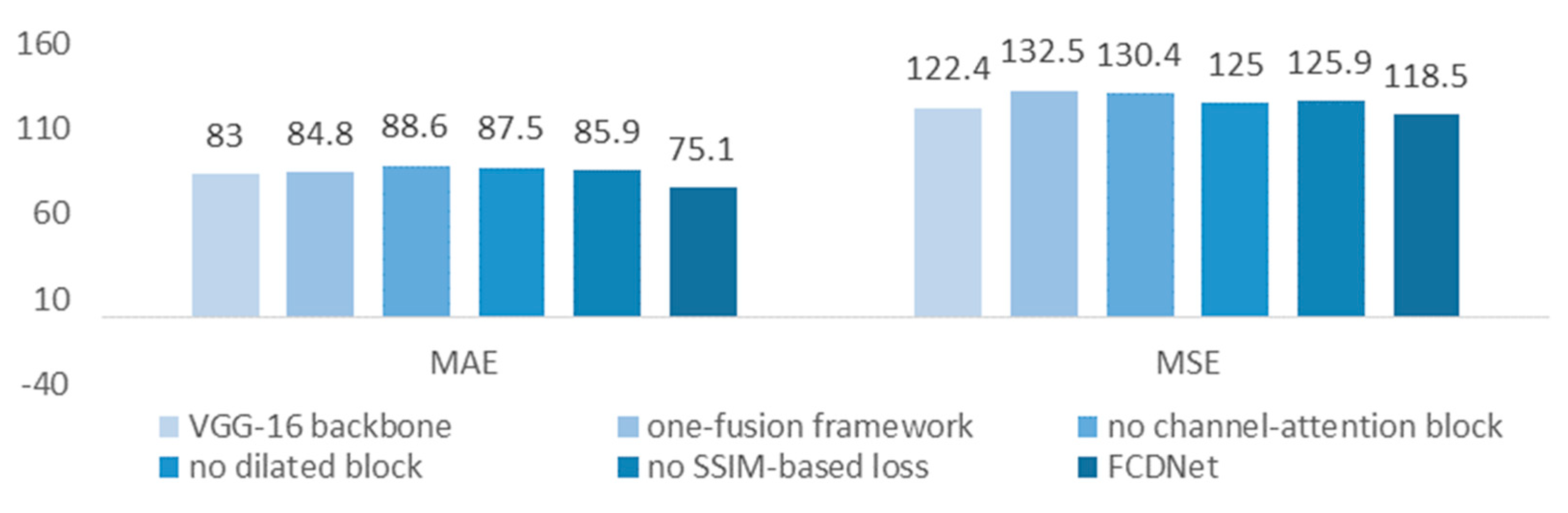
4.4.5. Ablation Study

We perform the ablation study to validate the efficacy of our FDCNet. Several ablation experiments are conducted on ShanghaiTech Part A dataset. The comparisons are shown in Figure 4, where the proposed framework gets the best estimation.

• VGG-16 framework

To verify the effectiveness of our method, we first did experiments on the backbone VGG-16 framework. The result in Figure 4 shows that our proposed framework improved the estimation more than the VGG-16, which implies that the improvements of our network are efficient and feasible.

Figure 3 demonstrates the output density maps from VGG-16 framework. Compared with the backbone results, we can see that our framework remedied the background interference and the perspective problem because the density maps are accurate in locating the head and eliminating the background. Furthermore, it is more suitable for congested images than VGG-16, as seen in the three extremely dense images.

• One-fusion framework

We have another choice to fuse different levels of feature maps before the dilated block, this is shown in Figure 5. The convolutional layers are set as FDCNet. There is only one fusion that Conv1_2, Conv2_2, Conv3_3, Conv4_3, Conv5_3, and Conv6_3 are concatenated together in the framework. After fusion the feature map is fed into the channel-attention block.

We trained using the ShanghaiTech Part A dataset on this one-fusion framework and compared the estimation with FDCNet. Seeing the results in Figure 4, the errors of one-fusion are much worse than FDCNet. It is obvious that FDCNet shows a more brilliant performance than the one-fusion framework.

On the one hand, the fusion of two levels can capture more varied scale features and send them to the next convolution, so that the backbone can extract more information. On the other hand, more channel-attention blocks following the fusion adjust them and obtain more spatial information. Owing to these factors, the FDCNet performs much better.

• The channel-attention block

We removed the three channel-attention blocks and let the output of the concatenation feed directly into the next convolutional layers. We can see from Figure 4 that the accuracy without channel-attention blocks are lower, which proves that the channel-attention block brings an awesome improvement with a slight computation.

• The dilated block

We do the experiments on our model to inspect the effect of using the dilated convolution. In the ablation study, the dilated layers in the dilated block are all replaced with the normal convolutional layers.

Figure 4 shows that both the MAE and MSE are much worse than that of FDCNet, respectively reduced by 6.5% and 3.7%. The results reflect that dilated convolution works better than the normal convolution without increasing the number of parameters or the amount of computation.

• The loss function

We also do experiments using only the L₂ loss function. Figure 4 reflects that both of the MAE and MSE of the fusion loss function are better. It proves that the SSIM-based loss does work. Since the SSIM compares the consistency between the estimated density map and the corresponding ground truth, the fusion loss function performs better than the merely L₂ loss.

5. Conclusions

This paper sets out to improve the accuracy of crowd counting. We proposed a FDCNet framework which is based on a single column network with a one size convolutional kernel but showed a brilliant performance. We introduced the fusion of the frontend features and the backend features, followed by the channel-attention blocks. The final feature maps are fed into the dilated block to produce density maps of high resolution. The estimations on four datasets perform well, some of which are better than the state-of-the-art versions. Our FDCNet is accurate, robust, and concise with a good generalization ability.

References

1. Idrees, H.; Soomro, K.; Shah, M. Detecting humans in dense crowds using locally-consistent scale prior and global occlusion reasoning. IEEE Trans. Pattern Anal. Mach. Intell. 2015, 37, 1986–1998. [Google Scholar] [CrossRef] [PubMed]
2. Idrees, H.; Saleemi, I.; Seibert, C.; Shah, M. Multi-source multi-scale counting in extremely dense crowd images. In Proceedings of the IEEE Conference on Computer Vision and Pattern Recognition, Portland, OR, USA, 25–27 June 2013; pp. 2547–2554. [Google Scholar]
3. Yang, J.; Zhou, Y.; Kung, S.Y. Multi-scale generative adversarial networks for crowd counting. In Proceedings of the IEEE International Conference on Pattern Recognition, Beijing, China, 20–24 August 2018; pp. 1051–4651. [Google Scholar]
4. Olmschenk, G.; Tang, H.; Zhu, Z. Crowd counting with minimal data using generative adversarial networks for multiple target regression. In Proceedings of the IEEE Winter Conference on Applications of Computer Vision, Lake Tahoe, CA, USA, 12–15 March 2018. [Google Scholar]
5. Liu, L.; Wang, H.; Li, G.; Ouyang, W.; Lin, L. Counting using Deep Recurrent Spatial-Aware Network. In Proceedings of the International Joint Conference on Artificial Intelligence, Stockholm, Sweden, 13–19 July 2018. [Google Scholar]
6. Sindagi, V.A.; Patel, V.M. Generating high-quality crowd density maps using contextual pyramid cnns. In Proceedings of the IEEE International Conference on Computer Vision, Venice, Italy, 22–29 October 2017; pp. 1879–1888. [Google Scholar]
7. Cao, X.; Wang, Z.; Zhao, Y.; Su, F. Scale aggregation network for accurate and efficient crowd counting. In Proceedings of the European Conference on Computer Vision, Munich, Germany, 8–14 September 2018; pp. 734–750. [Google Scholar]
8. Sam, D.B.; Surya, S.; Babu, R.V. Switching convolutional neural network for crowd counting. In Proceedings of the IEEE Conference on Computer Vision and Pattern Recognition, Honolulu, HI, USA, 21–26 July 2017; Volume 1, p. 6. [Google Scholar]
9. Sindagi, V.A.; Patel, V.M. Cnn-based cascaded multitask learning of high-level prior and density estimation for crowd counting. In Proceedings of the IEEE International Conference on Advanced Video and Signal Based Surveillance, Lecce, Italy, 29 August–1 September 2017; pp. 1–6. [Google Scholar]
10. Hu, J.; Shen, L.; Sun, G. Squeeze-and-excitation networks. In Proceedings of the IEEE Conference on Computer Vision and Pattern Recognition, Salt Lake City, UT, USA, 18–22 June 2018. [Google Scholar]
11. Li, Y.; Zhang, X.; Chen, D. Csrnet: Dilated convolutional neural networks for understanding the highly congested scenes. In Proceedings of the IEEE Conference on Computer Vision and Pattern Recognition, Salt Lake City, UT, USA, 18–22 June 2018; pp. 1091–1100. [Google Scholar]
12. Zhang, L.; Shi, M.; Chen, Q. Crowd counting via scale-adaptive convolutional neural network. In Proceedings of the IEEE Winter Conference on Applications of Computer Vision, Lake Tahoe, CA, USA, 12–15 March 2018; pp. 1113–1121. [Google Scholar]
13. Idrees, H.; Tayyab, M.; Athrey, K.; Zhang, D.; Al-Maadeed, S.; Rajpoot, N.; Shah, M. Composition loss for counting, density map estimation and localization in dense crowds. In Proceedings of the European Conference on Computer Vision, Munich, Germany, 8–14 September 2018; Springer: Berlin/Heidelberg, Germany, 2018; pp. 544–559. [Google Scholar]
14. Liu, X.; van de Weijer, J.; Bagdanov, A.D. Leveraging unlabeled data for crowd counting by learning to rank. In Proceedings of the IEEE Conference on Computer Vision and Pattern Recognition, Salt Lake City, UT, USA, 18–22 June 2018. [Google Scholar]
15. Shi, M.; Yang, Z.; Xu, C.; Chen, Q. Perspective-Aware CNN for Crowd Counting. In Proceedings of the 21st IEEE International Conference on Electronics, Bucharest, Romania, 29–31 October 2018. [Google Scholar]
16. Zhang, Y.; Zhou, D.; Chen, S.; Gao, S.; Ma, Y. Single image crowd counting via multi-column convolutional neural network. In Proceedings of the IEEE Conference on Computer Vision and Pattern Recognition, Las Vegas, NV, USA, 27–30 June 2016; pp. 589–597. [Google Scholar]
17. Dollar, P.; Wojek, C.; Schiele, B.; Perona, P. Pedestrian detection: An evaluation of the state of the art. IEEE Trans. Pattern Anal. Mach. Intell. 2012, 34, 743–761. [Google Scholar] [CrossRef] [PubMed]
18. Viola, P.; Jones, M.J. Robust real-time face detection. Int. J. Comput. Vis. 2004, 57, 137–154. [Google Scholar] [CrossRef]
19. Dalal, N.; Triggs, B. Histograms of oriented gradients for human detection. In Proceedings of the Computer Vision and Pattern Recognition, San Diego, CA, USA, 20–26 June 2005; Volume 1, pp. 886–893. [Google Scholar]
20. Felzenszwalb, P.F.; Girshick, R.B.; McAllester, D.; Ramanan, D. Object detection with discriminatively trained part-based models. IEEE Trans. Pattern Anal. Mach. Intell. 2010, 32, 1627–1645. [Google Scholar] [CrossRef]
21. Chan, A.B.; Vasconcelos, N. Bayesian poisson regression for crowd counting. In Proceedings of the IEEE 12th International Conference, Kyoto, Japan, 27 September–4 October 2009; pp. 545–551. [Google Scholar]
22. Lempitsky, V.; Zisserman, A. Learning to count objects in images. In Advances in Neural Information Processing Systems; The MIT Press: Cambridge, MA, USA, 2010; pp. 1324–1332. [Google Scholar]
23. Pham, V.Q.; Kozakaya, T.; Yamaguchi, O.; Okada, R. Count forest: Co-voting uncertain number of targets using random forest for crowd density estimation. In Proceedings of the Computer Vision IEEE International Conference, Santiago, Chile, 7–13 December 2015; IEEE Computer Society: Washington, DC, USA, 2015; pp. 3253–3261. [Google Scholar]
24. Zhang, C.; Li, H.; Wang, X.; Yang, X. Cross-scene crowd counting via deep convolutional neural networks. In Proceedings of the IEEE Conference on Computer Vision and Pattern Recognition, Boston, MA, USA, 7–12 June 2015; pp. 833–841. [Google Scholar]
25. Boominathan, L.; Kruthiventi, S.S.; Babu, R.V. Crowdnet: A deep convolutional network for dense crowd counting. In Proceedings of the ACM on Multimedia Conference, Amsterdam, The Netherlands, 15–19 October 2016; pp. 640–644. [Google Scholar]
26. Wang, Q.; Gao, J.; Lin, W.; Yuan, Y. Learning from synthetic data for crowd counting in the wild. In Proceedings of the Computer Vision and Pattern Recognition, Long Beach, CA, USA, 15–21 June 2019. [Google Scholar]
27. Liu, W.; Salzmann, M.; Fua, P. Context-aware crowd counting. In Proceedings of the Computer Vision and Pattern Recognition, Long Beach, CA, USA, 15–21 June 2019. [Google Scholar]
28. Liu, C.; Weng, X.; Mu, Y. Recurrent attentive zooming for joint crowd counting and precise localization. In Proceedings of the Computer Vision and Pattern Recognition, Long Beach, CA, USA, 15–21 June 2019. [Google Scholar]
29. Chaudhari, S.; Polatkan, G.; Ramanath, R.; Mithal, V. An Attentive Survey of Attention Models. Available online: https://arxiv.org/abs/1904.02874 (accessed on 5 April 2019).
30. Chan, A.B.; Liang, Z.S.J.; Vasconcelos, N. Privacy preserving crowd monitoring: Counting people without people models or tracking. In Proceedings of the Computer Vision and Pattern Recognition, Anchorage, AK, USA, 23–28 June 2008; pp. 1–7. [Google Scholar]
31. Chen, K.; Loy, C.C.; Gong, S.; Xiang, T. Feature mining for localized crowd counting. In Proceedings of the British Machine Vision Conference, Surrey, UK, 3–7 September 2012. [Google Scholar]
32. Dai, J.; Li, Y.; He, K.; Sun, J. R-fcn: Object detection via region-based fully convolutional networks. In Proceedings of the Neural Information Processing Systems, Barcelona, Spain, 5–10 December 2016. [Google Scholar]
33. Wang, Y.; Zou, Y. Fast visual object counting via example-based density estimation. In Proceedings of the 2016 IEEE International Conference on Image Processing, Phoenix, AZ, USA, 25–28 September 2016. [Google Scholar]
Figure 1. The architecture of our FDCNet (frontend-backend fusion dilated network through channel-attention mechanism) model. The input of the network is the original crowd image, which is fed into different convolutional groups. Conv1_2 et al. represent the feature maps output from different levels. The feature maps from the low level and high level are concatenated, then they are sent to the channel-attention blocks. In the end, the feature maps are fed into the dilated blocks, followed the output density map.
Applsci 09 03466 g001
Figure 2. (a) The architecture of the channel-attention block. (b) The architecture of the dilated block. The parameters in the first line are the sizes of the convolutional kernels and the channels.
Applsci 09 03466 g002
Figure 3. Some output density map of our FDCNet and the VGG-16 backbone. The first row are the original images in dataset, and the second row are the estimation density maps of the VGG-16 backbone. The third row are the estimation density maps of FDCNet. The images are selected from all datasets. They are selected from (a) ShanghaiTech Part A dataset; (b) ShanghaiTech Part B dataset; (c) UCF_CC_50 dataset; (d) UCSD dataset; (e) the mall dataset.
Applsci 09 03466 g003
Figure 4. The estimation errors of the ablation study.
Applsci 09 03466 g004
Figure 5. The architecture of the one-fusion framework.
Applsci 09 03466 g005