Fatigue Assessment on Suspenders under Stochastic Wind and Traffic Loads Based on In-Situ Monitoring Data

Featured Application

The present study attempts to predict the fatigue life of the suspenders through the incorporation of in-situ monitoring data into the proposed analytical coupled traffic-bridge-wind platform. The new findings highlight the importance of both wind load and traffic load in predicting the time-dependent fatigue reliability of the suspenders of long-span suspension bridges during their life time. It also brings an in-depth insight into the stress response characteristics of both the long suspender and short suspender under individual wind load, individual traffic load, as well as combined wind and traffic loads. The proposed methodology in this paper could provide essential guidelines for decision-making regarding the maintenance and replacement of suspenders.

Abstract

As a critical component of a suspension bridge, the integrity of the suspenders plays a critical role in the serviceability and reliability of the bridge during its life time. Despite the wide recognition of the importance of the suspenders, very few studies have been devoted to the condition evaluation of suspenders in operation. The present study performs the fatigue assessment on the suspenders accounting for the stochastic wind and traffic loads using the in-situ monitoring data. To this end, a probabilistic numerical framework is proposed to predict the time-dependent fatigue reliability of the suspenders under stochastic wind and traffic loads during the bridge’s life time, based on the linear fatigue damage rule. As a demonstration, the proposed numerical framework is applied to a long-span suspension bridge located in a mountainous canyon. The results indicate that it is of paramount importance to consider both the wind and traffic load effects in the fatigue reliability evaluation of the suspenders. In addition, it was also found that among the suspenders under investigation, the short suspender at the bridge mid-span (S36) is more prone to the fatigue damage, while the long suspender at the end of the bridge girder (S2) is less prone to the fatigue damage. Finally, provided with a target reliability index of 3.0, the fatigue life of the suspenders S36 and S2, considering the life time wind and traffic load, is estimated as 53 years and 167 years, respectively. The present research could provide essential guidelines for the optimization of inspection and replacement in maintenance practices for suspenders.

1. Introduction

Owing to the excellent spanning capacity and graceful appearance, more and more suspension bridges have been constructed/designed in recent years, serving as critical links in transportation networks, in order to cross larger water bodies, straits, or canyons. As the crucial force transmission components in suspension bridges, the suspenders are designed to transmit the roadway weight and the forces from the operational loads mainly from the vehicular traffic and wind to the primary force members. As a result, suspenders are inevitably subjected to continuously repeated stress cycles induced by operational loads during their lifetime. Thus, significant fatigue damage could accumulate at the suspenders, deteriorating the service performance of suspenders, which makes the suspenders among the most vulnerable bridge parts. Several prevention strategies have been proposed to protect the suspenders from deterioration, e.g., implementing energy absorbing devices at the bridge bearings or at the suspenders, the use of anti-corrosion materials, performing regular maintenance, etc. [1,2,3,4,5]. Nevertheless, there have been numerous reports worldwide regarding the premature damage of cables and suspenders due to fatigue, corrosion, or their coupled effects only after a few years of operation, resulting in traffic interruption, maintenance costs, or even total structural failure [6,7,8]. For a suspension bridge, the design life is 100 years or more, whereas the design life of a suspender is usually much less in mainland China [9]. Nevertheless, the fatigue life of different suspenders could vary dramatically, attributing to many factors such as the changing environments, the length and arrangement of suspenders, etc. Accurate assessment of the fatigue life of suspenders is not only critical to secure the serviceability and functionality of bridges, but also important to provide guidance for decision-making regarding the maintenance and replacement of the suspenders.

In recognizing the importance of the integrity of suspenders, many researchers throughout the world have proposed various approaches to investigating the deterioration mechanism of the suspenders, which can be mainly categorized into three groups, as follows: Experimental approaches [7,10], numerical approaches [11,12], and the combination of the former two approaches [9]. Recently, owing to the advanced structural health monitoring technology, there is an increasing trend in utilizing the in-situ measurement data for the fatigue assessment of suspenders [13], which further improves the credibility and accuracy.

Although extensive research has been conducted to reveal the deterioration mechanism of suspenders, a few challenges still remain unresolved regarding the accurate performance evaluation of suspenders. One major challenge is that the fatigue damage accumulation is a stochastic process subjected to various aleatory (random) and epistemic (lack of knowledge) uncertainties associated with material properties, operational loads, prediction modes, etc. For instance, laboratory tests on a group of degraded cables indicated that the Young’s modulus and ultimate strain follow the normal distributions, while the yield and ultimate stresses follow the Weibull distribution [9]. A numerical study conducted by Liu et al. [14] showed that the stochastic traffic load and wind load pose significant effects on the fatigue life of the suspenders. Compared with deterministic approaches, a probabilistic-based approach is a good alternative to tackle the uncertainties. Recently, Liu et al. [12] proposed a probabilistic numerical procedure for performing fatigue analysis on short suspenders under stochastic vehicular load. Similarly, Deng et al. [15] also presented a probabilistic fatigue assessment approach for suspenders based on structural monitoring, where the stochastic traffic was simulated using the Monte Carlo method. It should be noted that the above analyses have one major limitation, i.e., the vehicles were simplified as vertical load and only one vehicle was considered during the analysis. Even if the traffic flow is considered, critical parameters in the traffic flow, e.g., the vehicle type, vehicle speed, gross vehicle weight, and vehicle lane occupancy ratio, were not or only partially considered. Such simplification ignores the coupling effects between the traffic flow and the bridge, which may have significant influence on the dynamic behavior of the suspender and the resultant fatigue performance [16]. Additionally, there has been limited literature specifically focused on the effects of wind loads and the fatigue performance of the suspender considering site-specific wind load and traffic load has not been quantitatively evaluated.

In the present study, a probabilistic fatigue framework is proposed to evaluate the fatigue performance of the suspenders under stochastic wind and traffic loads, through the integration of in-situ monitoring data and the linear fatigue damage rule. First, the fully coupled traffic-bridge-wind (TBW) simulation is introduced. Subsequently, the stochastic wind and traffic load conditions at the bridge site are introduced, in which the associated key parameters are presented in detail. Furthermore, a probabilistic numerical framework is established to predict the time-dependent fatigue reliability of the suspenders based on the linear fatigue damage rule. As a demonstration, the proposed numerical framework is applied to a long-span suspension bridge located in a mountainous canyon. The stress response characteristics of both the long suspender and the short suspender under individual wind load, individual traffic load, as well as combined wind and traffic loads are investigated thoroughly. Finally, the fatigue life of the suspenders is estimated using Monte-Carlo simulations.

2. Fully Coupled Traffic-Bridge-Wind (TBW) Simulation

A fully coupled traffic-bridge-wind simulation platform based on the finite-element (FE) method was developed, which systematically incorporates the complex dynamic interactions among the bridge structure, stochastic wind, and traffic flow. The proposed platform is introduced in detail as follows.

2.1. Cellular Automaton Based Traffic Flow Simulation

Since the cellular automation (CA) model was first proposed for microscopic-scale traffic flow simulations in 1992 [17], the CA model has been widely employed to simulate the instantaneous behavior of vehicles in a stochastic traffic flow. The CA model enables efficient microscopic traffic flow simulation in the sense that the time advances in discrete steps and the space is discretized into a series of identical cells, each of which is either empty or occupied with up to one vehicle at a time [18]. In a CA model, the discrete variables in each cell are updated according to the vehicle information in the adjacent cells, through obeying a set of predefined traffic rules regulating accelerating, decelerating, breaking, and lane changing. Due to the high flexibility in modifying traffic rules, as well as readily incorporating various traffic information such as traffic density, vehicle type, gross vehicle weight, etc., the CA model has been validated to be able to capture realistic traffic features in heterogeneous traffic flow [17,19]. The CA model is adopted in the present study for stochastic traffic flow simulation and more details about CA mode can be referred to in References [20,21].

2.2. Modelling of Long-Span Suspension Bridge

A long-span suspension bridge over a deep gorge was selected as a prototype bridge in the present study. The suspension bridge is composed of a steel truss girder, concrete pylons, cables, and suspenders, which is modeled as a 3D finite-element model in ANSYS 15.0. The detailed modeling process is presented in latter sections of this paper.

2.3. Modelling of Road Vehicles

By pertaining all the relevant information, the vehicles can be simplified as several rigid bodies, suspension systems, and tires connected by a series of springs and dampers [22,23]. The vehicle bodies and the tires are simulated as rigid bodies, whereas the elasticity and dissipation capacities of both the suspension system and the tires are idealized as springs and dampers, respectively. Taking a 3-axle six-wheel road vehicle, shown in Figure 1, as an example, the vehicle was simplified as a combination of 8 rigid bodies, 3 wheel-axle sets, and 24 sets of springs and dampers in vertical and lateral directions. In total, 19 degree-of-freedoms (DOFs) are assigned for the 3-axle vehicle, including 8 independent vertical, 8 lateral, and 3 rotational DOFs. The corresponding response vector of the 3-axle vehicle is given by the following:

$${\mathbf{d}}_v=\left\{\begin{array}{c}{Z}_{vr}^1, Y_{vr}^1, {\theta }_{vr}^1, {\beta }_{vr}^1, Z_{vr}^2, Y_{vr}^2, {\beta }_{vr}^2, Z_{aL}^1, Z_{aL}^2, Z_{aL}^3\\ Z_{aR}^1, Z_{aR}^2, Z_{aR}^3, Y_{aL}^1, Y_{aL}^2, Y_{aL}^3, Y_{aR}^1, Y_{aR}^2, Y_{aR}^3\end{array}\right\},$$

(1)

where $Z_{vr}^i$ and $Y_{vr}^i$= vehicle vertical and lateral displacements of ith (i = 1, 2) rigid body; ${\theta }_{vr}^i$ and ${\beta }_{vr}^i$= rotational displacements of ith (i = 1, 2) rigid body in the X-Z plane (pitching) and the Y-Z plane (rolling), respectively; $Z_{aL\left(R\right)}^j$ = vertical displacement of jth (j = 1, 2, 3) wheel axle on the left (right) side; $Y_{aL\left(R\right)}^j$ = lateral displacement of jth (j = 1, 2, 3) wheel axle on the left (right) side. Each DOF in the vector is independent, as shown in Figure 1a,b. The ${\theta }_{vr}^2$ is dependent on other DOFs, which is defined as ${\theta }_{vr}^2=\left(Z_{vr}^2-Z_{vr}^1-L_5 {\theta }_{vr}^1\right)/L_6$.

2.4. Modelling of Wind Forces on Bridge

The wind-induced forces on bridge girders are commonly decomposed into three components, as follows: Static wind forces due to mean wind speed, self-excited forces due to wind-bridge interactions, and buffeting forces due to wind turbulences [23,24,25]. Additionally, each wind component can be further discretized as lift force, drag force, and torsional moments. For the bridge pylons, main cables, and suspenders, only drag force from static wind speed is considered [2].

The self-excited forces can be calculated by summing the responses associated with the structural motion in lateral, vertical, and torsional directions. Specifically, the self-excited drag force, lift force, and torsional moments acting on bridge girder per unit length are derived as the convolution integrals between the arbitrary bridge girder motion and the associated impulse functions, as shown below [26]:

$$\begin{array}{c}{D}_{se}\left(t\right)=D_{sep}\left(t\right)+D_{seh}\left(t\right)+D_{se\alpha }\left(t\right)={{\displaystyle \int }}_{-\infty }^t(f_{Dp}\left(t-\tau \right)p\left(\tau \right)+f_{Dh}\left(t-\tau \right)h\left(\tau \right)+\\ f_{D\alpha }\left(t-\tau \right)\alpha \left(\tau \right))d\tau ,\end{array}$$

(2a)

$$\begin{array}{c}{L}_{se}\left(t\right)=L_{sep}\left(t\right)+L_{seh}\left(t\right)+L_{se\alpha }\left(t\right)={{\displaystyle \int }}_{-\infty }^t(f_{Lp}\left(t-\tau \right)p\left(\tau \right)+f_{Lh}\left(t-\tau \right)h\left(\tau \right)+\\ f_{L\alpha }\left(t-\tau \right)\alpha \left(\tau \right))d\tau ,\end{array}$$

(2b)

$$\begin{array}{c}{M}_{se}\left(t\right)=M_{sep}\left(t\right)+M_{seh}\left(t\right)+M_{se\alpha }\left(t\right)={{\displaystyle \int }}_{-\infty }^t(f_{Mp}\left(t-\tau \right)p\left(\tau \right)+f_{Mh}\left(t-\tau \right)h\left(\tau \right)+\\ f_{M\alpha }\left(t-\tau \right)\alpha \left(\tau \right))d\tau ,\end{array}$$

(2c)

where f = response impulse functions that are derived by experimentally determined flutter derivatives based on the rational approximation approach; the subscripts D, L, and M = response contribution to the self-excited drag force, lift force, and torsional moment; the subscripts p, h, and α = impulse response functions with respect to unit impulse displacements in the lateral, vertical, and torsional directions, respectively; and p(τ), h(τ), and α(τ) are the time-dependent lateral, vertical, and rotational displacements of the bridge girder. For each impulse response function, the corresponding frequency function can be represented by rational functions. The frequency independent parameters are obtained through least square fitting of flutter derivatives. Once the frequency response functions are computed, the impulse response functions are then derived using the Fourier transform for each motion.

The buffeting forces acting on the bridge girder are due to the unsteady wind turbulence on both horizontal and vertical directions. Similar to the way in which the self-excited forces are constructed, the buffeting forces on the bridge girder per unit span can be expressed as the convolution integral between the wind turbulence and associated impulse response functions, as follows:

$$D_b\left(t\right)=D_{bu}\left(t\right)+D_{bw}\left(t\right)={{\displaystyle \int }}_{-\infty }^t\left(f_{Du}\left(t-\tau \right)u\left(\tau \right)+f_{Dw}\left(t-\tau \right)w\left(\tau \right)\right)d\tau ,$$

(3a)

$$L_b\left(t\right)=L_{bu}\left(t\right)+L_{bw}\left(t\right)={{\displaystyle \int }}_{-\infty }^t\left(f_{Lu}\left(t-\tau \right)u\left(\tau \right)+f_{Lw}\left(t-\tau \right)w\left(\tau \right)\right)d\tau ,$$

(3b)

$$M_b\left(t\right)=M_{bu}\left(t\right)+M_{bw}\left(t\right)={{\displaystyle \int }}_{-\infty }^t\left(f_{Mu}\left(t-\tau \right)u\left(\tau \right)+f_{Mw}\left(t-\tau \right)w\left(\tau \right)\right)d\tau ,$$

(3c)

where u and w = turbulent wind in horizontal (normal to bridge longitudinal axis) and vertical direction; f_Du(t), f_Dw(t), f_Lu(t), f_Lw(t), f_Mu(t), and f_Mw(t) = the impulse response functions, where the subscripts D, L, and M = impulse response functions in terms of drag force, list force, and torsional moment and the subscripts u and w = the impulse response functions corresponding to wind turbulence in the horizontal and vertical directions. Similar to the way in which the self-excited forces are constructed, the buffeting forces are formulated using frequency dependent aerodynamic admittance functions.

It should be noted that both the flutter derivatives and the aerodynamic admittance functions are determined through the wind tunnel experiments. For more details, readers are referred to Reference [2].

2.5. Modelling of Wind Forces on Road Vehicles

The total wind force on running vehicles can be formulated based on quasi-static approach [27], as follow:

$$\{\begin{array}{c}{F}_S=0.5\rho U_r^2\left(t\right)C_S\left(\Psi \right)A_0; F_L=0.5\rho U_r^2\left(t\right)C_L\left(\Psi \right)A_0; F_D=0.5\rho U_r^2\left(t\right)C_D\left(\Psi \right)A_0;\\ M_P=0.5\rho U_r^2\left(t\right)C_P\left(\Psi \right)A_0{h}_v; M_Y=0.5\rho U_r^2\left(t\right)C_Y\left(\Psi \right)A_0{h}_v; M_R=0.5\rho U_r^2\left(t\right)C_R\left(\Psi \right)A_0{h}_v; \end{array},$$

(4)

where F_S, F_L, F_D, M_P, M_Y, and M_R = side force, lift force, drag force, pitching moment, yawing moment, and rolling moment on the vehicle, respectively; C_S(Ψ), C_L(Ψ), C_D(Ψ), C_P(Ψ), C_Y(Ψ), and C_R(Ψ) = wind aerodynamic coefficients with respect to six wind forces; A₀ = the reference area of the vehicle; h_v = the distance from the vehicle gravity center to the road surface; U_r is the relative wind velocity to the vehicle; and ψ = the yaw angle defined as the angle between the direction of relative wind speed and the vehicle driving direction. The U_r and Ψ are given by the following:

$$\{\begin{array}{c}{U}_r=\sqrt{{\left(U+u\left(x, t\right)\right)}^2+U_{ve}^2\left(t\right)}\\ \Psi =\arctan \left[U+u\left(x,t\right)/U_{ve}\left(t\right)\right]\end{array},$$

(5)

where U = the mean wind speed; u(x, t) = the horizontal wind turbulence at the x coordinate along the bridge axis at time step t; and U_ve = vehicle speed.

It is noted that the wind aerodynamic coefficients for the vehicles can be experimentally determined using the following equation:

$$\{\begin{array}{c}{C}_S=\frac{{\overline{F}}_s}{0.5\rho U^2{A}_0} C_L=\frac{{\overline{F}}_L}{0.5\rho U^2{A}_0}; C_D=\frac{{\overline{F}}_D}{0.5\rho U^2{A}_0};\\ C_P=\frac{{\overline{M}}_P}{0.5\rho U^2{A}_0{h}_v}; C_Y=\frac{{\overline{M}}_Y}{0.5\rho U^2{A}_0{h}_v}; C_R=\frac{{\overline{M}}_R}{0.5\rho U^2{A}_0{h}_v};\end{array},$$

(6)

where ${\overline{F}}_s$, ${\overline{F}}_L$, and ${\overline{F}}_D$ are the mean values of the aerodynamic side force, lift force, and drag force during the wind tunnel test and ${\overline{M}}_P$, ${\overline{M}}_Y$, and ${\overline{M}}_R$ are the mean values of the pitching moment, yawing moment, and rolling moment during the wind tunnel test.

2.6. Governing Equations of Motion for the TBW Coupled System

The governing equations of motions for the coupled traffic-bridge-wind system are given as follows below:

$$\begin{array}{c}\left[\begin{array}{cc}\begin{array}{cc}{M}_b& 0\\ 0& M_{v1}\end{array}& \begin{array}{cc}\cdots & 0\\ \cdots & 0\end{array}\\ \begin{array}{cc} ⋮& ⋮ \\ 0& 0\end{array}& \begin{array}{cc} \ddots & ⋮ \\ \cdots & M_{vn}\end{array}\end{array}\right]\left\{\begin{array}{c}{\ddot{q}}_b\\ {\ddot{q}}_{v1}\\ ⋮\\ {\ddot{q}}_{vn}\end{array}\right\}+\left[\begin{array}{cc}\begin{array}{cc}{C}_b& 0\\ 0& C_{v1}\end{array}& \begin{array}{cc}\cdots & 0\\ \cdots & 0\end{array}\\ \begin{array}{cc} ⋮& ⋮ \\ 0& 0\end{array}& \begin{array}{cc} \ddots & ⋮ \\ \cdots & C_{vn}\end{array}\end{array}\right]\left\{\begin{array}{c}{\dot{q}}_b\\ {\dot{q}}_{v1}\\ ⋮\\ {\dot{q}}_{vn}\end{array}\right\}\\ +\left[\begin{array}{cc}\begin{array}{cc}{K}_b& 0\\ 0& K_{v1}\end{array}& \begin{array}{cc}\cdots & 0\\ \cdots & 0\end{array}\\ \begin{array}{cc} ⋮& ⋮ \\ 0& 0\end{array}& \begin{array}{cc} \ddots & ⋮ \\ \cdots & K_{vn}\end{array}\end{array}\right]\left\{\begin{array}{c}{q}_b\\ q_{v1}\\ ⋮\\ q_{vn}\end{array}\right\}=\left\{\begin{array}{c}({{\displaystyle \sum }}_{i=1}^n{F}_{vi}^G)+F_b^R+F_b^C+F_b^{Se}+F_b^{Bu}\\ F_{v1}^R+F_{v1}^C+F_{v1}^W\\ ⋮\\ F_{vn}^R+F_{vn}^C+F_{vn}^W\end{array}\right\},\end{array}$$

(7)

where n = the total number of vehicles in the traffic flow; q = the displacement vector; M, F, C, and F = structural mass, stiffness, damping matrices, and force vector; subscripts b and v_i (i = 1,2,…n) indicate the parameters for bridge and ith vehicle, respectively; and the superscripts G, R, C, W, Se, and Bu = excitation loads from gravity, road surface roughness, coupling interaction forces, static wind, self-excited and buffering forces, respectively. The coupling interaction force between the bridge and the ith vehicle are given by:

$$\{\begin{array}{c}{F}_b^C={{\displaystyle \sum }}_{i=1}^n{C}_{bci}\left\{{\dot{q}}_b\right\}+{{\displaystyle \sum }}_{i=1}^n{K}_{bci}\left\{q_b\right\}+{{\displaystyle \sum }}_{i=1}^n{C}_{b, v_i}\left\{{\dot{q}}_{v_i}\right\}+{{\displaystyle \sum }}_{i=1}^n{K}_{b, v_i}\left\{q_{v_i}\right\}\\ F_{v_i}^C=C_{v_i,b}\left\{{\dot{q}}_{v_i}\right\}+K_{v_i,b}\left\{q_{v_i}\right\}\end{array},$$

(8)

where K_bci and C_bci = stiffness and damping contribution to the bridge caused by the coupling effects between bridge and ith vehicle in the traffic flow and $K_{b,v_i}$($K_{v_i,b}$) and $C_{b,v_i}$($C_{v_i,b}$) are the coupled stiffness and damping matrices between the bridge and the vibration of ith vehicle, respectively.

As the complicated dynamic coupling effects among the bridge, traffic, and wind cannot be modeled appropriately using the existing finite element (FE) software, an analytical framework of the coupled TBW dynamic system was established using the computer programming language MATLAB and commercial FE software ANSYS. The whole simulation process is composed of three steps. Firstly, the numerical models for the bridge and vehicles are established to obtain the initial coefficient matrices in ANSYS. Secondly, the stochastic wind field and traffic flow are simulated to calculate the wind forces on the bridge/vehicle as well as the coupled bridge-vehicle forces. Thirdly, the governing equations of the coupled TBW system are developed to perform the dynamic analysis in MATLAB. In this step, the geometric nonlinear effect of axial forces on the bridge girder and pylons and the cable tension can be taken into account. After the coupled governing equations are solved, the stress vector can be further computed based on the deflection-strain relationship and the stress-strain relationship, as given by the following:

$$\left[S\right]=\left[E\right]\left[B\right]\left\{q_b\right\},$$

(9)

where [S] = the predicted stress vector; [E] = the stress-strain relationship matrix, which is assumed to be constant; and [B] = the stress-deflection relationship matrix deduced from the element shape functions.

3. Stochastic Load Conditions

3.1. Wind Environments

The wind information at the bridge site is necessary for fatigue damage evaluation. The wind records of 10 min mean wind speed and direction from the anemometer installed on the bridge tower from the period between 1 March 2008 and 31 December 2010 are used in the present study for wind data analysis [25]. The wind velocities were collected from the anemometer, with a height of 150 m above the ground level, and were further transformed to the wind velocity at the bridge deck level via the wind profile power law with the exponent being 0.2. The wind records were carefully checked to exclude any abnormal records. All the wind records were classified into 16 sectors of the compass with an interval of Δθ = 22.5°, according to the wind directions. In each sector, the mean wind speed was further divided into 7 ranges from 0 to 21 m/s with an interval of ΔU = 3 m/s. As a result, a total of 112 cells were used, in which each cell recorded the relative frequency associated with the corresponding wind speed and wind direction, as tabulated in

Table 1. ¹ Relative frequency of mean wind speed and direction (%).

Wind Direction	0–3	3–6	6–9	9–12	12–15	15–18	18–21	Sum
N (0°)	0.688	2.103	2.574	0.476	0.284	0.000	0.000	6.125
NNE (22.5°)	1.220	3.514	5.694	1.326	0.424	0.240	0.005	12.423
NE (45°)	0.728	2.604	3.136	0.857	0.356	0.144	0.000	7.825
ENE (67.5°)	0.496	0.876	1.324	0.759	0.208	0.000	0.000	3.663
E (90°)	0.356	1.285	1.098	0.662	0.444	0.000	0.000	3.844
ESE (112.5°)	0.248	1.027	1.324	0.891	0.252	0.000	0.000	3.742
SE (135°)	0.416	0.851	1.024	1.021	0.356	0.000	0.000	3.668
SSE (157.5°)	3.496	2.604	0.752	0.775	0.314	0.096	0.000	8.037
S (180°)	0.840	3.347	2.724	1.326	0.216	0.096	0.000	8.549
SSW (202.5°)	0.916	4.624	6.563	1.376	0.483	0.360	0.005	14.327
SW (225°)	1.204	2.679	2.620	0.958	0.346	0.000	0.000	7.806
WSW (247.5°)	0.416	1.878	1.936	0.837	0.194	0.000	0.000	5.261
W (270°)	0.388	1.327	1.352	0.705	0.420	0.000	0.000	4.192
WNW (292.5°)	0.296	1.895	0.612	0.583	0.225	0.000	0.000	3.610
NW (315°)	0.208	1.436	0.483	0.485	0.264	0.072	0.000	2.947
NNW (337.5°)	0.452	1.269	1.575	0.416	0.208	0.060	0.000	3.980
Sum	12.368	33.317	34.791	13.451	4.994	1.068	0.010	100.0

¹ The mean wind velocity refers to the 10 min mean wind at the bridge deck level and the unit of wind velocity is m/s.

. In Table 1, the last row displays the relative frequency of mean wind speed without considering the wind direction, while the last column lists the relative frequency of wind direction without considering the wind speed. For better illustration, the wind data are also displayed as the wind rose map, as shown in Figure 2. The bridge alignment, normal to the gorge axis and directed from the ESE (112.5°) to WNW (292.5°), is also depicted in Figure 2 for reference. It is observed from Figure 2b that the prevailing wind blows from NNE or SSW, i.e., along the axis of the gorge and normal to the bridge alignment. It is also shown in Figure 2a that the prevailing wind has a relatively larger wind speed compared with the wind in other directions.

The relative angle between the wind direction and the bridge alignment has a significant influence on the resultant bridge dynamic response. Many researchers have reported that the wind with the direction normal to the bridge alignment (i.e., cross-wind) could induce the largest bridge dynamic responses, while the wind with direction parallel to the bridge axis could barely affect the bridge dynamic responses [28]. Therefore, it is assumed that the contribution of cross-wind to fatigue damage accumulation is much more significant than that caused by the wind parallel to the bridge alignment [2]. To this end, in the present study, all the winds were decomposed into two components, one normal to the bridge axis and one parallel to the bridge axis, and only the cross-wind was adopted for the subsequent analysis. As a result, the cross-winds at the bridge site were obtained and eight cross-winds were chosen to represent the cross-wind ranges in the bridge location with the probability occurrence, as tabulated in

Table 2. Representative mean cross-wind and probability of occurrence.

Number	U	Range (m/s)	Probability of Occurrence (%)
1	0 (no wind)	<0.5	24.837
2	2.0 m/s	0.5–3	9.293
3	4.5 m/s	3–6	24.614
4	7.5 m/s	6–9	27.935
5	10.5 m/s	9–12	9.113
6	13.5 m/s	12–15	3.239
7	16.5 m/s	15–18	0.960
8	20.0 m/s	>18	0.010

.

3.2. Traffic Conditions

It is noteworthy that the traffic condition plays a significant role in evaluating the fatigue damage accumulation of the suspenders. A video containing 48 consecutive hours of traffic data on the suspension bridge was analyzed to obtain the essential traffic information, including the vehicle type, gross vehicle weight (GVW), lane occupancy, traffic density, etc. According to the traffic data, the vehicles could be categorized into seven types denoted as V1–V7, where V1 represents 2-axle mini-vans, V2 represents 2-axle sedan cars, and V3–V7 represent 2- to 7-axle trucks. The suspension bridge supports two-way four traffic lanes, and the hourly traffic volume (denoted as η for abbreviation) for the fast lane and the slow lane is illustrated in Figure 3a,b, respectively. Figure 3a,b show that the hourly traffic volume for both lanes is time-dependent and has the similar pattern; η is lower and relatively stable during 0:00–10:00 and 20:00–24:00, while η is much higher and stable during 10:00–20:00. To this end, by setting the threshold value as 200 vehicles per hour, the traffic conditions at the bridge site fall into two categories, as follows: (1) Free-flow with about 110 vehicles and 90 vehicles per hour for the fast lane and the slow lane, respectively; and (2) busy-flow with about 360 vehicles and 300 vehicles per hour for the fast lane and the slow lane, respectively. The probability of occurrence of free-flow condition and busy-flow condition is 0.583 (i.e., 14 h in one day) and 0.417 (i.e., 10 h in one day), respectively. Additionally, further analysis revealed that the vehicle occupancy ratios at each lane remained stable during the entire time, thus the vehicle occupancy ratios listed in

Table 3. Vehicle categories and the corresponding traffic lane occupancy ratios (×100%).

Vehicle Type	Fast Lane		Slow Lane
	Number of Vehicles in 1 Day	Occupancy Ratio	Number of Vehicles in 1 Day	Occupancy Ratio
V1 (2-axle mini-van)	312	3.22	543	5.60
V2 (2-axle sedan car)	3326	34.28	463	4.77
V3 (2-axle truck)	305	3.14	635	6.55
V4 (3-axle truck)	346	3.57	680	7.01
V5 (4-axle truck)	402	4.14	643	6.63
V6 (5-axle truck)	383	3.95	702	7.24
V7 (6-axle truck)	321	3.30	642	6.62
Total	5395	55.60	4308	44.40

were employed for simulating both the free-flow traffic and busy-flow traffic conditions.

In addition to the traffic density and vehicle type, the vehicle gross vehicle weight (GVW) is also an important factor for traffic flow simulations. In the present study, the GVW of each vehicle type was first obtained and then fitted with commonly used distribution models. The suitability of the proposed distributions was examined by comparing their log-likelihood values and the distribution model with the maximum log-likelihood value was selected as a best fit [16]. It was found that the GVW of all the 7 types of vehicle followed the single-peak distribution and the optimal distribution model with the parameters for each type of vehicle is summarized in

Table 4. Probabilistic properties of GVW for each type of vehicle (kN).

Vehicle Type	Distribution Type	Mean Value (μ)	Standard Deviation (σ)
V1	Lognormal	16.46	4.82
V2	Lognormal	14.51	3.54
V3	Normal	35.72	9.72
V4	Normal	123.95	18.72
V5	Lognormal	69.74	10.28
V6	Normal	291.04	43.21
V7	Normal	528.32	85.21

.

With the vehicle information obtained through the analysis of the vehicle data, the traffic flow could be simulated based on the CA model. The simulation process mainly consists of three steps, which are briefly introduced herein:

(1)

Firstly, the number of vehicles for each vehicle type (V1–V7) was determined by multiplying the corresponding occupancy rate (in Table 3) with the effective daily traffic volume.

(2)

Secondly, for each vehicle type, Latin hypercube sampling was conducted to obtain samples of GVW through the established distribution model (in Table 4), which was further assigned to each individual vehicle of that vehicle type.

(3)

Thirdly, the traffic density and the information of each individual vehicle (with the vehicle type and GVW) were put into the CA model for stochastic traffic simulation.

As an illustration, Figure 4 displays the simulated traffic on the fast lane and slow lane under both free-flow and busy-flow traffic conditions. Each short line in Figure 4 represents one vehicle, and various colors are assigned to the short line to differentiate various vehicle categories. It is observed from Figure 4 that free-flow and busy-flow traffic exhibits different traffic patterns, i.e., the vehicles under free-flow traffic conditions (Figure 4a,c) drive smoothly without experiencing any traffic congestion, while the vehicles under busy-flow traffic conditions (Figure 4b,d) experience few times of traffic congestions. This is due to the fact that the traffic volume under busy-flow traffic condition is significantly higher than that under free-flow traffic conditions (refer to Figure 3), which could cause traffic congestions.

In order to further evaluate the performance of the proposed CA-based stochastic traffic flow model, the predicted distributions of the gross vehicle weight in the simulated traffic flow were compared with the corresponding target distributions (refer to Table 4), as shown in Figure 5. It is observed from Figure 5 that the predicted GVW distributions match quite well with the target distributions for V1, V3, V5, and V7 vehicles. It is worth mentioning that the predicted GVW distribution for V2, V4, and V6 also match quite well with the target distribution. Therefore, the simulated stochastic traffic flow can accurately reflect the site-specific traffic statistics.

4. Probabilistic Fatigue Reliability Assessment

4.1. S-N Approach and Miner’s Rule

The Miner’s linear fatigue damage accumulation theory together with the S-N curve (stress life) has been widely employed for structural fatigue damage assessment. Design codes such as AASHTO [29] and Eurocode 3 [30] have proposed a set of S-N curves, defined as the nominal stress range versus life in cycles, for fatigue assessment on various detail categories. In the present study, the AASHTO specification is used, in which the S-N curve is expressed as follows:

$$S={\left(A/N\right)}^{1/m},$$

(10)

where S = constant stress range, N = fatigue life of a detail, m = 3 is the slope of the S-N curves, and A = detail constant.

It is noteworthy that the fatigue stresses of the suspenders caused by the stochastic loads are random variables, whereas the S-N curve is originally applicable for constant-amplitude fatigue stresses. To this end, the Miner’s linear fatigue damage accumulation theory, termed as Miner’s rule, was proposed to account for the variable amplitude stresses [31]. The Miner’s rule simply assumes that the fatigue damage fraction at any particular stress range level is a linear function of the corresponding number of cycles, and therefore, the total fatigue damage accumulation can be expressed as the sum of damage caused by each individual stress range level.

$$D_a={{\displaystyle \sum }}_i\frac{n_i{S}_{ri}^m}{A},$$

(11)

where D_a = the fatigue damage accumulation and n_i = the number of cycles at stress range S_ri. The number of cycles n_i and stress range S_ri are obtained from the stress range bin histogram using the rain-flow counting method [31].

The fatigue damage accumulation D_a is typically equal to 1.0 at failure, while it may be less than 1.0 due to various uncertainties [32]. By applying the Miner’s rule, the equivalent fatigue stress range and corresponding number of cycles can be derived as follows:

$$S_{re}=\left({{\displaystyle \sum }}_i\frac{n_i}{n_t}·S_{ri}^m\right).$$

(12)

where S_re = the equivalent fatigue stress range and n_t = ∑_i(n_i) is the total number of stress cycles. It should be noted that the S_re and n_t in Equation (12) are computed from individual stress bin histogram under one combination of wind and traffic loads.

4.2. Probabilistic Fatigue Action

Given the fact that the stress response of a suspender mainly depends on the dynamic input of the coupled traffic-bridge-wind system, i.e., the wind and traffic loads, it is necessary to consider all the possible wind and traffic loading scenarios for accurately estimating the fatigue reliability of the suspenders. As already discussed in Section 3, the key parameters of wind load, i.e., the distribution of the mean cross-wind speed, can be obtained from the statistical analysis on the meteorological data. Accordingly, the full range of the mean cross-wind speed at the bridge site can be represented by 8 representative mean cross-wind speeds with the probability of occurrence listed in Table 2. Similarly, the key parameters of traffic loads included the vehicle category, gross vehicle weight (GVW), hourly traffic volume, and vehicle traffic lane occupancy ratios, which can be obtained through the traffic condition assessment. The traffic condition assessment revealed that the traffic conditions at the bridge site fall into two categories, i.e., free-flow condition and busy-flow condition, which can be properly simulated with the CA-based stochastic traffic model, as shown in Figure 4.

Based on the wind and traffic information given above, the wind load is estimated with 8 reprehensive mean cross-wind speeds, while the traffic load is represented by free-flow and busy-flow conditions. As a result, a total of 16 wind and traffic loading scenarios can be used to reflect all possible wind and traffic loading conditions. Furthermore, by assuming the wind load and the traffic load as two independent variables, the daily effective stress range accounting for all possible combinations of wind and traffic loads can be expressed as follows:

$$S_{re}^{*}={\left({{\displaystyle \sum }}_{i=1}^2{{\displaystyle \sum }}_{j=1}^8{P}_{T,i}·P_{W,j}·S_{re,ij}^m\right)}^{1/m},$$

(13)

where $S_{re}^{\ast }$ = the daily effective stress range; subscript T denotes the traffic condition, and subscript W denotes the mean cross-wind speed; P_{T, i} = the probability occurrence of the ith (i = 1, 2) traffic condition in which P_{T, 1} = 0.583 represents the probability occurrence of free-flow traffic and P_{T, 2} = 0.417 represents the probability occurrence busy-flow traffic; P_{W, j} = the probability occurrence of the jth (j = 1, 2, …, 8) mean cross-wind speed, which is tabulated in Table 2; and S_{re, ij} = the equivalent fatigue stress range under combination of ith traffic condition and jth wind speed.

The procedures for computing $S_{re}^{*}$ are as followings. The first step is to perform the traffic-bridge-wind analysis to extract the stress response of the suspender under one wind and traffic loading scenario, which is further used to obtain the stress bin histogram through the rain-flow counting method. Meanwhile, the effective stress range can also be computed using Equation (12). Subsequently, the procedures in the first step are conduced repeatedly to obtain all 16 stress bin histograms and the associated effective stress range, each of which corresponds to one wind and traffic loading scenario. Finally, a new effective stress range accounting for all wind and traffic loading scenarios can be established by individual effective stress ranges from each stress bin histogram and the occurrence probability associated with wind and wave loading scenarios. Similarly, the predicted effective average daily number of cycles, $N_{avg}^{*}$, can be derived using the occurrence probabilities associated with all possible wind and traffic loading scenarios.

$$N_{avg}^{*}={{\displaystyle \sum }}_{i=1}^2{{\displaystyle \sum }}_{j=1}^8{P}_{T,i}·P_{W,j}·N_{avg,ij},$$

(14)

where N_{avg, ij} = average daily number of cycles under combination of ith traffic condition and jth wind speed. The average daily number of cycles, $N_{avg}^{*}$, is further used to calculate the accumulated number of cycles at yth year N(y), as given by the following:

$$N\left(y\right)=365·N_{avg}^{*}·y,$$

(15)

where y = yth year.

4.3. Fatigue Limit State

Under the repeated stresses, the fatigue performance and service life prediction of suspenders can be evaluated by the fatigue reliability analysis with a well-defined fatigue limit-state function. The limit-state function adopted in fatigue reliability analysis was derived based on the S-N approach and Miner’s rule given below:

$$g\left(\mathbf{X}\right)=D_{\mathsf{\Delta }}-D_y=D_{\mathsf{\Delta }}-\left(N/A\right)·{\left(S_{re}^{*}\right)}^m,$$

(16)

where D_Δ = the critical fatigue damage, which is assumed as lognormal with a mean value of 1.0 and a coefficient of variance (COV) of 0.3 [33]; D_y = the fatigue damage accumulation index at yth year; and the effective number of cycles, N, is computed from Equation (15), which is treated as a random variable with a COV of 0.2, and A is also assumed as a random variable. All random variables used for fatigue reliability analysis on suspenders are listed in

Table 5. Random variables for fatigue reliability evaluation of suspenders.

Random Variables	Notation	Mean	COV	Distribution	Source
Critical fatigue damage	DΔ	1.0	0.3	Lognormal	[33]
Fatigue detail coefficient	A	7.99 × 1012 MPa3 (2.5 × 1010 ksi3)	0.34	Lognormal	[29]
Predicted effective stress range	$S_{re}^{*}$	Equation (13)	0.2	Lognormal	Equation (13)
Predicted Average daily number of cycles	$N_{avg}^{*}$	Equation (14)	0.2	Lognormal	Equation (14)
Slope constant	m	3.0	--	Deterministic	[29]

.

5. Numerical Simulation

A long-span suspension bridge over a deep gorge, as shown in Figure 6, in the Hunan Province of China [34] was adopted in the present study to evaluate the fatigue reliability of the suspenders. The suspension bridge has a span arrangement of 242 m + 1176 m + 116 m. The truss girder is 27 m wide and 7.5 m high. A three-dimensional (3D) finite element model was set up on the ANSYS platform to simulate the suspension bridge, in which the steel truss girder and concrete pylon were idealized as the 3D-beam element, BEAM4, and the cables and suspenders are simplified as a 3D-link element, LINK10. The stiffness contributions due to the pavement and railing were neglected and their masses were equally distributed to the steel truss girder using the mass-only element MASS21. The bearings implemented at both ends of bridge girder were modeled by swing rigid links and horizontal rigid links to restrict the vertical and horizontal movement, while the viscous fluid dampers installed at both ends of the bridge girder, to mitigate the longitudinal movement, were simulated with the control element COMBIN37. Additionally, the main cables and pylons are fixed at the bases.

There is a total of 71 pairs of suspenders distributed along the longitudinal axis of the bridge. Among which, 3 pairs are anchored on the ground directly, (denoted as ground suspenders hereafter) with an equal distance of 29 m, and the other 68 pairs are anchored on the steel truss girder (denoted as girder suspenders hereafter) with an equal distance of 14.5 m. As shown in Figure 6, the 71 pairs of suspenders are labeled as Si (i = 1,2, …, 71), in which S1, S70, and S71 denote the ground suspenders and S2 to S69 denote the girder suspenders. Since the suspension bridge is symmetric about the longitudinal axis, for each pair of suspenders, the suspender at the windward side has a pretty similar fatigue performance as that of the suspender at the leeward side. Additionally, the preliminary analysis reveals that the suspenders S1, S2, S19, and S36 can be used to represent all the suspenders under various loading scenarios. Therefore, the suspenders S1 (ground suspender), S2 (suspender at the girder end), S19 (suspender at 1/4 span), and S36 (suspender at mid-span) at the windward side were selected for the subsequent analysis.

For each suspender, the upper end directly crosses the main cable, while the lower end is attached with a pin connection to the anchorage plate on the upper chord of the truss girder. Steel wire ropes with an elasticity modulus of 1.15 × 10⁵ MPa are adopted for all the suspenders. Two types of cross sections are adopted for the suspenders, as follows: (1) A cross section with a diameter of 88 mm was used for suspenders S1, S2, S36, S69–S71 and (2) a cross section with a diameter of 62 mm was used for the rest suspenders. As illustrated in Figure 7, the steel wire rope in the suspender consists of eight outer strands and eight middle strands laid helically and symmetrically in two layers around a straight core strand, and the core strand itself is made of several wires regularly arranged around a central wire.

5.1. Stress Ranges of Suspenders Resulting from Individual Wind Load

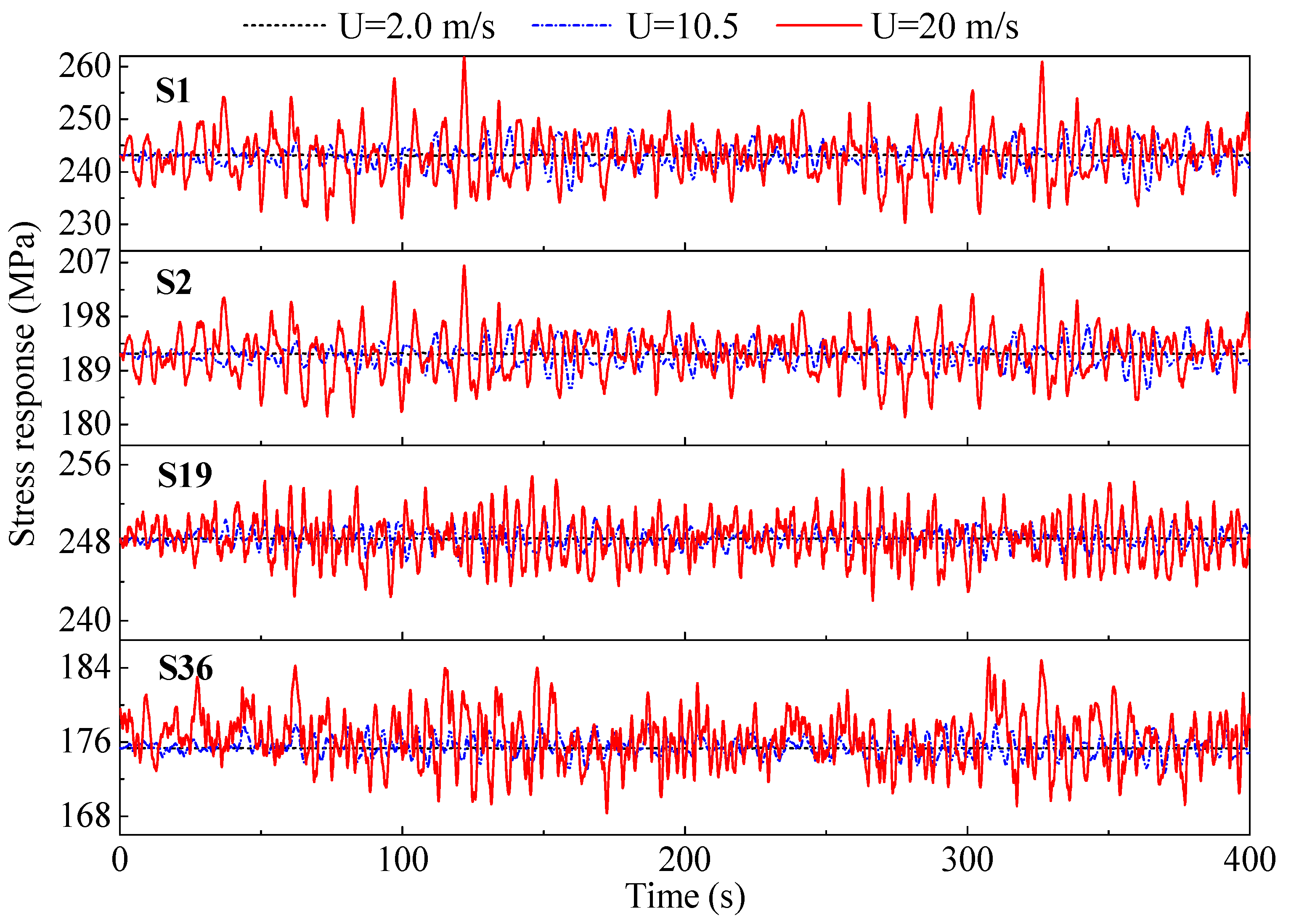
Considering the main focus of the present study is to predict the fatigue life of the suspenders, only the stress responses of the suspenders are presented and the discussion on dynamic responses of the bridge structure are not included herein. In this section, the stress responses of the representative suspenders resulting from individual wind load were first investigated, as shown in Figure 8. For better illustration, the stress responses for a duration of 400 s under the wind speeds of 2.0 m/s, 10.5 m/s, and 20 m/s are presented. For all the four representative suspenders, the variation of stress responses under lower wind speeds is much lower than that under higher wind speeds. Taking the suspender S1 as an example, the standard deviations of the stress responses under wind speeds of 2.0 m/s, 10.5 m/s, and 20 m/s were 0.07 MPa, 2.10 MPa, and 4.45 MPa, respectively. It is obvious that as the wind speed increases, the variation of the induced stress responses increases remarkably. Since the variation of the stress response relates to the stress range that directly determines the fatigue life, high winds are expected to be much more destructive in terms of fatigue reliability than the low winds.

As the prerequisite for estimating the fatigue life, the stress range values and number of cycles of all four representative suspenders were obtained through the rain-flow counting method, as listed in

Table 6. Stress ranges and number of stress cycles due to wind load in one day.

U	Equivalent Stress Range Values (MPa)				Numbers of Stress Cycles
	S1	S2	S19	S36	S1	S2	S19	S36
2.0 m/s	0.00	0.00	0.00	0.00	0	0	0	0
4.5 m/s	3.92	3.73	3.52	3.61	3168	2592	864	1296
7.5 m/s	5.12	4.82	3.97	4.12	6192	5328	1584	2880
10.5 m/s	7.71	6.86	4.06	4.19	10,080	8784	3312	5904
13.5 m/s	10.78	9.44	5.50	5.59	11,952	11,376	8064	12,240
16.5 m/s	15.28	12.88	7.37	8.67	14,256	12,960	10,368	14,544
20.0 m/s	15.79	13.61	7.79	9.46	17,424	15,408	17,280	18,144

. It is worth noting that the stress range cutoff levels have a strong effect on the number of cycles. In the present study, 3.45 MPa was chosen as the cutoff level for stress range to calculate the number of cycles, as the contribution of stress ranges less than 3.45 MPa can be neglected [35]. The results in Table 6 show that both the stress ranges and the number of stress cycles for all the selected suspenders under wind speed of 2.0 m/s were equal to 0, indicating that the contribution of U = 2.0 m/s to the fatigue damage of suspenders can be neglected. In addition, both the stress range and the number of cycles increase quickly with the increase of wind speed in general, showing that high wind speeds could cause much more significant fatigue damage to the suspenders than low wind speeds. This finding is consistent with the finding drawn from Figure 8.

5.2. Stress Ranges of Suspenders Resulting from Individual Traffic Load

Figure 9 displays the stress responses of the representative suspenders under both free-flow traffic and busy-flow traffic. It may be observed from Figure 9 that the stress level of the stress response for all four representative suspenders under free-flow traffic was at the same level as that under busy-flow traffic. However, the variation frequency of the stress response for all four representative suspenders under free-flow traffic was lower than that under busy-flow traffic, especially for short suspenders S19 and S36. This is due to the fact that the traffic volume of the busy-flow is more than 3 times that of the free-flow. With more vehicles in busy-flow passing by, the suspenders are expected to experience more truck passages, resulting in more rapid stress response variations. In addition, the short suspenders are believed to be more sensitive to the traffic loads than the long suspenders, because the influence of both the vertical and horizontal displacement at the anchor positions of short suspenders on their resultant stress responses are more appreciable. This can also explain why the stress response of short suspenders S19 and S36 under free-flow traffic displayed a distinctive pattern from that under busy-flow traffic.

The stress range values and number of cycles of all four representative suspenders under both free-flow and busy-flow traffic could be calculated based on the corresponding stress responses through the rain-flow counting method, as tabulated in

Table 7. Stress ranges and number of stress cycles due to traffic load in one day.

Traffic Condition	Equivalent Stress Range Values (MPa)				Numbers of Stress Cycles
	S1	S2	S19	S36	S1	S2	S19	S36
Free-flow	12.15	11.87	13.83	14.77	4896	4608	8352	9072
Busy-flow	12.53	12.05	13.89	14.87	7776	6624	15,984	18,576

. As shown in Table 7, the stress ranges for all selected suspenders under both types of traffic flow were very close (differences within 1.49%), while the number of cycles under busy-flow were remarkably larger than those under free-flow (increments range from 58.82% to 104.76%). This finding is also consistent with the finding observed from Figure 9. Furthermore, by comparing the results shown in Table 6 and Table 7, the stress range, as well the number of cycles under wind speed larger than 13.5 m/s, is comparable to those under traffic load, indicating that both wind and traffic play significant roles in predicting the fatigue life of suspenders.

5.3. Stress Ranges of Suspenders Resulting from Combined Wind and Traffic Loads

In this section, the stress ranges of suspenders under combined wind and traffic loads are investigated. The aforementioned discussions show that the stress responses of long suspenders, i.e., S1 and S2 were similar, while the stress response of short suspenders, i.e., S19 and S36, were similar. Therefore, the stress responses of long suspender S1 and short suspender S36 under combined wind and traffic loads are presented for demonstration purpose, as shown in Figure 10. It is shown in Figure 10a,b that, for both suspenders S1 and S36, the traffic load generally controls the mean trend of the stress response, while the wind load generally contributes to the fluctuation of the stress response. Consequently, as the wind speed increases, the fluctuation of the stress response increases remarkably. Therefore, it is clearly shown in Figure 10 that the stress responses of the suspenders under combined wind and traffic loads were larger than those under either individual wind load or individual traffic load. Considering that both the wind and traffic loads exist on the bridge during its life time, it is of paramount importance to account for both wind and traffic loads for the fatigue reliability analysis of suspenders.

Table 8. Stress ranges and number of stress cycles due to combined wind and traffic loads in one day.

Traffic Condition	Wind Speed	PT, i·PW, j1	Equivalent Stress Range Values (MPa)				Numbers of Stress Cycles
			S1	S2	S19	S36	S1	S2	S19	S36
Free-flow	0 2	0.145	12.15	11.87	13.83	14.77	4896	4608	8352	9072
	2.0 m/s	0.054	14.02	11.64	13.87	14.74	5328	5904	8352	10,224
	4.5 m/s	0.143	13.71	11.18	13.40	14.74	5184	5904	8352	10,080
	7.5 m/s	0.163	13.00	11.51	13.54	14.86	6192	6048	8496	10,080
	10.5 m/s	0.053	12.25	10.92	13.65	14.91	8352	7776	8928	10,224
	13.5 m/s	0.019	13.07	11.73	13.42	14.89	11,952	10,656	11,664	12,528
	16.5 m/s	0.006	15.87	13.97	13.60	16.25	13,824	12,096	13,536	15,408
	20.0 m/s	0.0001	17.19	14.34	13.37	14.44	16,992	16,128	19,008	18,288
Busy-flow	0 2	0.104	12.53	12.05	13.89	14.87	7776	6624	15,984	18,576
	2.0 m/s	0.039	13.78	12.92	11.84	13.00	8784	9216	15,408	19,296
	4.5 m/s	0.103	13.78	12.92	11.84	13.00	8784	9216	15,408	19,296
	7.5 m/s	0.116	13.48	13.04	11.72	13.05	9648	9360	15,120	19,152
	10.5 m/s	0.038	14.96	13.48	11.89	13.06	9936	10,224	14,400	18,288
	13.5 m/s	0.014	15.76	14.16	11.85	13.73	11,952	10,944	16,848	19,872
	16.5 m/s	0.004	17.33	14.85	12.84	14.95	13,680	12,960	16,704	19,728
	20.0 m/s	0.00004	18.39	16.02	12.86	15.68	17,136	15,120	19,440	21,024

¹P_{T, i}·P_{W, j} represents the probability occurrence of combined wind and traffic load as indicated in Equation (13). ² For comparison purpose, the no wind condition (U = 0) is also included in Table 8.

lists the stress ranges and number of stress cycles of four representative suspenders due to combined wind and traffic loads in one day. Based on the results in Table 8, the effective stress range ($S_{re}^{*}$) and the average daily number of cycles ($N_{avg}^{*}$) were then computed using Equations (13) and (14), as tabulated in

Table 9. Predicted effective stress range and average daily number of cycles.

	S1	S2	S19	S36
Predicted effective stress range (MPa)	13.32	12.13	13.14	14.33
Predicted average daily number of cycles	7278	7183	11,474	13,773

. The $S_{re}^{*}$ and $N_{avg}^{*}$ were further used to predict the fatigue life of the suspenders, as discussed in the subsequent section.

5.4. Fatigue Life Predictions

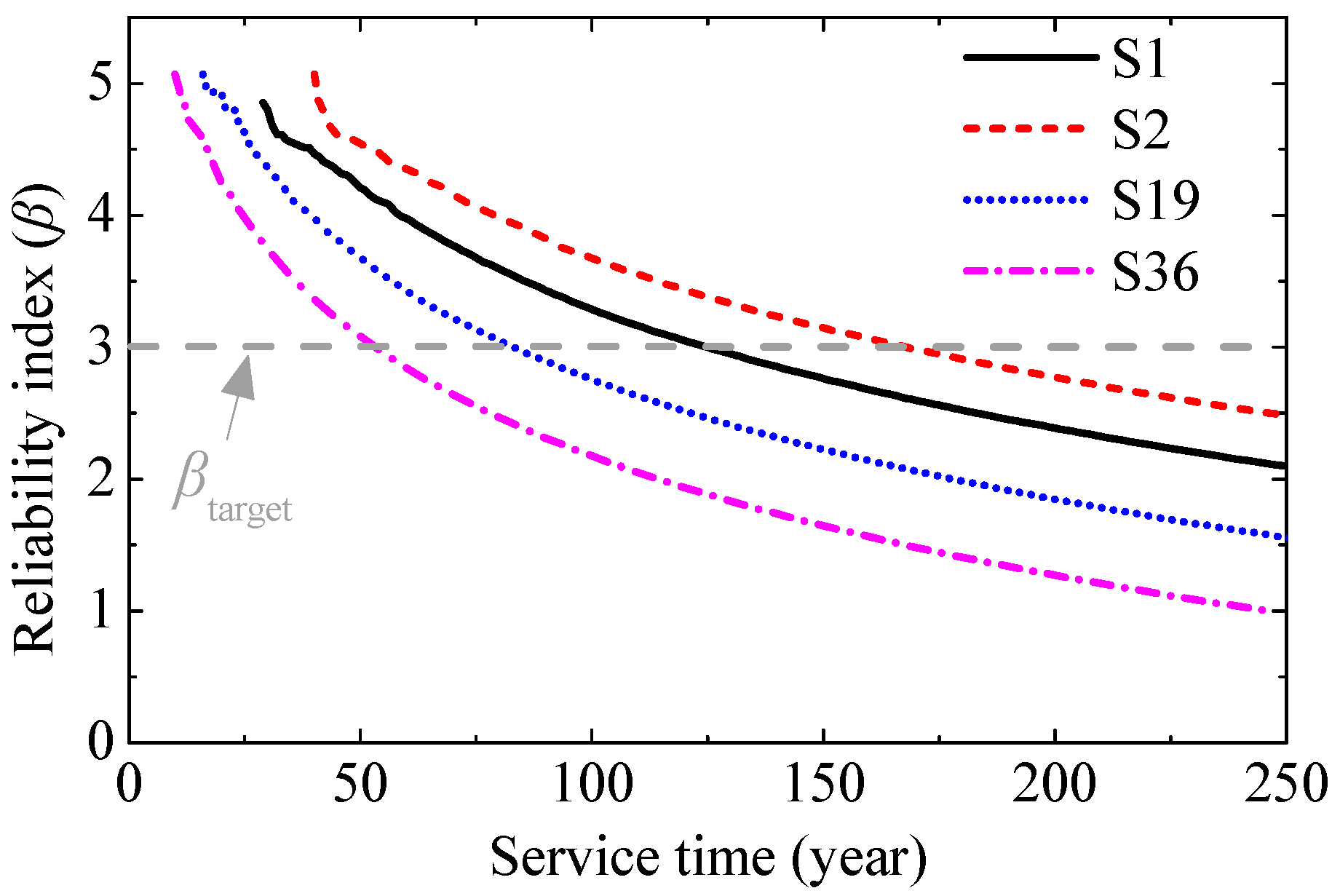
The predicted effective stress range and average daily number of cycles provides a reasonability basis for the fatigue reliability evaluation of the suspenders. In addition, the other random variables and constants that contribute to the fatigue damage are listed in Table 5. With the limit-state function shown in Equation (16) and the statistics of the random variables displayed in Table 6, the fatigue reliability index of each suspender of interest could be computed using Monte-Carlo simulations, as shown in Figure 11. It was observed that, among four suspenders under investigation, the short suspender S36 (mid-span suspender) and the long suspender S2 (girder end suspender) were, respectively, the most and the least prone to fatigue damage. If the service life of the suspender is designed as 100 years, the corresponding reliability indices for suspenders S1, S2, S19, and S36 are reduced to 3.28, 3.68, 2.76, and 2.18, respectively.

Furthermore, the fatigue life can be estimated provided with a target reliability (β_target). Since, currently, no consensus has been reached in the literature regarding the target reliability for the suspenders, the value of 3.0 was adopted in the present study, which corresponds to a failure probability of 0.135%. As a result, the fatigue life of the representative suspenders S1, S2, S19, and S36 under β_target was calculated as 124 years, 167 years, 83 years, and 53 years, respectively.

6. Conclusions

In the present study, the time-dependent fatigue reliability of the suspenders considering life time stochastic wind and traffic loads was evaluated based on fully coupled traffic-bridge-wind (TBW) analysis. In order to accurately predict the fatigue reliability of the suspenders, the in-situ monitoring data containing the essential wind and traffic information were analyzed thoroughly first and then subsequently implemented into the stochastic wind and traffic model. Finally, the linear fatigue damage rule was adopted to estimate the fatigue life of the suspenders. The following conclusions could be drawn:

(1)

If only the wind load is considered, the results indicate that high wind speeds could cause much more significant fatigue damage on the suspenders than low wind speeds.

(2)

If only the traffic load is considered, it was found that the stress level of the stress response of the suspenders under free-flow traffic is at the same level as that under busy-flow traffic. However, the variation frequency of the stress response of suspenders is lower than that under busy-flow traffic, especially for short suspenders S19 and S36.

(3)

Considering both wind and traffic loads, it was indicated by the stress responses of the suspenders that both wind and traffic play significant roles in predicting the fatigue life of suspenders.

(4)

The short suspender S36 (mid-span suspender) and the long suspender S2 (girder end suspender) were, respectively, the suspenders most and the least prone to fatigue damage. In addition, provided with a target reliability index of 3.0 and considering the lifetime wind and traffic load, the fatigue life of suspenders S36 and S2 was estimated at 53 years and 167 years, respectively.

In the present study, only the portion of the suspender away from the structural connections, e.g., anchor zone, was investigated. The portion of the suspender near or located at the structural connections is subjected to very complex stress status including tension, bending, or even shear and torsion. Under such complex stress status, a more sophisticated methodology, e.g., fracture mechanics probably combined with very refined finite element modeling, may be required to evaluate the fatigue damage and predict the fatigue life of the suspender, which is currently under investigation by the authors.

References

1. Morcillo, M.; Chico, B.; Díaz, I.; Cano, H.; de la Fuente, D. Atmospheric corrosion data of weathering steels. A review. Corros. Sci. 2013, 77, 6–24. [Google Scholar] [CrossRef] [Green Version]
2. Xu, Y.L. Wind Effects on Cable-Supported Bridges, 1st ed.; John Wiley & Sons Singapore: Singapore, 2013; ISBN 9788578110796. [Google Scholar]
3. Zhu, J.; Zhang, W.; Zheng, K.F.; Li, H.G. Seismic design of a long-span cable-stayed bridge with fluid viscous dampers. Pract. Period. Struct. Des. Constr. 2015, 21, 04015006. [Google Scholar] [CrossRef]
4. Zhu, J.; Zhang, W. Coupled analysis of multi-impact energy harvesting from low-frequency wind induced vibrations. Smart Mater. Struct. 2015, 24, 045007. [Google Scholar] [CrossRef]
5. Pham, V.L.; Ha, N.S.; Goo, N.S.; Choo, J.F. Effects of cyclic impacts on the performance of a piezo-composite electricity generating element in ad 33 mode energy harvesting. J. Nanosci. Nanotechnol. 2014, 14, 7410–7418. [Google Scholar] [CrossRef] [PubMed]
6. Hopwood, T.; Havens, J.H. Inspection, Prevention, and Remedy of Suspension Bridge Cable Corrosion Problems; Kentucky Transportation Cabinet: Lexington, KY, USA, 1984. [Google Scholar]
7. Zheng, X.; Xie, X.; Li, X. Experimental study and residual performance evaluation of corroded high-tensile steel wires. J. Bridg. Eng. 2017, 22, 04017091. [Google Scholar] [CrossRef]
8. Hopwood, T.; Havens, J. Corrosion of Cable Suspension Bridges; Kentucky Transportation Cabinet: Lexington, KY, USA, 1984. [Google Scholar]
9. Li, H.; Lan, C.M.; Ju, Y.; Li, D.S. Experimental and numerical study of the fatigue properties of corroded parallel wire cables. J. Bridg. Eng. 2012, 17, 211–220. [Google Scholar] [CrossRef]
10. Xu, J.; Chen, W. Behavior of wires in parallel wire stayed cable under general corrosion effects. J. Constr. Steel Res. 2013, 85, 40–47. [Google Scholar] [CrossRef]
11. Liu, Z.; Guo, T.; Chai, S. Probabilistic fatigue life prediction of bridge cables based on multiscaling and mesoscopic fracture mechanics. Appl. Sci. 2016, 6, 99. [Google Scholar] [CrossRef]
12. Liu, Z.; Guo, T.; Hebdon, M.H.; Zhang, Z. Corrosion fatigue analysis and reliability assessment of short suspenders in suspension and arch bridges. J. Perform. Constr. Facil. 2018, 32, 04018060. [Google Scholar] [CrossRef]
13. Li, S.; Zhu, S.; Xu, Y.; Chen, Z.; Li, H. Long-term condition assessment of suspenders under traffic loads based on structural monitoring system: Application to the Tsing Ma Bridge. Struct. Control Health Monit. 2012, 19, 82–101. [Google Scholar] [CrossRef]
14. Liu, Z.; Guo, T.; Huang, L.; Pan, Z. Fatigue life evaluation on short suspenders of long-span suspension bridge with central clamps. J. Bridg. Eng. 2017, 22, 04017074. [Google Scholar] [CrossRef]
15. Deng, Y.; Li, A.; Feng, D. Fatigue performance investigation for hangers of suspension bridges based on site-specific vehicle loads. Struct. Health Monit. 2019, 18, 934–948. [Google Scholar] [CrossRef]
16. Zhu, J.; Zhang, W. Probabilistic fatigue damage assessment of coastal slender bridges under coupled dynamic loads. Eng. Struct. 2018, 166, 274–285. [Google Scholar] [CrossRef]
17. Nagel, K.; Schreckenberg, M. A cellular automaton model for freeway traffic. J. Phys. I 1992, 2, 2221–2229. [Google Scholar] [CrossRef]
18. Zhou, Y.; Chen, S. Framework of Nonlinear Dynamic Simulation of Long-Span Cable-Stayed Bridge and Traffic System Subjected to Cable-Loss Incidents. J. Struct. Eng. 2015, 142, 04015160. [Google Scholar] [CrossRef]
19. Wu, J. Reliability-Based Lifetime Performance Analysis of Long-Span Bridge. Ph.D. Thesis, Colorado State University, Fort Collins, CO, USA, 2010. [Google Scholar]
20. Hou, G.; Chen, S.; Han, Y. Traffic performance assessment methodology of degraded roadway links following hazards. J. Aerosp. Eng. 2019, 32, 04019055. [Google Scholar] [CrossRef]
21. Chen, S.R.; Wu, J. Dynamic Performance Simulation of Long-Span Bridge under Combined Loads of Stochastic Traffic and Wind. J. Bridg. Eng. 2010, 15, 219–230. [Google Scholar] [CrossRef]
22. Zhu, J.; Zhang, W.; Wu, M. Evaluation of ride comfort and driving safety for moving vehicles on slender coastal bridges. J. Vib. Acoust. ASME 2018, 140, 051012. [Google Scholar] [CrossRef]
23. Zhu, J.; Zhang, W.; Wu, M. Coupled dynamic analysis of vehicle-bridge-wind-wave system. J. Bridg. Eng. 2018, 23, 1–17. [Google Scholar] [CrossRef]
24. Wu, M.; Li, Y.; Chen, X.; Hu, P. Wind spectrum and correlation characteristics relative to vehicles moving through cross wind field. J. Wind Eng. Ind. Aerodyn. 2014, 133, 92–100. [Google Scholar] [CrossRef]
25. Wu, M.; Li, Y.; Zhang, W. Impacts of wind shielding effects of bridge tower on railway vehicle running performance. Wind Struct. 2017, 25, 63–77. [Google Scholar]
26. Lin, Y.K.; Yang, J.N. Multimode Bridge Response to Wind Excitations. J. Eng. Mech. 1983, 109, 586. [Google Scholar] [CrossRef]
27. Baker, C.J. A simplified analysis of various types of wind-induced road vehicle accidents. J. Wind Eng. Ind. Aerodyn. 1986, 22, 69–85. [Google Scholar] [CrossRef]
28. Wang, H.; Li, A.; Hu, R. Comparison of ambient vibration response of the Runyang suspension bridge under skew winds with time-domain numerical predictions. J. Bridg. Eng. 2011, 16, 513. [Google Scholar] [CrossRef]
29. AASHTO LRFD Bridge Design Specifications, 6th ed.; American Society of Civil Engineers: Washington, DC, USA, 2012; ISBN 9781560514510.
30. European Committee for Standardization. Design of Steel Structures; Fatigue: Brussels, Belgium, 2005. [Google Scholar]
31. Miner, M.A. Cumulative damage in fatigue. J. Appl. Mech. 1945, 12, 159–164. [Google Scholar]
32. Kwon, K.; Frangopol, D.M.; Kim, S. Fatigue performance assessment and service life prediction of high-speed ship structures based on probabilistic lifetime sea loads. Struct. Infrastruct. Eng. 2013, 9, 102–115. [Google Scholar] [CrossRef]
33. Wirsching, P.H. Fatigue reliability for offshore structures. J. Struct. Eng. 1984, 110, 2340–2356. [Google Scholar] [CrossRef]
34. Niu, H.; Zhu, J.; Chen, Z.; Zhang, W. Dynamic performance of a slender truss bridge subjected to extreme wind and traffic loads considering 18 flutter derivatives. J. Aerosp. Eng. 2019. [Google Scholar] [CrossRef]
35. Kwon, K.; Frangopol, D.M. Bridge fatigue reliability assessment using probability density functions of equivalent stress range based on field monitoring data. Int. J. Fatigue 2010, 32, 1221–1232. [Google Scholar] [CrossRef]
Figure 1. Numerical model of a 3-axle vehicle: (a) Elevation view; (b) side view.
Applsci 09 03405 g001
Figure 2. Wind rose diagrams: (a) Mean wind velocity (m/s); (b) probability of occurrence of wind direction.
Applsci 09 03405 g002
Figure 3. Hourly traffic volume: (a) Fast lane; (b) slow lane.
Applsci 09 03405 g003
Figure 4. Simulated stochastic traffic flow. (a) Fast-lane: Free-flow; (b) fast-lane: Busy-flow; (c) slow-lane: Free-flow; and (d) slow-lane: Busy-flow.
Applsci 09 03405 g004
Figure 5. Comparison between the predicted distribution of the gross vehicle weight of various vehicle types in the simulated stochastic traffic flow and the target distribution (a) V1, (b) V3, (c) V5, and (d) V7.
Applsci 09 03405 g005
Figure 6. Layout of the prototype suspension bridge (m).
Applsci 09 03405 g006
Figure 7. Wire rope suspenders (a) configuration and (b) cross sections.
Applsci 09 03405 g007
Figure 8. Segment of stress response time histories of representative suspenders under various wind speeds.
Applsci 09 03405 g008
Figure 9. Segment of stress response time histories of representative suspenders under individual traffic load.
Applsci 09 03405 g009
Figure 10. Segment of stress response time histories of representative suspenders under combined wind and traffic load (a) suspender S1 and (b) suspender S36.
Applsci 09 03405 g010
Figure 11. Fatigue reliability index of the four representative suspenders.
Applsci 09 03405 g011