Article

Modeling of the Snowdrift in Cold Regions: Introduction and Evaluation of a New Approach

1
Key Lab of Structures Dynamic Behavior and Control of the Ministry of Education, Harbin Institute of Technology, Harbin 150090, China
2
Key Lab of Smart Prevention and Mitigation of Civil Engineering Disasters of the Ministry of Industry and Information Technology, Harbin Institute of Technology, Harbin 150090, China
*
Author to whom correspondence should be addressed.
Appl. Sci. 2019, 9(16), 3393; https://doi.org/10.3390/app9163393
Submission received: 17 July 2019 / Revised: 14 August 2019 / Accepted: 14 August 2019 / Published: 17 August 2019
(This article belongs to the Special Issue Buildings and Structures under Extreme Loads)

Abstract

:

Featured Application

A new approach for investigating snowdrifts around buildings and snow loads on building roofs based on a new facility named the “snow–wind combined experimental facility” is proposed in this paper. First, the method proposed in this paper is convenient and economical, and also the experimental results prove that the method is feasible and reliable. In this paper, only experiments on snowdrift around a cube were chosen for the verification for the sake of generality, but this method could also be adopted for the prediction of snowdrift around complex building environments and snow loads on various shapes of building roofs.

Abstract

Unbalanced, or non-uniform, snow loads caused by snow drifting or sliding in cold regions with heavy snowfalls, can be a serious problem for the building industry. However, the methods for predicting snow distribution still need to be improved. Field observation is the most direct and reliable method to study snow distribution, but because the natural environment is uncontrollable and varies dramatically, sometimes conclusions may be confused under the influence of the many variables in the investigation. This paper proposes a snowing experiment approach using an outdoor snow–wind combined experiment facility for the study of snow distribution. The facility can produce a stable and controllable wind field and snowfall environment. Experiments which focused on snowdrift around a building were conducted during the winter to make an evaluation of the repeatability and reliability of the new approach. Finally, from the analysis of results, it was demonstrated that the experimental facility was stable and that the similarity criterion adopted for the snowing pattern was reliable. Especially, the minimum value of the friction speed ratio was suggested to ensure the test accuracy.

1. Introduction

Since ancient times, buildings have been constructed to protect people from the natural environment. The environment dictates what type of building should be constructed, and snow loads are one of the dominant live loads that should be considered in the design of buildings in cold regions with a severe winter climate. Investigations show that snow loads are usually unbalanced, due to the action of the wind. And snowdrifts around buildings may cause problems for the vehicular traffic and pedestrians.
Currently, field observations, numerical simulations, and wind tunnel tests are the three main methods to estimate snow distribution, and much work has been undertaken to explore how the wind affects snow distribution.
Field observation is the most direct and reliable approach for obtaining information on snow distributions. Investigations of snowdrifts around an isolated building or group of buildings have been carried out in several previous studies [1,2]. Thiis and Gjessing [3] investigated the snowdrifts around three different model buildings in a valley in Spitsbergen, Norway, and the results showed that a change of roof shape could lead to large differences in snow distribution around the building. Beyers et al. [4] carried out research to investigate the snowdrift around a 2.0 × 2.0 × 2.0 m3 cube at the SANAE IV research station, Antarctica, during the summer of January 2002 and verified the accuracy of a numerical simulation model using the results of field observations. Høibø [5,6] measured snow loads on nearly 200 building roofs under different wind and sun/shade environments from 1966 to 1986 in southern Norway. This method has strict requirements on the environment of the test site, such as wind velocity, temperature, humidity, and snowfall, but these important parameters in the observation were unstable and uncontrollable.
In 1991, Uematsu [7] first used numerical simulation to analyze snowdrifts, and now this method is widely used by researchers. Tominaga et al. [8] analyzed the snowdrift around an actual apartment building using the revised k-ε model. Beyers et al. [4] predicted transient snowdrift around a cubic structure using the standard k-ε model. And a large amount of numerical work has been done recently due to its significant advantage in efficiency and convenience [9,10,11,12]. However, only a few attempts have been made to apply CFD (Computational Fluid Dynamics) to roof loading so far [13]. Thiis et al. [14,15] predicted the snow distribution on a curved roof of a sports hall located in Oslo and compared the results with measurements. Some researchers are confused by the selection of the turbulence models, hence there is no approved and unified model.
Wind tunnel testing [16,17,18] is the most effective method for investigating snow distribution under the action of airflow. Kind [19,20] identified the important similarity criteria by analyzing the saltation process and discussed the necessary compromises in the modeling procedures. Delpech et al. [21] used artificial snow to simulate snow drifting around buildings for the Antarctic Concordia research station. Okaze et al. [22] investigated the development of drifting snow in a boundary layer wind tunnel. LÜ et al. [23] conducted a series of experiments in a wind tunnel to investigate the motion of natural snow and found that the threshold wind speeds for fresh and old snow were 6.2 m/s and 6.8 m/s (at 10 m height). Zhou et al. [24,25] investigated the snow distribution on a stepped flat roof using different granular materials in an open straight-circuit wind tunnel and also conducted a series of experiments on snow loads on flat roofs using high-density silica in the open test section of a boundary-layer wind tunnel. However, the snowdrift simulations in a boundary-layer wind tunnel struggle with scaling issues and similarity criteria. Some previous experiments on snowdrifts using wind tunnels have used bran, or other particles, as a substitute for natural snow, but these cannot completely replicate the distribution of natural snow. Tests have been carried out in advanced climate wind tunnels [26], where the influencing factors that may affect the results, such as the wind speed, temperature, and snowfall rate, are fully controllable. However, they are very expensive and not readily available for most researchers.
Snowdrift loads around buildings or on the roofs, which have a great impact on functionality and security of buildings, require particular attention. However, for the existing research methods, numerical simulation still needs to be improved with data from field observations and wind tunnel tests. Field observations are rarely available when considering security and technical issues, even though they should provide the most reliable data. Wind tunnel tests are the main source of data, but the expense of experiments in climate wind tunnels is so high that few experiments are reported, and it has restricted further studies. What is more, the wind speed and direction of field observations vary dramatically, so some conclusions may be confused when the natural environment is problematic. Hence, this paper proposes a new approach to investigate the snowdrift loads with a facility in which the wind speed and direction are controllable and a snowing environment, just like natural snowfall, is available.
The purpose of this facility is to provide a new approach to study snow distribution under the action of wind. In comparison with traditional wind tunnel tests, there will be a 90% or more decrease in the construction cost because the facility need not be equipped with a refrigerating system. Besides that, the operating expense of the facility is much lower than climate wind tunnels.
Transportation of snow particles can be classified into three processes, i.e., creep, saltation, and suspension. Saltation, which is widely accepted as contributing most to the total transfer volume, is a process in which snow particles move with repeated leaping up, or jumping, on the snow surface.
The height of saltation is usually below 0.1 m. Generally, the length of saltation L [27] is suggested to be
L 10   h .
Yet, to ensure that the saltation process could be accurately reproduced on the roofs or around the building, it is suggested that the characteristic length of the prototype model is larger than the length of saltation L.
In this study, the design parameters of the facility, experiment method, and the adopted similarity criteria are introduced and discussed. Finally, a prototype model with external dimensions of 1.0 × 1.0 × 1.0 m3 was selected, taking both economy and theory into consideration, to study the surrounding snow distribution and evaluate the repeatability and reliability of the new approach.

2. Design of the Snow–Wind Combined Experiment Facility

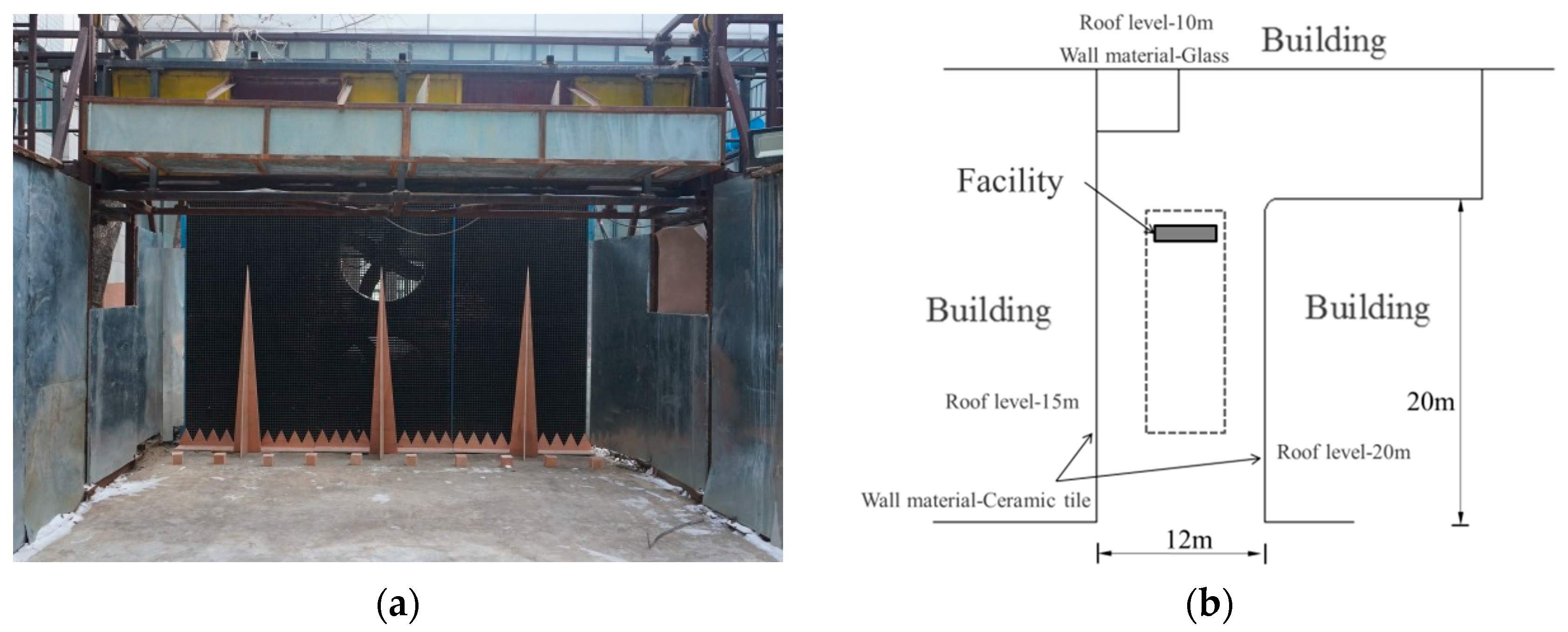
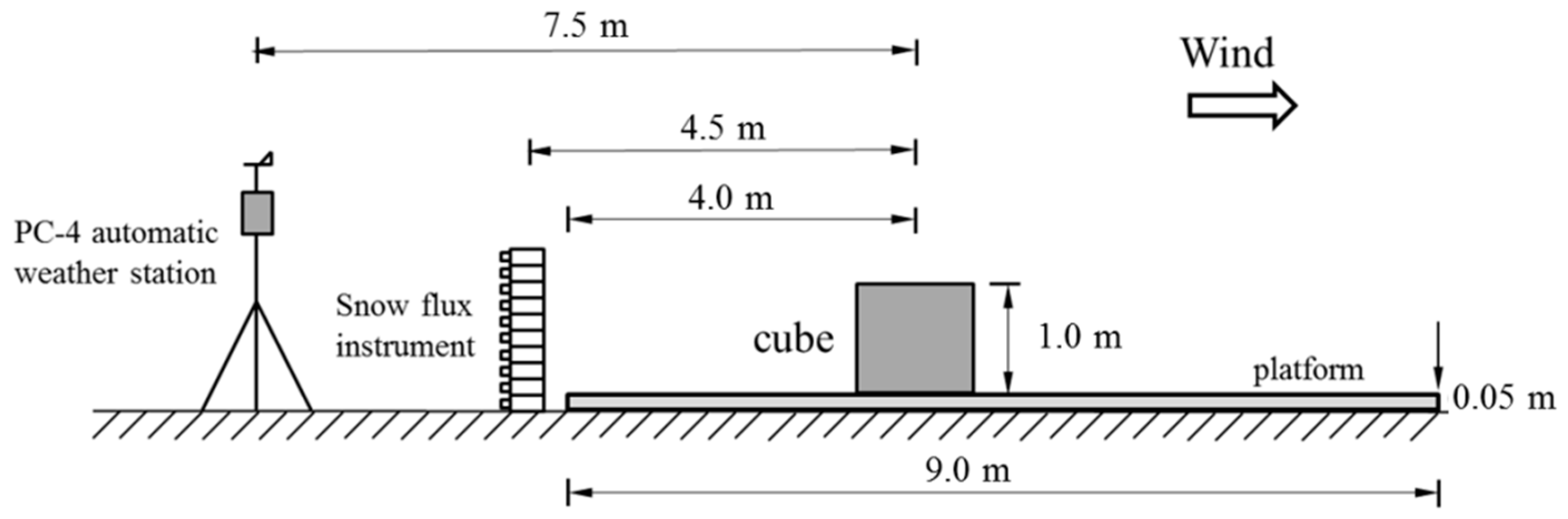
2.1. Brief Introduction of the Facility

In the study of snow distribution, numerical simulations and wind tunnel tests should be verified by field observations. For this purpose, a snow–wind combined experiment facility as shown in Figure 1a has been constructed at the Harbin Institute of Technology (HIT) to produce stable wind fields to investigate snow distribution [28] The climatic characteristics of the winter months in Harbin provide convenient conditions for the experiments. Harbin has a long winter, which can last for almost six months, with snowy conditions and a temperature range from −30 °C to 0 °C. The location of the facility is shown in Figure 1b. Because the facility was to be sited outdoors, a narrow strip between two buildings was chosen to reduce the interference of the external environment. The dimension of available ground is 12 m × 20 m, and the heights of the surrounding buildings are all greater than 10 m.

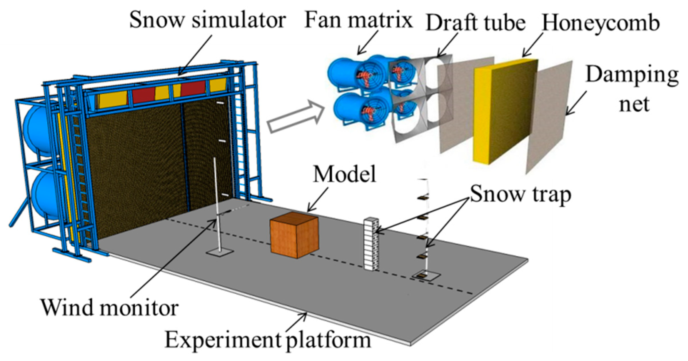
2.2. Introduction of the Main Component

The facility, as shown in Figure 2, consists of a power section, a flow conditioning section, an experimental section, and a snowfall simulator.
The power station is the 3 × 2 fan-matrix, and the area affected by the model during a snowdrift is thought to be about three times larger than the characteristic length of the model [27]. Therefore, the cross-section of the facility was designed to be 4.5 × 3.0 m2. Considering the fact that there are usually light winds when it is snowing, the facility was designed to be able to produce a stable wind field for a specific duration with a range of speeds from 0.5 to 11.5 m/s. Wind pressure is the main indicator of the output of the fan-matrix and is defined as
P = ρ k U 0 2 2 ,
where P is the wind pressure; ρ is the density of air, and ρ = 1.395 kg/m3 when the temperature is −20 °C; k is the resistance coefficient of pressure of the flow conditioning section, which is defined as the ratio of the outlet area of the facility to the total outlet area of the six airflow fans, and k = 1.734; U0 is the wind speed at the outlet or immediate output from the fan matrix, and Umax, which is measured at the section 4 m away from the outlet, is regarded as the available maximal wind speed of the facility and Umax = 11.5 m/s for design purposes.
Because the facility is open to the natural environment, a numerical simulation was undertaken to explore the relationship between U0 and U, where U is the wind speed at the experiment section. Based on the environment of the experimental site, a calculation model of the facility, with a computational domain of 10 × 10 × 20 m3, was formulated. The result showed that when the initial velocity of the wind export of the facility was 15 m/s, the uniform wind speed in the range of 4–20 m was about 11.5 m/s, hence, the value of U0 is approximately equal to 15 m/s.
Accordingly, the minimum wind pressure is 272.1 Pa by calculation, and a fan with 286 Pa wind pressure was chosen. The maximum speed measured in the field was 11.5 m/s, which reasonably meets the requirements of the experiments.
The flow conditioning section, which stabilizes and smooths the airflow produced by the fan, is a combination of the draft tube, the honeycomb, and the damping net. Two pieces of damping net were stuck on both import and export sections of the honeycomb, and the draft tube served as connection between the power section and the honeycomb. The flow conditioning section was designed to be short to reduce the loss of wind power because of the open experimental environment. Considering the square pattern of the cross-section and the design experience from the wind erosion tunnel designed by Saxton [29], a square cross-section with the dimension of 30 × 30 mm2 was chosen as the single unit of the honeycomb with a length of 300 mm. The experimental section is a platform with a circular dial, which is used to fix the model at the required angle.
Snowfall suitable for the experiments was not always available, so to accumulate a large amount of data on snow distribution, it was necessary to find a way to simulate snowfall using natural or artificial snow particles.
In this work, a snowfall simulator situated 1 m away from the wind export was designed to simulate snowfall during the experiments. Before the experiments started, snow, which had been collected in heat-insulation boxes, was placed in a metal box with wire gauze on the bottom. Then, shaking the metal box with an eccentric motor to generate friction between the snow and wire gauze, made snow particles fall from the mesh into the stable wind field caused by the fan-matrix so that a snowfall environment was formed in the test section. Different snowfall conditions are available using different kinds of wire gauze with varied vibration frequency. There are three different kinds of the aperture of wire gauze, 2 mm, 3 mm, and 5 mm, and the vibration frequency ranges from 1 to 5 Hz. The metal box, which is 5 m wide, can be raised and lowered freely in the range of 0.5–3 m.

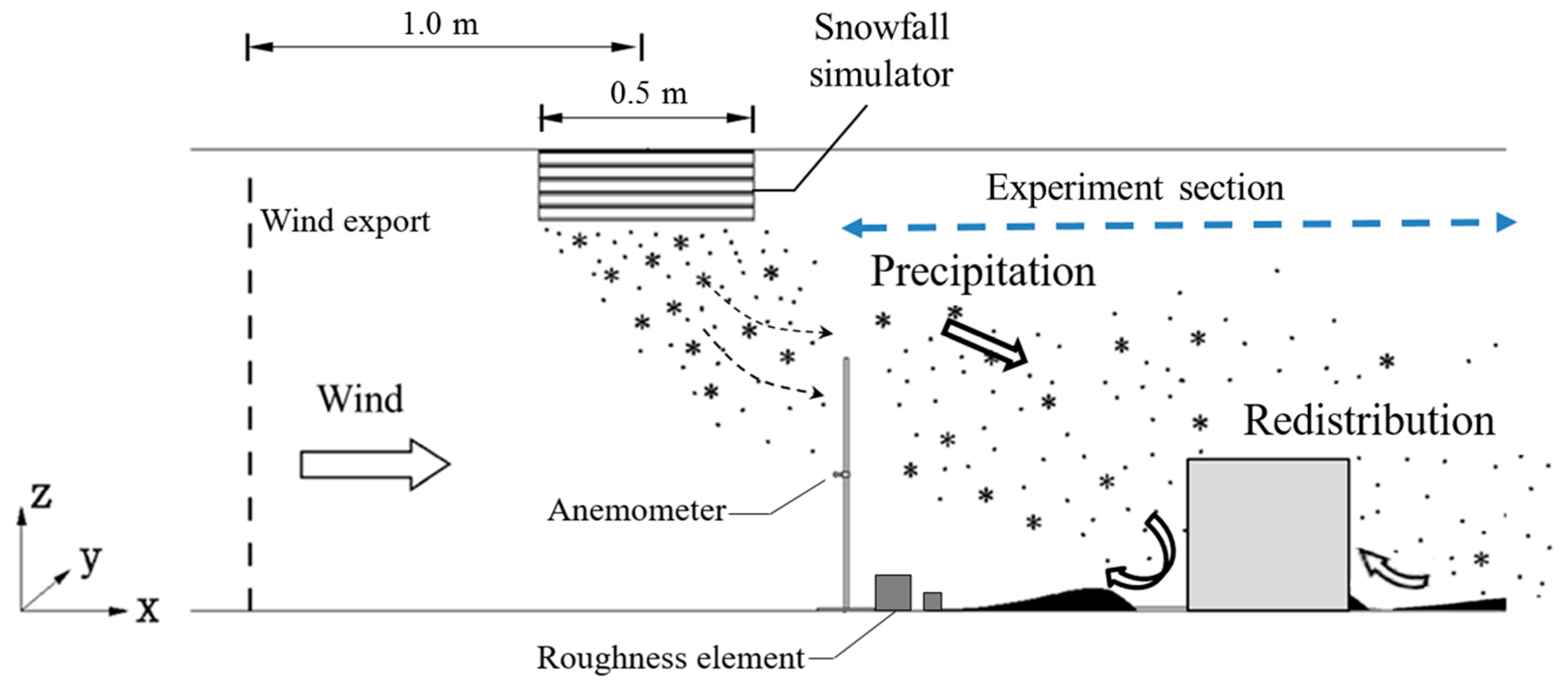
2.3. A Brief Introduction to the Experimental Procedure

Figure 3 shows a sketch of the experimental procedure. The facility can provide a controlled snowfall environment in the test section so that experiments examining snow distribution around the building or on roofs can be undertaken.
When an experiment is going to be conducted, there are four steps: First of all, enough snow should be put into the box of the snow simulator, next the model should be fixed according to the experiment design along with an anemograph for monitoring the wind speed at the reference point; then the fan-matrix is started and adjusted until the wind speed reaches a given value, and then the snow simulator can be turned on for the required duration; finally, the snow load is measured after all of the equipment has been turned off.

3. Verification of the New Approach

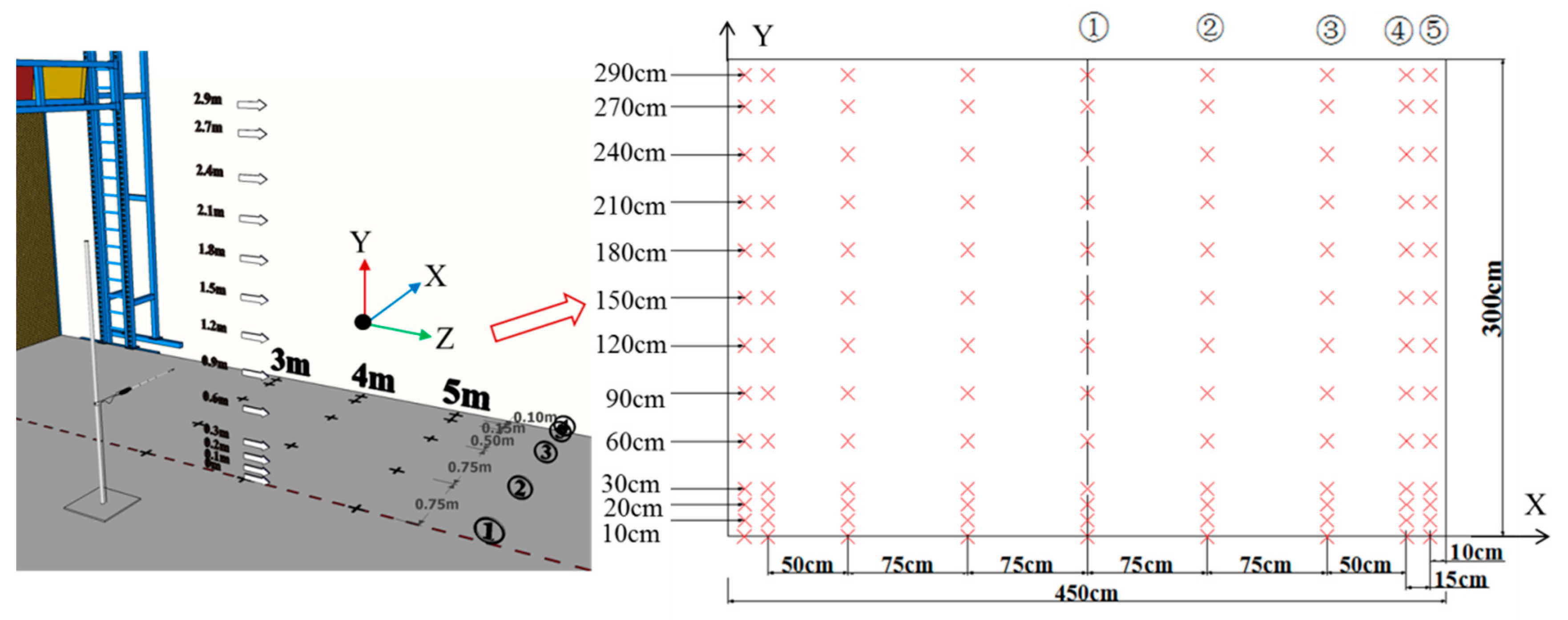
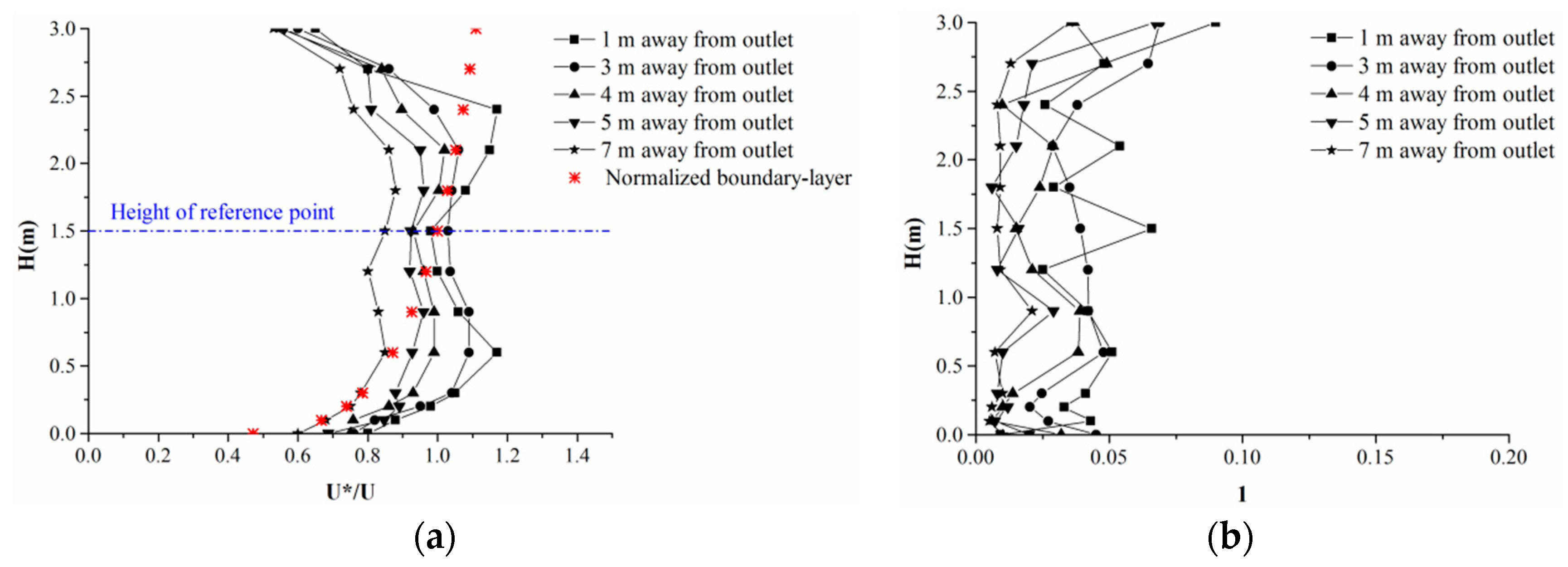
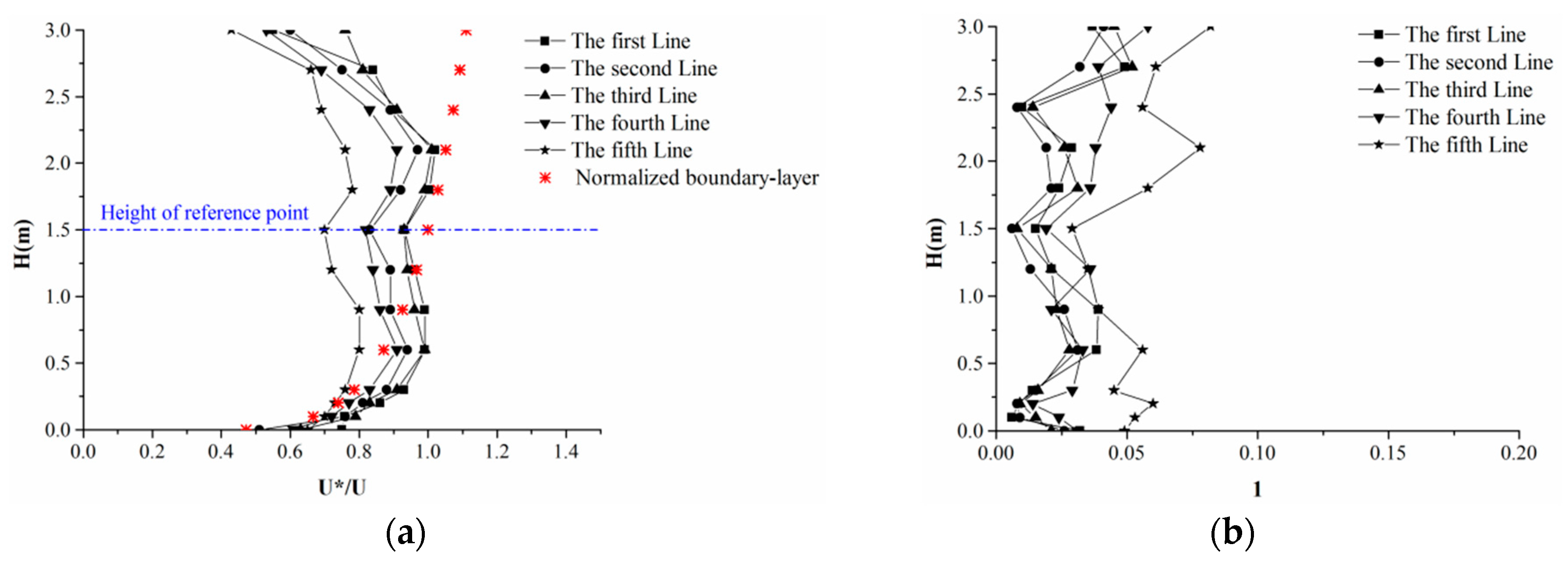
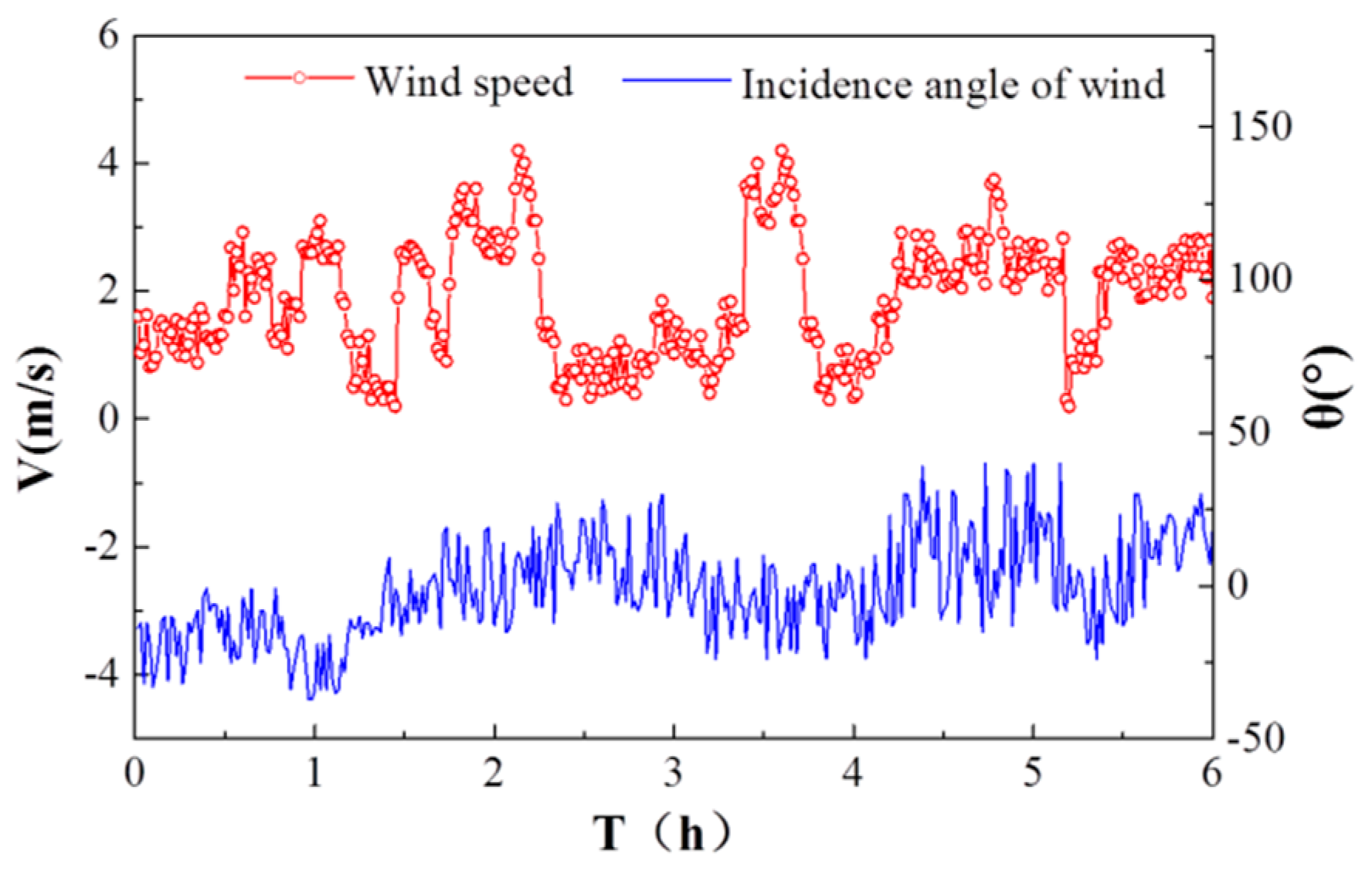
3.1. Field Measurements of Wind Field Produced by the Facility

Obviously, the wind field has a significant impact on the results of the experiments, so field measurements of the actual wind field were also made to investigate it and determine the best location of the experimental platform.
Figure 4 shows the method for measuring the wind field. Because the cross-section is symmetrical, the measuring points are arranged symmetrically in the full section. The wind speed was measured by a hot-wire Thermo-Anemometer and each measuring point was measured at least 30 s with a sampling frequency of 1 Hz. The vertical and horizontal measurement points in each cross-section formed a matrix of 13 × 9. Before the measurements, a design speed U was defined. If the measured wind speeds at the 1.5 m point on the first line of the five sections were all between 0.9~1.1 U, this would be recognized as the design speed U. Five cross-sections were measured with a design speed (U) of 3.0 m/s and the distance between them and the export was 1 m, 3 m, 4 m, 5 m, and 7 m.
Figure 5a shows that the mean wind speed on the first line of five cross-sections varies with height; the Y-axis represents the height of the cross-section and the X-axis represents the ratio between U* (the measured wind speed) and U. Figure 5b shows the turbulence intensity of wind on each measuring point. It is apparent that the turbulence intensity is higher in the section before 3 m and the wind is more uniform in the range 3–7 m; this was also shown in the numerical simulation. However, the wind speed decreased faster with increasing distance from the export, which is slightly different from the numerical simulation. To ensure a stable and uniform wind field during the experiments, the effective range of the experimental section was 3–7 m away from the wind export.
Figure 6a shows how the mean wind speed varies with width in the cross-section 4 m away from the export, and Figure 6b shows the turbulence intensity of wind on each measuring point. And from the results, it is apparent that the wind speed decreased rapidly close to the edge of the cross-section. To ensure the veracity of the experiments, the effective width of the experimental section was 4 m.
From a comparison of the measured wind speed with the normalized wind speed in the atmospheric boundary layer, the discrepancy above 1.5 m is non-negligible, but it is relatively acceptable for the given experiment. The turbulence intensity was small except at some points close to the wind export and at the edges of the cross-section, which indicates that the quality of the flow field in the open test section was reasonable and acceptable.
During the experiments, temperature, the natural wind field, and humidity were measured on a PC-4 automatic weather station, which is located on the side of the facility, to rectify the experimental wind field. This has three anemometers, at heights of 0.5 m, 1.5 m, and 2.0 m, and the sampling interval was 1 min.

3.2. Physical Properties of Snow

Properties of snow particles have a great influence on the result of the test [23] so that the physical properties of the stored natural snow particles were measured before the experiments. The diameter and shape of the snow particles were observed by an optical microscope and the angle of repose was decided from accumulated experimental observations. The terminal velocity of the snow particles was decided by measuring the time that the snow particles freely fell from 2 m to the ground level. A comparison of the physical parameters of the snow particles is given in Table 1.

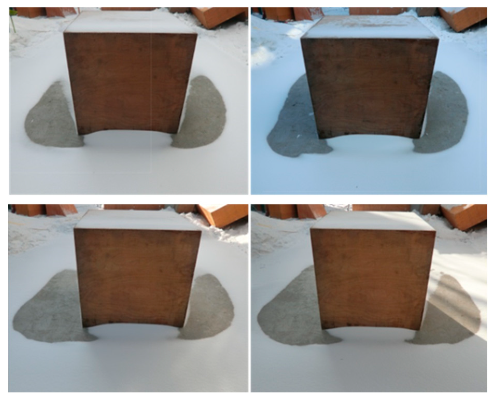
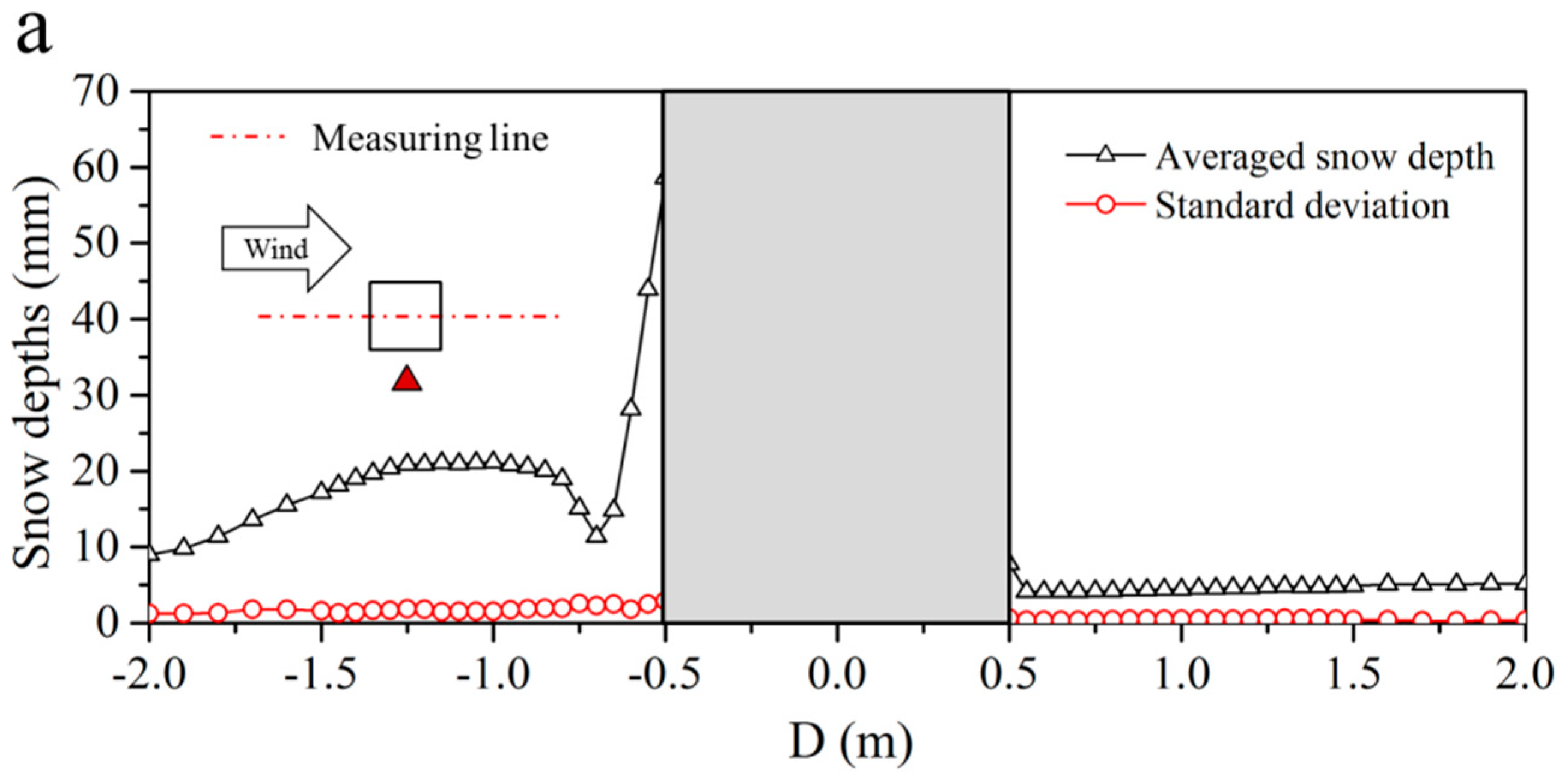
3.3. Experiments for the Verification of Repeatability

To confirm the repeatability of the new approach, 20 repetitive experiments using stored snow on the snowdrift surrounding a 1 m cube were undertaken. Environmental conditions, namely temperature, humidity, and natural wind field were measured by an automatic weather station that was sited nearby the test section and results are shown in Table 2. The reference point for the experimental wind speed was set at 1 m in front of the model and 0.5 m above the ground. The snowing rate was defined as the accumulated snow depth on the ground in unit time and it was determined by the kind of wire gauze and vibration frequency. For the 20 experiments, the snowing rate was controlled to be the same. Figure 7 shows some photos of the experiment results.
Figure 8 gives the distribution of average snow depth and the standard deviation of each measured point along lateral and streamwise lines crossing the model. It is clear that the distribution of snow depths in the 20 experiments is relatively stable. The Pearson Correlation Coefficient for any two experimental results along the measuring lines shown in Figure 8 was above 0.90, which indicates that there is a strong correlation between the results from the 20 experiments.
From the above analysis, it can be concluded that the results of the 20 experiments, with the same test conditions, show good correspondence with each other. This indicates that the method provides good stability and repeatability.

3.4. Experiments for the Verification of Reliability

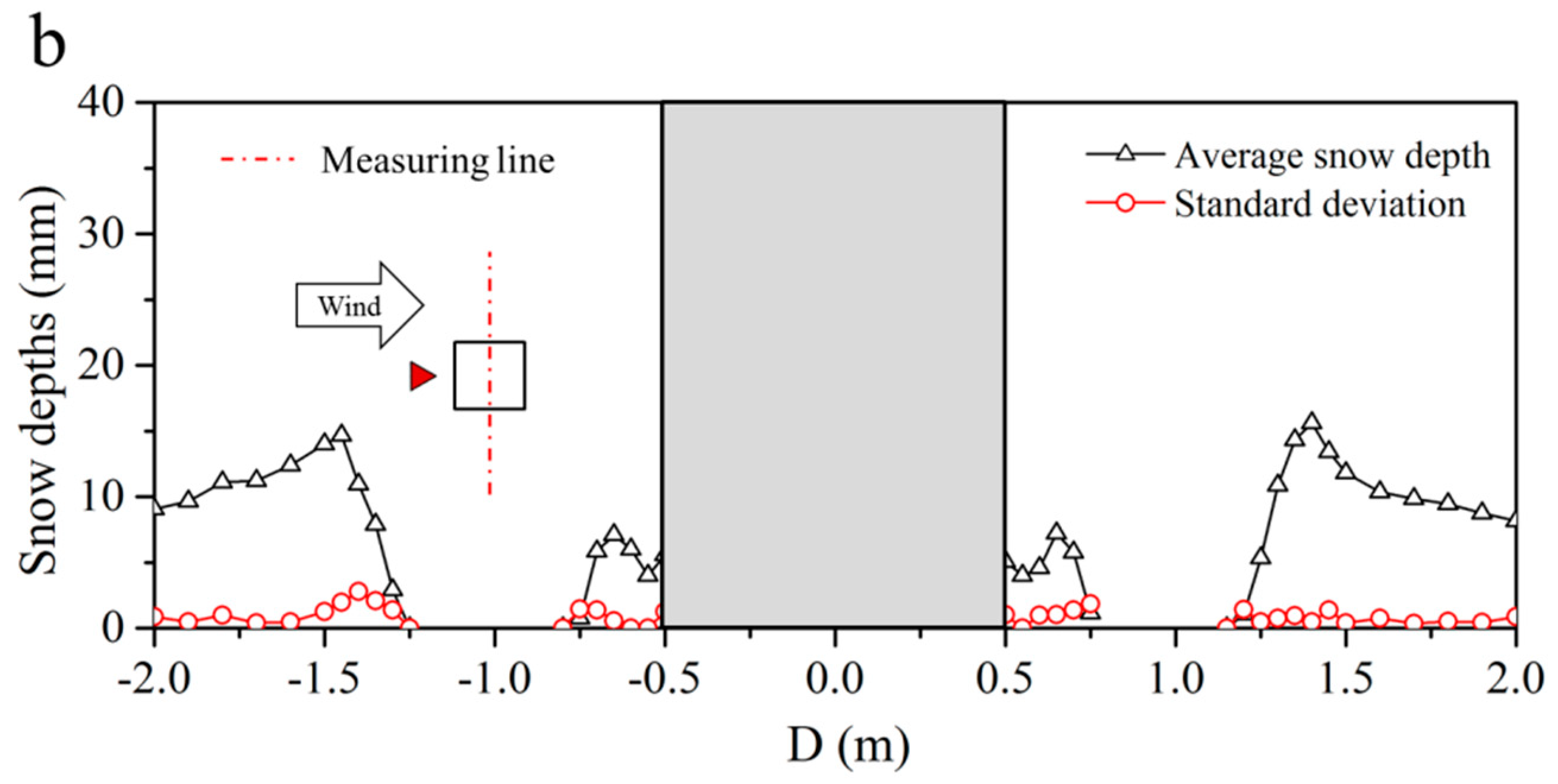
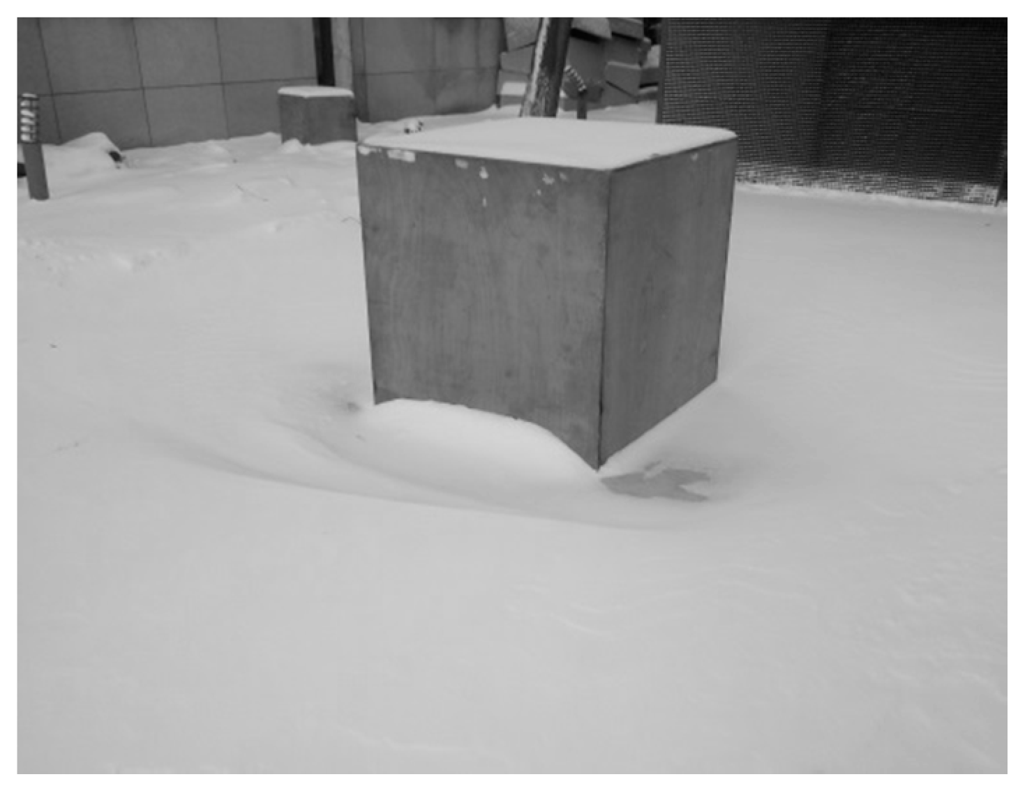
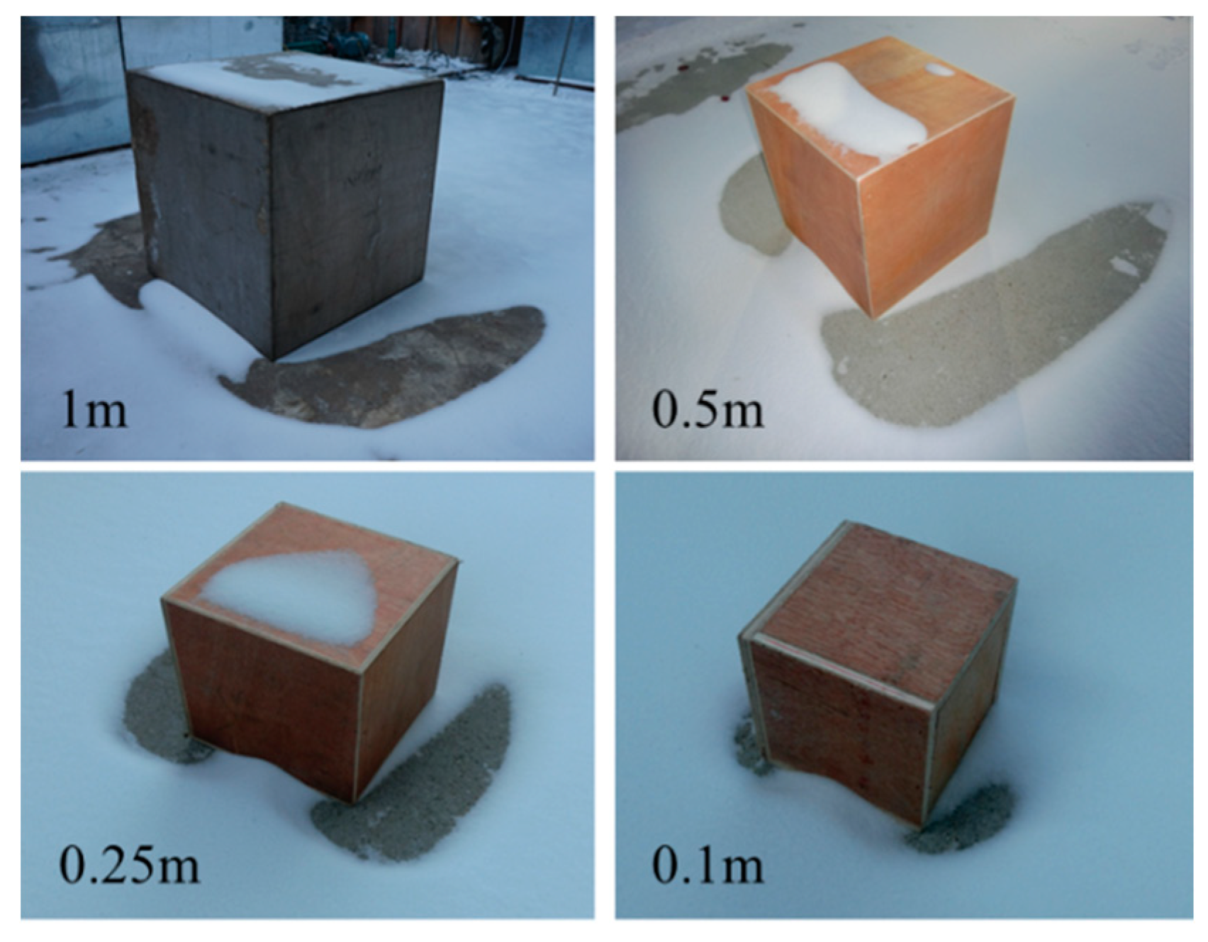
3.4.1. A Field Observation on the 1 m Cube Prototype Model

To confirm the reliability of the new approach, the comparison of field observations and experiments should be done. So, the field observation on a 1 m cube prototype model was conducted on the HIT campus on 11 September 2015 from 0:00 to 6:00. To obtain a reasonably stable wind direction, the test site was located on a narrow strip between two buildings, as shown in Figure 1b. Figure 9 shows the method of observation; the wind field and environment conditions were measured by a PC-4 automatic weather station with a sampling interval of 1 min and the box-type snow flux trapper draws on the design experience summarized by Kimura [31].
The weather station and snow flux instrument were all mounted on the centerline of the model. The wind field during the observation is given in Figure 10. The average snowfall was 29 mm, which was measured on an open and flat ground 20 m away from the model. Figure 11 shows the photo of the snow distribution of the field observation.

3.4.2. Test Similarity Criteria Based on Snowfall Mode

A reliable scale in experimental modeling depends on the right similarity criterion. In order to reproduce the non-uniform snowdrift phenomena caused by structures with scale models, the widely accepted fact is that it is necessary to meet geometric, kinematic, and dynamic similitude requirements.
Since the beginning of snowdrift research,, many different similarity criteria have been proposed, validated, and applied by some famous scholars, such as Strom [32], Odar [33], Calkins [34], Kind [19], Iversen [16], Anno [35], Isyumov [18], Naaim [36], Delpech [21], Beyers [2], and so on.
However, just as it is not possible to satisfy the Froude numbers and Reynolds numbers simultaneously [37], it has been proved that some of the similarity criteria reveal incompatibility, therefore only the most important and widely accepted similarity parameters are selected and discussed.
In the present study, considering the fact that the snow particles falling into the snow bed are provided by the sowing pattern, the experimental modeling is mainly focused on the reliable simulation of the Froude number and drifting volume. The original form of the Froude number is defined as
U 2 g L ,
where U is the reference wind velocity, g is gravitational acceleration (m/s2), and L is the reference length (m). But considering the discrepancy of particle density between the prototype and the test, Odar [33] and Calkins [34] proposed the densimetric Froude number:
ρ ρ p U 2 g L
where ρ is the air density, and ρp is the particle density. To confirm the reliable simulation of drifting volume, Anno [35] suggested that the test should satisfy the following time scaling parameter:
T Q η ρ p L 2
where T is experiment time (s), Q is the transport rate of snow (kg/m·s), and η is the snow collection efficiency. Except for the above similarity, a number of similarity requirements, like the flow field, ejection process, particle trajectory, and deposition pattern, must be satisfied in the experiments on snow drifting on roofs to ensure a reliable simulation.
First, the near ground turbulent wind velocity profile for stable atmospheric conditions is
U = u * κ ln ( z z 0 ) ,
where κ is the Von-Karman constant, u * is the friction velocity, z is the height above the surface, and z0 is the roughness height parameter. Geometric similarity should be enforced through the relationship
D p / L .
Except for the densimetric Froude number expressed as Equation (4), the following Froude number based on the threshold friction velocity should also be satisfied to simulate the shear stress of particles near the ground [16]:
ρ ρ p ρ u * t 2 g D p
where DP is the particle diameter, u * t is the threshold friction velocity, and υ is the kinematic viscosity.
To ensure a similar movement trajectory of a particle, Kind [24] indicated that the following equations must be satisfied:
ρ ρ p ρ u * t 2 g L ,
w f / U ,
where wf is the settling velocity of snow particles (m/s). The deposition or erosion mechanisms could be modeled satisfactorily through the similarity of the particle ejection process [19,38]:
u * / u * t .
In the present study, because the simulation of the Froude number is considered to be more important, the limit of the Reynold number is released. However, to ensure that the inertial forces are dominating the flow, Kind [19] suggested that the following relationship should be satisfied:
u * t 3 2 g v > 30 .
In summary, the parameter (4) and (5) were adopted for determining the wind velocity and experiment time, and several similarity parameters were also chosen for evaluating the results when using a sowing pattern to study snowdrift. In order to verify the reliability of this method, four scale models were selected for the verification test. The experimental conditions are listed in Table 3 and the prototype is the field observation presented above. The reference point for the experimental wind speed was set at 1 m in front of the model along the central line and the height above the ground was equal to the side length of the model. The major similarity parameters for the prototype and scale model are given in Table 4.
Snow flux in the vertical plane was measured by additional experiments with only the snow flux trapper on the testing ground. The snow load coefficient is the ratio of the depth of snow on the roof to the average snowfall. For the experiments, the average snowfall on the ground was determined by an additional experiment conducted for the same duration but without any obstacles in the test section. After the experiments, the snowdrift geometry was measured with the laser total station for about 200~300 points around the model and the measured snow depth data contributed to the contour maps of the snowdrift geometry.

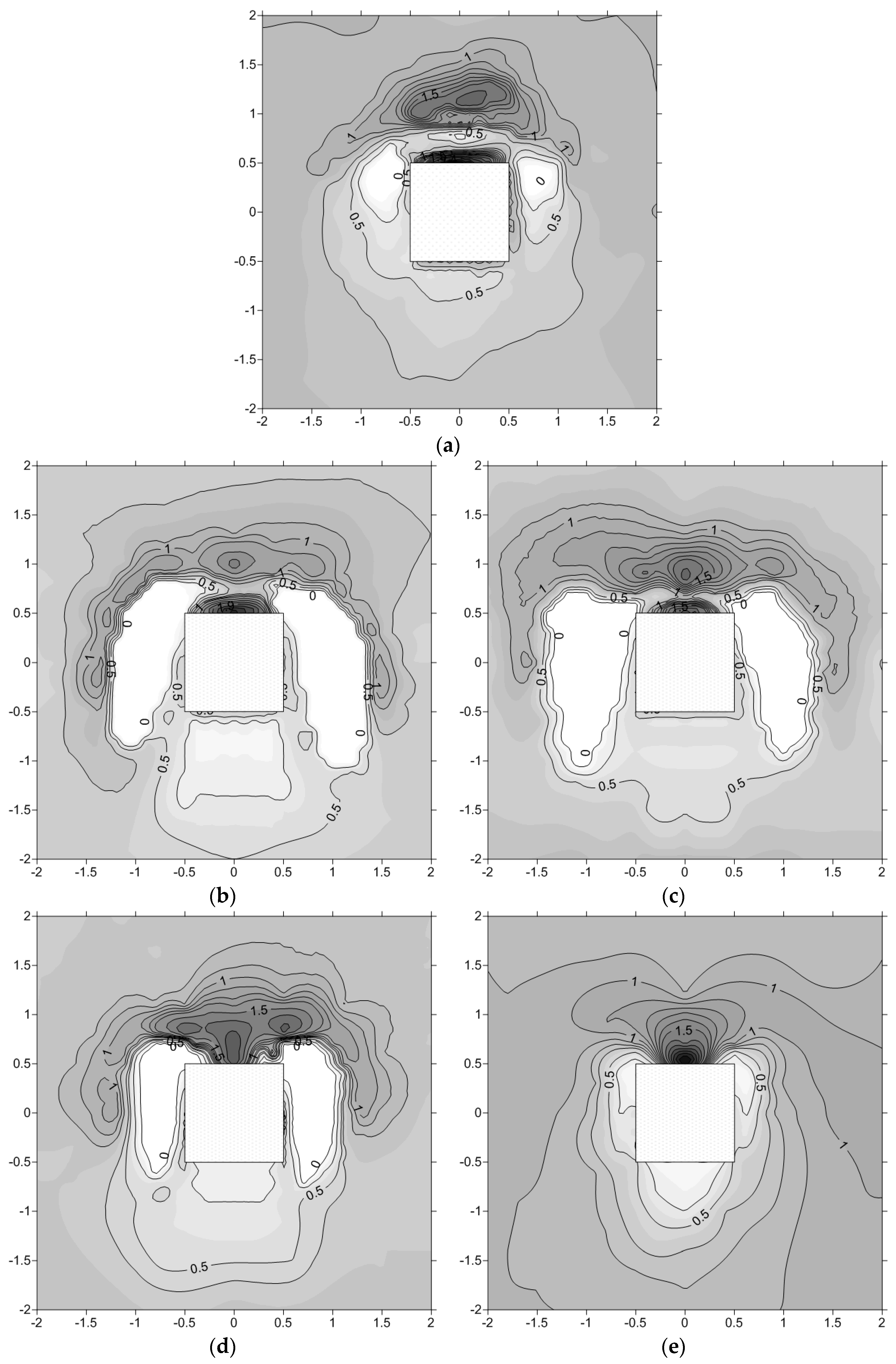
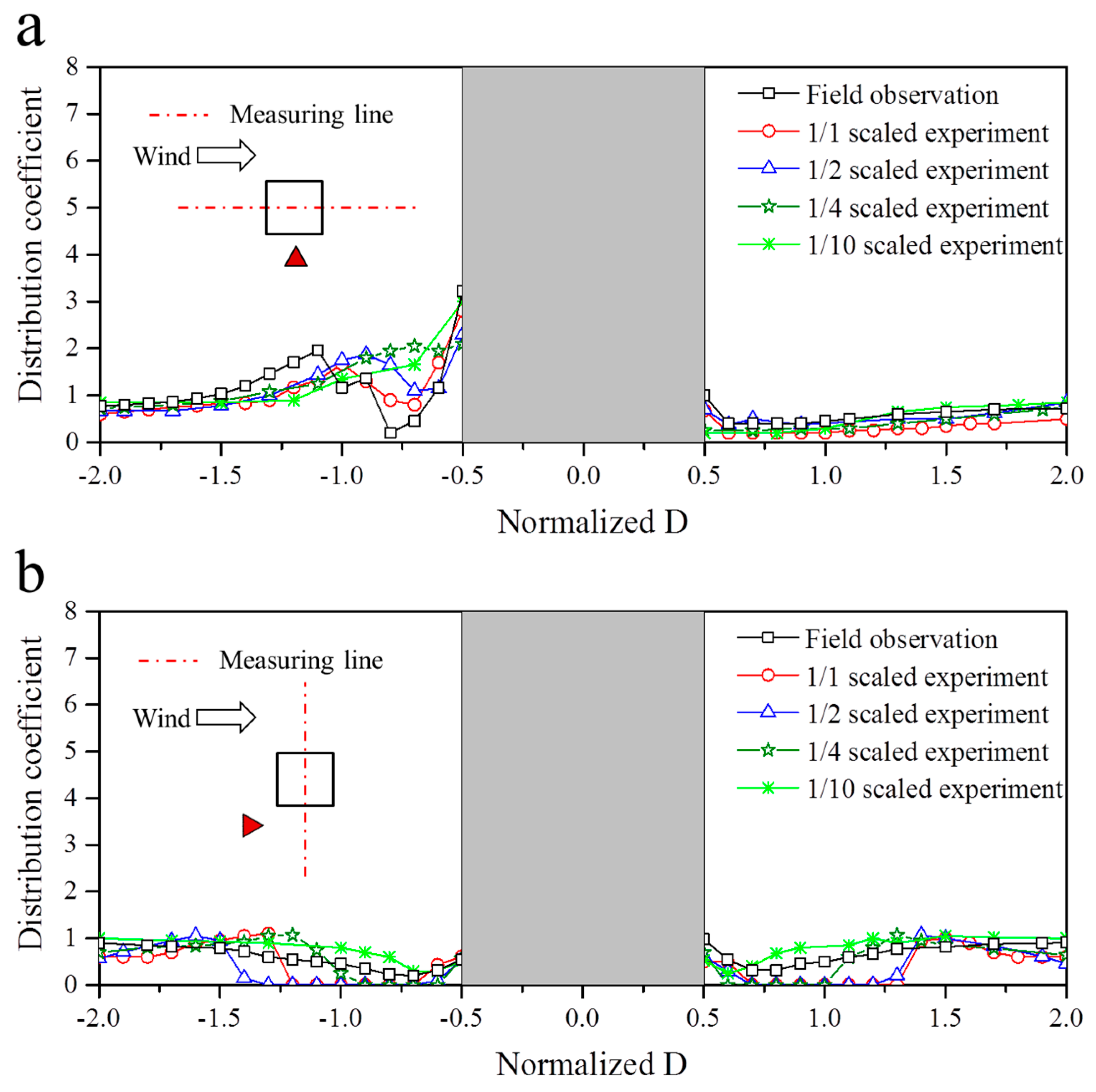
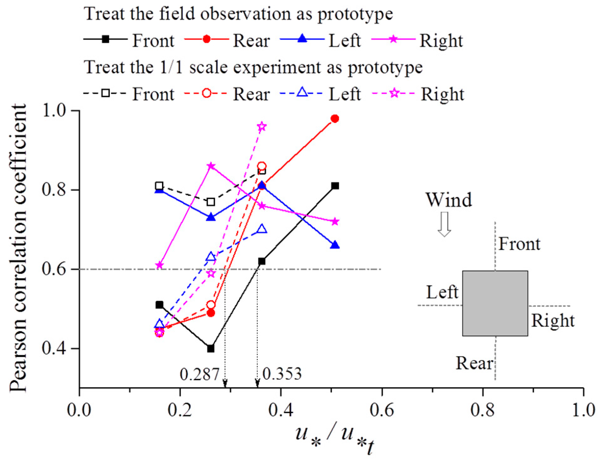
3.4.3. Results and Discussion

There are two key factors to evaluate the accuracy of snowdrift given by the experiments. One is the similarity of the shape of snowdrift; another is the similarity of the snow distribution coefficient. The distribution coefficient is the ratio of measured snow depth and average snowfall at any measuring point.
Figure 12 shows the contour maps of the snowdrift geometry around the model of field observation and scale experiments. The photos of scale experiments are shown in Figure 13. All of the contour maps showed a similar shape which was formed like a horseshoe, in which snow mainly accumulated at the front of the windward side and beginning at the two corners of the windward side, there were two distinct erosion areas near the lateral sides along the downwind direction. From the comparison, if just focusing on the overall distribution shape of the snowdrift, it seemed that the result when the scale was 1/10 was more similar to the field observation and the main erosion areas (near the lateral sides) were larger than field observations for the other scale experiments. The basis for explaining this phenomenon needs an objective and appropriate understanding of the result of the field observation. The main erosion is more distinct in the experiment due to the stable wind speed. However, sometimes there were slight or no wind during the field observation, and snowfall contributes more to decrease the erosion effect in this condition, which would decrease the non-uniform snow distribution to some extent.
However, considering that two distinct snowdrifts were formed in front of the windward side, the results of the 1/1, 1/2, and 1/4 scale experiments had a more similar characteristic of snow distribution. When the scale was 1/10, the snow only accumulated at the feet of the windward side, indicating that wind velocity was excessively reduced; the near to the ground reverse flow in front of the windward side was weak and could not transport snow particles away from the windward side, so that only one distinct snowdrift was formed.
Considering that the effect of fluctuant wind velocity in the field observation could not be ignored, the 1/1 model may be treated as the self-test prototype. In this situation, according to the comparison of results, the 1/2 and 1/4 scale experiment results would have relatively acceptable accuracy of the reproduction of the snowdrift shape of the field observation, but the 1/10 scale experiment result would have a lower precision reproduction.
In order to compare the snow distribution in a more precise method, Figure 14 compares the snow distributions along lateral and streamwise lines crossing the model.
In Figure 14a, it could be seen that the snow distribution of the field observation has obvious characteristics: Near the windward side, the snow formed a compressed “N” shape, and near the leeward side, there formed a compressed “U” shape. When the scale was 1/1 and 1/2, the distribution results showed a good agreement with the field observation, even though the position where the extreme value occurred moved towards to the windward side as the scale ratio decreased. But, as the scale decreased, especially when the scale was 1/10, the snow tended to only accumulate at the foot of the windward side, and the snowdrift away from the windward side disappeared. As for the snow distribution near the leeward side, when the scale was 1/1 and 1/2, the experiments could precisely reproduce the snow distribution, even though the overall value of the coefficient decreased. When the scale was 1/4 and 1/10, the results gave a lower estimate of the snow accumulation, but for the snow distribution away from the leeward side, the results showed better agreement with the field observation both in value and shape.
Snow distribution along the lateral direction is shown in Figure 14b. Except when the scale was 1/10, the snow distribution showed a U-shaped distribution for both field observation and scale experiments. For the 1/10 scale experiment, a similar distribution was found, but the location where the minimum value occurred was much closer to the lateral side. This phenomenon indicates that the erosion effect was excessively decreased.
In summary, considering both the shape of the snowdrift and snow distribution coefficient, except when the scale was 1/10, the results of scale experiments reproduce the field observation accurately, suggesting that the method is reliable.
Especially, it is known that the relationship between friction velocity u * and threshold friction velocity u * t is of great significance in the study of the snowdrift. From the analysis of the similarity parameters in Table 4, it could be derived that a too-small value of the parameter u * / u * t may adversely affect the accuracy of reproduction. Therefore, it is recommended to limit the minimum value of the parameter u * / u * t for scale experiments.
Figure 15 shows the Pearson correlation coefficients of the distribution coefficient between the prototype and scale experiments along the measured line defined as the front, rear, left, and right.
It could be concluded from Figure 15 that the results are of poor quality when the value of the parameter u * / u * t is lower. Assuming that the experiment results are accepted when the Pearson correlation coefficient is higher than 0.6, the lower limit values of the parameter u * / u * t are 0.353 and 0.287, respectively, when the field observation or 1/1 scale experiment is chosen as the prototype. At present, the result of the field observation is affected by the adverse effects of the unstable wind field and the quantitative assessment of the effect is still unclear. So, when giving a suggestion, the analysis based on treating the 1/1 scale experiment as a prototype should be more respected and, finally, 0.3 is suggested to be the lower limit value of parameter u * / u * t in the present study.

4. Conclusions

In the present study, a new approach based on a snow–wind combined experiment facility, for investigating snow distribution, is introduced, including its concept, design, operation, and verification.
According to the above work, the following conclusions could be drawn:
(1)
According to 20 repetitive experiments, the results show high correspondence with each other and this indicates that the experimental conditions provided by the new experiment facility are stable. From the comparison between field observation and scale experiments, it proves that the proposed experimental approach and adopted similitude criteria are reliable. The two pieces of evidence indicate that the new approach is credible and feasible.
(2)
The comparison of results from field observations and scale experiments indicate that when the wind velocity is excessively reduced, the result is not satisfactory. The lower limit value of the parameter u * / u * t is suggested for ensuring the accuracy of the reproduction. In the present study, taking into consideration the instability of field observations objectively and combining with the results of scale experiments, 0.3 is suggested to be the lower limit value of parameter u * / u * t .
In this paper, only experiments on snowdrift around a cube were chosen for the verification for the sake of generality, but this method could also be adopted for the prediction of snowdrift around complex building environments and snow loads on various shapes of building roofs. It could provide a basis for site selection planning for buildings and the safety design of roof structures in snowy areas.

Author Contributions

Conceptualization, Q.Z.; data curation, M.L.; formal analysis, M.L. and Q.Z.; funding acquisition, F.F.; investigation, M.L.; methodology, M.L. and Q.Z.; project administration, F.F.; resources, F.F.; software, M.L.; supervision, Q.Z. and S.S.; validation, M.L., Q.Z., F.F. and S.S.; visualization, Q.Z.; writing—original draft, M.L.; writing—review and editing, Q.Z.

Funding

This research was funded by the National Natural Science Foundation of China, grant number 51508133, 51478147, and the National Outstanding Youth Science Fund Project of the National Natural Science Foundation of China, grant number 51525802.

Acknowledgments

This work was financially supported by the National Natural Science Foundation of China (Grant no. 51508133, 51478147), the National Outstanding Youth Science Fund Project of National Natural Science Foundation of China (51525802), and Foundation of Key Laboratory of Structures Dynamic Behavior and Control (Ministry of Education) in Harbin Institute of Technology (HITCE201704). The authors are grateful to the members of the Space Structures Research Center in Harbin Institute of Technology, for providing invaluable information and advice in this study.

Conflicts of Interest

The authors declare no conflict of interest.

References

  1. Thomas, K. This Large scale studies of development of snowdrifts around buildings. J. Wind Eng. Ind. Aerodyn. 2003, 91, 829–839. [Google Scholar]
  2. Beyers, J.H.M.; Harms, T.M. Outdoors modelling of snowdrift at SANAE IV Research Station, Antarctica. J. Wind Eng. Ind. Aerodyn. 2003, 91, 551–569. [Google Scholar] [CrossRef]
  3. Thomas, K.; Thiis, Y.G. Large-scale measurements of snowdrifts around flat-roofed and single-pitch-roofed buildings. Cold Reg. Sci. Technol. 1999, 30, 175–181. [Google Scholar]
  4. Beyers, J.H.M.; Sundsb, P.A.; Harms, T.M. Numerical simulation of three-dimensional, transient snow drifting around a cube. J. Wind Eng. Ind. Aerodyn. 2004, 92, 725–747. [Google Scholar] [CrossRef]
  5. Høibø, H. Snow Load on Gable Roofs—Results from Snow Load Measurements on Farm Buildings in Norway. In Proceedings of the First International Conference on Snow Engineering, Santa Barbara, CA, USA, 1988; pp. 95–104, Special Report 89–6. [Google Scholar]
  6. Høibø, H. Form factors for snow load on gable roofs -Extending use of snow load data from inland districts to wind-exposed areas. In Proceedings of the 11th International Congress on Agricultural Engineering, Dublin, Ireland, 4–8 September 1989. [Google Scholar]
  7. Uematsu, T.; Nakata, T.; Takeuchi, K. Three-dimensional numerical simulation of snowdrift. Cold Reg. Sci. Technol. 1991, 1, 65–73. [Google Scholar] [CrossRef]
  8. Tominaga, Y.; Mochida, A. CFD prediction of flowfield and snowdrift around a building complex in a snowy region. J. Wind Eng. Ind. Aerodyn. 1999, 81, 273–282. [Google Scholar] [CrossRef]
  9. Beyers, M.; Waechter, B. Modeling transient snowdrift development around complex three-dimensional structures. J. Wind Eng. Ind. Aerodyn. 2008, 96, 1603–1615. [Google Scholar] [CrossRef]
  10. Tominaga, Y.; Okaze, T.; Mochida, A. CFD modeling of snowdrift around a building: An overview of models and evaluation of a new approach. Build. Environ. 2011, 46, 899–910. [Google Scholar] [CrossRef]
  11. Okaze, T.; Takano, Y.; Mochida, A.; Tominaga, Y. Development of a new k–ε model to reproduce the aerodynamic effects of snow particles on a flow field. J. Wind Eng. Ind. Aerodyn. 2015, 144, 118–124. [Google Scholar] [CrossRef]
  12. Liston, G.E.; Haehnel, R.B.; Sturm, M.; Hiemstra, C.A.; Berezovskaya, S.; Tabler, R.D. Simulating complex snow distributions in windy environments using SnowTran-3D. Glaciology 2007, 53, 241–256. [Google Scholar] [CrossRef] [Green Version]
  13. Tominaga, Y. Numerical simulation of snowdrift around buildings: Past achievements and future perspectives. In Proceedings of the Snow Engineering VIII, Nante, France, 14–17 June 2016. [Google Scholar]
  14. Thiis, T.K.; Ramberg, J.F. Measurements and numerical simulations of development of snowdrifts of curved roofs. In Proceedings of the Snow Engineering VI, Whistler, CO, Canada, 1–5 June 2008. [Google Scholar]
  15. Thiis, T.K.; Potac, J.; Ramberg, J.F. 3D numerical simulations and full scale measurements of snow depositions on a curved roof. In Proceedings of the 5th European & African Conference on Wind Engineering, Florence, Italy, 19–23 July 2009. [Google Scholar]
  16. Iversen, J.D. Comparison of wind-tunnel model and full-scale snow fence drifts. J. Wind Eng. Ind. Aerodyn. 1981, 8, 231–249. [Google Scholar] [CrossRef]
  17. Sant’Anna, F.D.M.; Taylor, D.A. Snow drifts on flat roofs: Wind tunnel tests and field measurements. J. Wind Eng. Ind. Aerodyn. 1990, 34, 223–250. [Google Scholar] [Green Version]
  18. Isyumov, N.; Mikitiuk, M. Wind tunnel model tests of snow drifting on a two level flat roof. J. Wind Eng. Ind. Aerodyn. 1990, 36, 893–904. [Google Scholar] [CrossRef]
  19. Kind, R.J. A Critical examination of the requirements for model simulation of wind-induced erosion/deposition phenomena such as snow drifting. Atmos. Environ. 1976, 10, 219–227. [Google Scholar] [CrossRef]
  20. Kind, R.J. A Review of Modelling Methods. Cold Reg. Sci. Technol. 1986, 12, 217–228. [Google Scholar] [CrossRef]
  21. Delpech, P.H.; Palier, P.; Gandemer, J. Snowdrifting Simulation around Antarctic Buildings. J. Wind Eng. Ind. Aerodyn. 1998, 74–76, 567–576. [Google Scholar] [CrossRef]
  22. Okaze, T.; Mochida, A.; Tominaga, Y. Wind tunnel investigation of drifting snow development in a boundary layer. J. Wind Eng. Ind. Aerodyn. 2012, 104–106, 532–539. [Google Scholar] [CrossRef]
  23. Hui, L.; Huang, N.; Tong, D. Wind tunnel experiments on natural snow drift. Sci. China Technol. Sci. 2012, 55, 927–938. [Google Scholar]
  24. Zhou, X.; Hu, J.; Gu, M. Wind tunnel test of snow loads on a stepped flat roof using different granular materials. Nat. Hazards 2014, 74, 1629–1648. [Google Scholar] [CrossRef]
  25. Zhou, X.; Kang, L.; Yuan, X.; Gu, M. Wind tunnel test of snow redistribution on flat roofs. Cold Reg. Sci. Technol. 2016, 127, 49–56. [Google Scholar] [CrossRef]
  26. Delpech, P.H.; Thomas, K.T. Applications of snowind engineering-climatic wind tunnel methods, Technical transaction iss.12. Civil Eng. 2015, 2-B, 381–403. [Google Scholar]
  27. Oikawa, S.; Tomabechi, T.; Ishihara, T. One-day Observations of Snowdrifts Around a Model Cube. J. Snow Eng. Jpn. 1999, 15, 283–291. [Google Scholar] [CrossRef]
  28. Liu, M.; Zhang, Q.; Fan, F.; Shen, S. Experiments on natural snow distribution around simplified building models based on open air snow-wind combined experiment facility. J. Wind Eng. Ind. Aerodyn. Shizhao 2018, 1–13, 173. [Google Scholar] [CrossRef]
  29. Pietersma, D.; Stetler, L.D.; Saxton, K.E. Design and aerodynamies of a Portable wind tunnel for soil erosion and fugitive dust researeh. Trans. ASAE 1996, 39, 2075–2083. [Google Scholar] [CrossRef]
  30. Tominaga, Y.; Okaze, T.; Mochida, A.; Shida, T.; Yoshino, H. CFD prediction of snowdrift around a cubic building model. In Proceedings of the Snow Engineering VI, Whistler, CO, Canada, 1–5 June 2008. [Google Scholar]
  31. Kimura, T. Measurements of Drifting Snow Particles. J. Geogr. 1991, 100, 250–263. [Google Scholar] [CrossRef]
  32. Strom, G.H.; Kelly, G.R.; Deitz, E.L.; Weiss, R.F. Scale Model Studies on Snow Drifting; Research Report 73; U.S. Army Snow, Ice and Permafrost Research Establishment: Hanover, NH, USA, 1962. [Google Scholar]
  33. Odar, F. Simulation of Drifting Snow; Research Report 174; Cold Regions Research and Engineering Laboratory: Hanover, NH, USA, 1965. [Google Scholar]
  34. Calkins, D.J. Model Studies of Drifting Snow Patterns at Safeguard Facilities in North Dakota, United States Army, Corps of Engineer; Cold Regions Research & Engineering Laboratory: Hanover, NH, USA, 1974; 20p. [Google Scholar]
  35. Anno, Y. Requirements for modeling of a snowdrift. Cold Reg. Sci. Technol. 1984, 8, 241–252. [Google Scholar] [CrossRef]
  36. Naaim-Bouvet, F. Comparison of requirements for modeling snowdrift in the case of outdoor and wind tunnel experiments. Surv. Geophys. 1995, 16, 711–727. [Google Scholar] [CrossRef]
  37. White, F.M. Viscous Fluid Flow; McGraw-Hill: New York, NY, USA, 1991. [Google Scholar]
  38. Kind, R.J.; Murray, S.B. Saltation flow measurements relating to modeling of snowdrifting. J. Wind Eng. Ind. Aerodyn. 1982, 10, 89–102. [Google Scholar] [CrossRef]
Figure 1. (a) Photo of the snow–wind combined experiment facility. (b) Location of the facility.
Applsci 09 03393 g001
Figure 2. Schematic view of the snow–wind combined experiment facility.
Applsci 09 03393 g002
Figure 3. A sketch of the experimental procedure.
Applsci 09 03393 g003
Figure 4. A sketch of the measuring method.
Applsci 09 03393 g004
Figure 5. Wind field on the first line of the five sections: (a) mean wind and (b) turbulence intensity.
Applsci 09 03393 g005
Figure 6. Wind field on the section which is 4 m away from the outlet: (a) mean wind and (b) turbulence intensity.
Applsci 09 03393 g006
Figure 7. Some photos of the repetitive experiments.
Applsci 09 03393 g007
Figure 8. Results of the 20 experiments: (a) streamwise direction (center section) and (b) lateral section (center section).
Applsci 09 03393 g008aApplsci 09 03393 g008b
Figure 9. Abridged general view of field observation.
Applsci 09 03393 g009
Figure 10. Wind field during the observation.
Applsci 09 03393 g010
Figure 11. Photo of snow distribution for the field observation.
Applsci 09 03393 g011
Figure 12. Contour maps of the snowdrift geometry around the model: (a) field observation; (b) experiment with a 1 m Cube model; (c) experiment with a 0.5 m Cube model; (d) experiment with a 0.25 m Cube model; and (e) experiment with a 0.1 m Cube model.
Applsci 09 03393 g012
Figure 13. Photos of scale experiments.
Applsci 09 03393 g013
Figure 14. Comparison between normalized snow depths obtained from field observations and scale experiments: (a) streamwise direction (center section) and (b) lateral direction (center section).
Applsci 09 03393 g014
Figure 15. Pearson correlation coefficients of the distribution coefficient between the prototype and scale experiments.
Applsci 09 03393 g015
Table 1. Comparison of the physical parameters of the snow particles.
ReferenceDensity (kg/m3)Terminal Velocity (m/s)Diameter (mm)Angle of Repose (°)
Field observation of fresh snow in this paper100~1500.300.15~1.065
Stored snow in this paper220~3100.500.2~0.555
Thiis and Ramberg [14]500.500.20
Tominaga and Okaze [30]1500.200.15
Oikawa and Tomabechi [27]50~1500.200.1560
Table 2. Environmental conditions of the 20 repetitive experiments.
Experiment Wind SpeedTemperatureHumidityMax Natural WindBulk Density of SnowTesting Time
2.5 m/s0 °C78%0.13 m/s250.6 kg/m31 h
2.5 m/s0 °C78%0.30 m/s260.2 kg/m31 h
2.5 m/s−1 °C76%0.28 m/s255.8 kg/m31 h
2.5 m/s−1 °C76%0.19 m/s236.7 kg/m31 h
2.5 m/s−1 °C76%0.22 m/s227.5 kg/m31 h
2.5 m/s−1 °C76%0.23 m/s240.4 kg/m31 h
2.5 m/s−2 °C74%0.18 m/s266.6 kg/m31 h
2.5 m/s−2 °C73%0.15 m/s270.1 kg/m31 h
2.5 m/s−2 °C73%0.22 m/s252.4 kg/m31 h
2.5 m/s−2 °C68%0.14 m/s261.9 kg/m31 h
2.5 m/s−2 °C68%0.20 m/s242.3 kg/m31 h
2.5 m/s−2 °C67%0.30 m/s248.6 kg/m31 h
2.5 m/s−2 °C68%0.17 m/s233.6 kg/m31 h
2.5 m/s−2 °C66%0.19 m/s239.5 kg/m31 h
2.5 m/s−3 °C64%0.16 m/s257.4 kg/m31 h
2.5 m/s−3 °C63%0.11 m/s244.5 kg/m31 h
2.5 m/s−3 °C63%0.21 m/s221.0 kg/m31 h
2.5 m/s−3 °C61%0.15 m/s235.2 kg/m31 h
2.5 m/s−3 °C60%0.12 m/s243.3 kg/m31 h
2.5 m/s−3 °C60%0.12 m/s266.4 kg/m31 h
Table 3. Environmental conditions of the scale experiments.
Model ScaleVelocity (m/s)Snow Mass Flux (kg/m2·s)Experiment Time (min)
Prototype2.4751.93 × 10−3360
13.52.81 × 10−250
0.52.51.52 × 10−246
0.251.88.49 × 10−341
0.11.13.68 × 10−338
Table 4. Similarity parameters of prototype and scale models.
Similarity ParametersPrototype10.50.250.1
D p / L 0.0020.0030.0060.0120.03
ρ ρ p ρ u * t 2 g D p 0.01160.01540.01540.01540.0154
ρ ρ p ρ u * t 2 g L 2.32 × 10−54.61 × 10−59.23 × 10−51.85 × 10−44.61 × 10⁻⁴
w f / U 0.1210.1430.2000.2780.455
u * / u * t 0.7170.5070.3620.2610.159
u * t 3 2 g v > 30 -99.9299.9299.9299.92

