Exploring Efficient Neural Architectures for Linguistic–Acoustic Mapping in Text-To-Speech ^†

Abstract

Conversion from text to speech relies on the accurate mapping from linguistic to acoustic symbol sequences, for which current practice employs recurrent statistical models such as recurrent neural networks. Despite the good performance of such models (in terms of low distortion in the generated speech), their recursive structure with intermediate affine transformations tends to make them slow to train and to sample from. In this work, we explore two different mechanisms that enhance the operational efficiency of recurrent neural networks, and study their performance–speed trade-off. The first mechanism is based on the quasi-recurrent neural network, where expensive affine transformations are removed from temporal connections and placed only on feed-forward computational directions. The second mechanism includes a module based on the transformer decoder network, designed without recurrent connections but emulating them with attention and positioning codes. Our results show that the proposed decoder networks are competitive in terms of distortion when compared to a recurrent baseline, whilst being significantly faster in terms of CPU and GPU inference time. The best performing model is the one based on the quasi-recurrent mechanism, reaching the same level of naturalness as the recurrent neural network based model with a speedup of 11.2 on CPU and 3.3 on GPU.

1. Introduction

Speech synthesis is the computerized generation of speech. In text-to-speech (TTS), speech generation is conditioned on written linguistic contents [1]. Current TTS systems use statistical models such as deep neural networks to map linguistic and prosodic features extracted from a text processing front-end to some acoustic representation. This acoustic representation can either be the waveform itself, such as the one generated by WaveNet [2], WaveRNN [3], or SampleRNN [4], or acoustic features extracted after a vocoding process [5]. The latter are known to be more efficient to generate speech, despite being less natural in terms of voice quality.

Apart from the acoustic representation used as output, another distinction in current TTS statistical models is whether they use a two-stage linguistic–acoustic mapping or work in an end-to-end manner. On the one hand, mapping models work by first predicting the number of frames (duration) of a phoneme with a duration model, and then predicting the frames themselves out of the linguistic contents and the predicted duration with the acoustic model [6,7,8]. On the other hand, end-to-end models directly predict the acoustic signal from the linguistic contents without an intermediate duration prediction step. This is done through the so-called attention mechanism, which is a learnable alignment model embedded between the linguistic encoder and the acoustic decoder that adapts the sequential resolution difference from input to output. Many end-to-end models have recently been proposed with the availability of large amounts of speech and text data, as well as powerful computational resources to train them. Examples of these models are Tacotron [9,10,11], DeepVoice [12,13,14,15], Char2Wav [16], or Transformer TTS [17].

We focus our analysis on the linguistic–acoustic mapping within two-stage TTS systems, which tends to require fewer data and resources to be trained than end-to-end systems. Additionally, we can decouple the actual effects of acoustic modeling from the linguistic alignment in this way, so that we see more clearly the effects of changing only the inner structure of the acoustic decoder. Different works used this design, outperforming previously existing statistical parametric speech synthesis systems, which used to rely on hidden Markov models. This was done with different variants of prosodic and linguistic features, as well as perceptual losses of different kinds in the acoustic mapping [18,19,20,21,22]. Since speech synthesis is a sequence generation problem, models that capture temporal dynamics are a natural fit to this task. Recurrent neural networks (RNNs) are a specific neural topology with feedback connections that allow modeling a memory component, which tracks activations in time in addition to the classic feed-forward path from input to output. They have thus been used as deep architectures that effectively predict either prosodic features [23,24], or duration and acoustic features [7,25,26,27]. Some of these works also investigate possible performance differences using different RNN cell types, such as long short-term memory (LSTM) or gated recurrent unit modules [28].

Despite the success of RNNs in the sequential modeling paradigm, recent investigations proved the effectiveness of other mechanisms that rely on structures different from the classic recurrent ones. Other recurrent-like variants were proposed to overcome the computation burden that projected recurrent connections impose. For instance, the quasi-RNN (QRNN) moves these projections to a feed forward case while maintaining a memory vector that gets updated with element-wise interactions [29]. Hence, QRNNs may be used as a replacement for LSTMs. Their effectiveness in different natural language processing (NLP) tasks compared to LSTMs has been proven [29,30], with empirical evidence showing they can speed up sequence processing by 16 times with respect to LSTMs. They have also been used in end-to-end TTS systems, such as the aforementioned DeepVoice [12], as conditioning to processors to upsample linguistic and prosodic features to the waveform resolution used by a WaveNet generator. Another system is the Transformer network, which also conceptualizes sequential dependencies differently from RNNs, avoiding any sort of recurrent connection. The Transformer network was designed as a sequence-to-sequence model for machine translation, where typically RNNs are applied to deal with the conversion between the two sequences [31,32]. In [33], Vaswani et al. specifically introduced the self-attention mechanism, which can relate elements within a single sequence regardless of the sequential order by using a compatibility function. Nonetheless, the order awareness is important, thus, in this system, it is imposed with positioning codes that serve as time-stamps (so input features rather than neural connections).

In this article, which continues from our previous work [34], we investigate the performance in terms of both prediction efficiency and voice quality of three types of sequential processing architectures for linguistic–acoustic mapping in two-stage TTS systems. Firstly, we depart from an RNN reference model that uses LSTM cells, as proposed in previous works [7,8]. Secondly, we use a QRNN-based model named QRNN linguistic–acoustic decoder (QLAD), based on the previous mentioned evidence of more efficient computations than LSTM structures, albeit being comparable in performance across different sequential tasks. QRNNs have been used in the conditioning branch of end-to-end TTS, as mentioned above, but we instead propose them to actually generate the acoustic parameter trajectories of our decoder. We also consider a Transformer encoder, thus discarding its original attention decoder structure, because we are dealing with a mapping between two sequences that have the same time resolution. We however call this part the decoder in our case, given that we are decoding linguistic contents into their acoustic codes. Precisely a key difference between our Transformer module and the recently proposed Transformer TTS is that we do not work with the full Transformer structure as other end-to-end solutions do [17]. We thus call this system the self-attention linguistic acoustic–decoder (SALAD) [34]. Acoustic models that improve the speech synthesis efficiency over the existing RNN-based ones are a suitable target for low resource environments as long as the generated speech quality is not degraded. This specially fits embedded devices, such as mobile phones, with which the TTS system can then run locally. Furthermore, the experimentation carried out in this work is applicable to further settings where text is not the input signal but speech is the synthesized output (e.g., speech enhancement or voice conversion [35,36], where speech signals are converted into other speech signals). Moreover, some of these architectural changes can also be extended for more end-to-end waveform generation solutions similar to those of WaveNet [2] or WaveRNN [3]. Nonetheless, our focus is on exploring these variations on the vocoder acoustic parameter generation for ease of experimentation, both in computational requirements and given the amount of training data available to succeed in the level of synthesized naturalness.

We empirically found that both QLAD and SALAD models are competitive in terms of efficiency for training and inference. Additionally, both models show competitive objective results against those of the RNN. Nonetheless, QLAD models are the only ones that subjectively match, or even improve in some setting, the voice naturalness of RNNs.

This paper is structured as follows. In Section 2, we introduce the linguistic–acoustic decoding framework we worked with, based on an RNN acoustic model. We then describe the QLAD and SALAD models in Section 3 and Section 4. Then, in Section 5, we describe the followed experimental setup, specifying the data, the features, and the hyper-parameters chosen for the overall architectures. Finally, results and conclusions are shown and discussed in Section 6 and Section 7, respectively. The code for the proposed model and the baselines can be found in our public repository (https://github.com/santi-pdp/musa_tts).

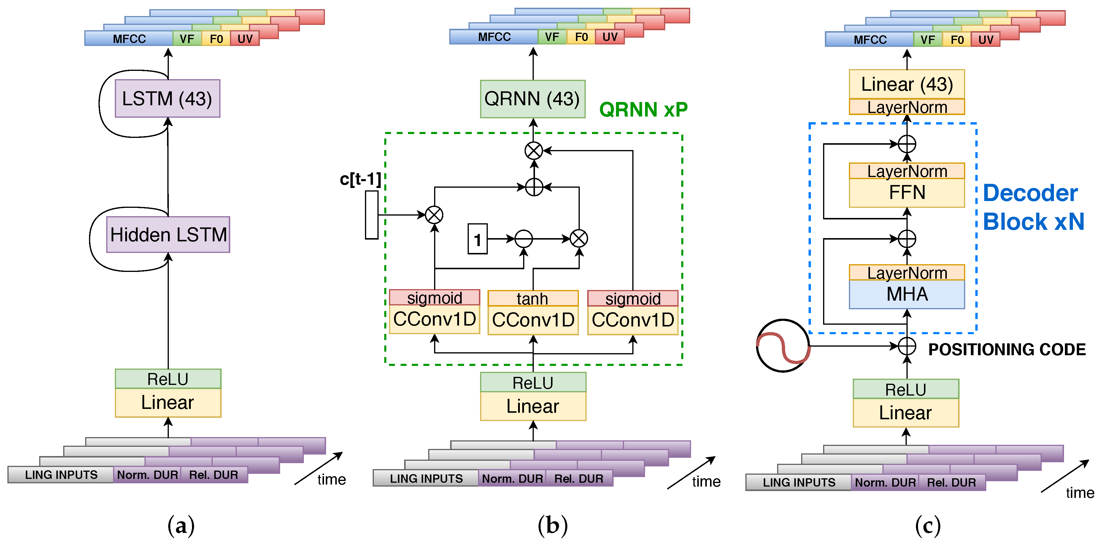
2. Recurrent Neural Network Based Linguistic–Acoustic Decoder

To study the introduction of our proposed networks into a TTS system, we employed our previous multiple speaker adaptation (MUSA) framework [8,27,37]. This is a two-stage RNN model influenced by the work of Zen and Sak [7], in the sense that it uses unidirectional LSTMs to build the duration model and the acoustic model without the need of predicting dynamic acoustic features. A key difference between our works and that of Zen and Sak is the capacity to model many speakers and adapt the acoustic mapping among them with different output branches, as well as interpolating new voices out of a common representation. Nonetheless, for the current work, we did not use this multiple speaker capability and focused on just single speaker models (one model per speaker) for the new architecture design on improving the acoustic model. This way we can decouple architectural effects from shared representations, training each speaker model with a comparable amount of data and the same number of parameters.

Figure 1 depicts the linguistic–acoustic decoder of MUSA across the different structures explored in this work. The input to the model is a sequence of frames, each one containing a mixture of linguistic and duration features). Then, each structure outputs a frame of 43 acoustic parameters per time-step. Both linguistic and acoustic features used in this work are detailed in Section 5.2. The MUSA framework with RNNs is shown in Figure 1a. As a first step, we have a pre-projection, fully-connected layer with a ReLU activation. This embeds the mixture ${\mathbf{x}}_t$ of different input types into a common dense representation ${\mathbf{h}}_t$ in the form of one vector per time step t. Hence, the transformation ${\mathbb{R}}^L\to {\mathbb{R}}^H$ is applied independently at each time step t as

$${\mathbf{h}}_t=max(0,\mathbf{W}{\mathbf{x}}_t+\mathbf{b}),$$

(1)

where $\mathbf{W}\in {\mathbb{R}}^{H\times L}$, $\mathbf{b}\in {\mathbb{R}}^H$, ${\mathbf{x}}_t\in {\mathbb{R}}^L$, and ${\mathbf{h}}_t\in {\mathbb{R}}^H$. After this projection, we have the recurrent core formed by an LSTM layer of H cells and an additional LSTM output layer. The output is recurrent, as this prompted better results than using dynamic features to smooth cepstral trajectories in time when using RNNs [7].

3. QRNN Linguistic–Acoustic Decoder

The QRNN was proposed as an efficient alternative to classic RNN cells, such as LSTMs, by removing the affine projections from recurrent connections. The equation that drives classic RNNs is

$${\mathit{h}}_t=tanh(\mathit{W}{\mathit{x}}_t+\mathit{U}{\mathit{h}}_{t-1}+\mathit{b})$$

(2)

where matrix $\mathit{U}\in {\mathbb{R}}^H$ is used to project each previous time-step state ${\mathit{h}}_{t-1}$ and to mix these features with current new inputs ${\mathit{x}}_t$, thus obtaining the current state ${\mathit{h}}_t$. This temporal dependency with $\mathit{U}$ connections dramatically limit parallelism and make RNNs unwieldy for very long sequences, where $\mathit{U}$ matrix projects up to T times each ${\mathit{h}}_t$, being T the total sequence duration. In contrast to this, QRNNs alternate convolutional layers, applied in parallel across timesteps, with minimalist recurrent pooling functions that apply in parallel across channels. Despite having no trainable recurrent connections (i.e., removing $\mathit{U}$), QRNNs proved to be very effective in different NLP tasks, in comparison to their LSTM counterpart, when enough QRNN layers are stacked [29].

The first QRNN stage operates with a series of convolutional blocks, which can process all input time-steps in parallel. As we apply the QRNN after the embedding layer introduced in Section 2, we have the tensor $\mathbf{X}=[{\mathbf{h}}_1,\cdots ,{\mathbf{h}}_T]\in {\mathbb{R}}^{T\times H}$ containing the embeddings at all time-steps. We formulate the convolutional projections as

$$\begin{array}{l}\mathbf{Z}=tanh({\mathbf{W}}_z\ast \mathbf{X})\\ \mathbf{F}=\sigma ({\mathbf{W}}_f\ast \mathbf{X})\\ \mathbf{O}=\sigma ({\mathbf{W}}_o\ast \mathbf{X}),\end{array}$$

(3)

where ${\mathbf{W}}_z$, ${\mathbf{W}}_f$ and ${\mathbf{W}}_o$ are convolutional filter banks that predict the cell activation, the forget gate activation, and the output gate activation, respectively. The sizes of these filter banks are ${\mathbb{R}}^{K\times H\times M}$, being K each kernel width, H the number of input channels, and M the number of convolutional kernels. Note that $\mathbf{Z}$, $\mathbf{F}$, and $\mathbf{O}$ are of dimension $T\times M$, thus all T time-steps are processed in parallel by each filter bank. After obtaining these activations, we can pass them to the aforementioned recurrent pooling, defined as

$$\begin{array}{c}{\mathbf{c}}_t={\mathbf{f}}_t\odot {\mathbf{c}}_{\mathbf{t}-\mathbf{1}}+(1-{\mathbf{f}}_t)\odot {\mathbf{z}}_t\hfill \\ {\mathbf{h}}_t={\mathbf{o}}_t\odot {\mathbf{c}}_t,\hfill \end{array}$$

(4)

where ⊙ denotes element-wise multiplication. Note that each vector, indexed by t, is a time-slice of each of the previously defined activation tensors $\mathbf{Z}$, $\mathbf{F}$, and $\mathbf{O}$. These operations are similar to the ones defined in RNNs, but note how we have no affine transformation between time-steps in this case. Hence, the key to QRNN efficiency is that all learnable parameters are conveyed in the parallel computation phase. The described operations are depicted in Figure 1b. The QRNN layer is contained within the green dashed line, and we stack up to P different layers. Finally, the output QRNN, analogous to the RNN version, is also stacked. This architecture can thus be seen as an intermediate step between full recurrence and no recurrence at all, and we name it QLAD.

4. Self-Attention Linguistic–Acoustic Decoder

Based on the Transformer architecture [33], we also consider a pseudo-sequential processing network that can leverage distant element interactions within the input linguistic sequence to predict acoustic features [34]. This is similar to what an RNN does, but discarding any recurrent connection. This allows us to process all input elements in parallel at inference, hence substantially accelerating the acoustic predictions. In our setup, we do not face a sequence-to-sequence problem as stated previously, so we only use a structure similar to the Transformer encoder, which we call a linguistic–acoustic decoder.

The SALAD architecture begins with the same embeddings of linguistic and prosodic features from Section 2, followed by a positioning encoding system. As we have no recurrent structure, and hence no processing order, this positioning encoding system allows the upper parts of the network to locate their operating point in time, such that the network knows where it is inside the input sequence [33]. This positioning code $\mathbf{c}\in {\mathbb{R}}^H$ is a combination of harmonic signals of varying frequency:

$$\begin{array}{c}{c}_{t,2i}=sin\left(t/{10000}^{\frac{2i}{H}}\right)\hfill \\ c_{t,2i+1}=cos\left(t/{10000}^{\frac{2i}{H}}\right),\hfill \end{array}$$

(5)

where i represents each dimension within H. At each time-step t, we have a unique combination of signals that serves as a time stamp. We can expect this to generalize better to long sequences than having an incremental counter that marks the position relative to the beginning, owing to the cyclic nature of sine functions. Each time stamp ${\mathbf{c}}_{\mathbf{t}}$ is added to each embedding ${\mathbf{h}}_{\mathbf{t}}$, and this is input to the decoder core, which can leverage this ordering information even though it does not have recurrent connections.

The decoder core is built with a stack of N blocks, depicted within the dashed blue rectangle in Figure 1c. These blocks are the same as the ones proposed in the encoder of Vaswani et al. [33]. The most salient part of this type of block is the multi-head attention (MHA) layer. This applies h parallel self-attention layers, which can have a more versatile feature extraction than a single attention layer with the possibility of smoothing intra-sequential interactions. After the MHA comes the feed-forward network, composed of two fully-connected layers. The first layer expands the attended features into a higher dimension $d_{\mathrm{ff}}$, and this gets projected again to the embedding dimensionality H. Finally, the output layer is a fully-connected dimension adapter such that it can convert the hidden dimensions H to the desired amount of acoustic outputs. In this case, we may slightly degrade the quality of predictions with this output topology, as recurrence helps in the output layer capturing better the dynamics of acoustic features. Nonetheless, this may suffice for our objective of having a highly parallelizable and competitive system.

Note that, in this model, contrary to QLAD, we do not even have a state vector ${\mathit{h}}_t$ that carries dynamic features over time. As such, it can operate fully parallel during training and inference at all stages. Nonetheless, self-attention modules require computing large matrix dot products which depend on the sequence length. This may impose a limit in the inference speed and even a performance mismatch with the QRNN structures at a certain sequence length.

5. Experimental Setup

5.1. Dataset

For the experiments presented in this article, we used utterances of speakers from the Technology and Corpora for Speech to Speech Translation (TC-STAR) project dataset [38]. This corpora includes sentences and paragraphs taken from transcribed parliamentary speech and transcribed broadcast news. The purpose of these text sources is twofold: enrich the vocabulary and facilitate the selection of the sentences to achieve good prosodic and phonetic coverage. For this work, we chose the same male (M1) and female (F1) speakers as in our previous works [8,27,37]. These two speakers have the most available data among the available ones. Their data are balanced with approximately the following durations per split for both: 100 min for training, 15 min for validation, and 15 min for test.

5.2. Linguistic and Acoustic Features

The decoder maps linguistic and prosodic features into acoustic ones. This means that we first extracted hand-crafted features out of the input textual query. These were extracted in the label format, following our previous work in [8]. We thus had a combination of sparse identifiers in the form of one-hot vectors, binary values, and real values. These included the identity of phonemes within a window of context, part of speech tags, distance from syllables to end of sentence, etc. For more details, we refer to [8] and references therein.

For a textual query of L words, we obtained M label vectors, $M\ge L$, each with 362 dimensions. To inject these into the acoustic decoder, we needed an extra step. As mentioned, the MUSA testbed follows a two-stage structure with the amount of frames specified in first stage: (1) duration prediction; and (2) acoustic prediction. Here, we only worked with the acoustic mapping, thus we enforced the duration with labeled data. For this reason, and similar to what we did in previous works [27,37], we replicated the linguistic label vector of each phoneme as many times as dictated by the ground-truth annotated duration, appending two extra dimensions to the 362 existing ones. These two extra dimensions corresponded to: (1) absolute duration normalized between 0 and 1, given the training data; and (2) relative position of current phoneme inside the absolute duration, also normalized between 0 and 1.

We parameterized the speech with a vocoded representation using Ahocoder [39]. Ahocoder is a harmonic-plus-noise high quality vocoder, which converts each windowed waveform frame into three types of features: (1) mel-frequency cepstral coefficients (MFCCs); (2) log-F0 contour; and (3) voicing frequency (VF). Note that F0 contours have two states: either they follow a continuous envelope for voiced sections of speech, or they are 0, for which the logarithm is undefined. Because of that, Ahocoder encodes this value with $-{10}^9$, to avoid numerically undefined values. This result would be a cumbersome output distribution to be predicted by a neural net using a quadratic regression loss. Therefore, to smooth the values out and normalize the log-F0 distribution, we linearly interpolated these contours and create an extra acoustic feature, the unvoiced-voiced flag (UV), which is the binary flag indicating the voiced or unvoiced state of the current frame. We then had an acoustic vector with 40 MFCCs, 1 log-F0, 1 VF, and 1 UV. This totaled 43 features per frame, where each frame window has a stride of 80 samples over the waveform. Real-numbered linguistic features were Z-normalized by computing statistics on the training data. In the acoustic feature outputs, all of them were normalized to fall within $[0,1]$.

5.3. Model Details and Training Setup

We had three main structures: the baseline MUSA-RNN, QLAD, and SALAD. The RNN took the form of an LSTM network for their known advantages of avoiding typical vanilla RNN pitfalls in terms of vanishing memory and bad gradient flows. Each of the three different models had two configurations, small (Small RNN/Small QLAD/Small SALAD) and big (Big RNN/Big QLAD/Big SALAD). This was intended to show the performance difference with regard to speed and distortion between the proposed model and the baseline, but also their variability with respect to their capacity (RNN, QLAD, and SALAD models of the same capacity have an equivalent number of parameters although they have different connection topologies). Figure 1 depicts all these models’ structure, where only the size of their layers (LSTM, embedding, MHA, FFN and CConv1D) changes with the mentioned magnitude.

Table 1. Different layer sizes of the different models. Emb, linear embedding layer, and hidden size H for SALAD models in all layers but FFN ones; HidRNN, Hidden LSTM or QRNN layer size; $d_{\mathrm{ff}}$, dimension of the feed-forward hidden layer inside the FFN.

Model	Emb	HidRNN	${\mathit{d}}_{\mathbf{ff}}$
Small RNN	128	450	-
Small QLAD	128	360	-
Small SALAD	128	-	1024
Big RNN	512	1300	-
Big QLAD	512	1150	-
Big SALAD	512	-	2048

summarizes the different layer sizes for all types of models and magnitudes.

Additionally, all models have dropout [40] in certain parts of their structure to avoid over-fitting easily to the available training set per speaker. The RNN and QLAD models have it after the hidden LSTM or QRNN blocks. The SALAD model has many dropouts in different parts of its submodules, replicating the ones proposed in the original Transformer encoder [33]. The RNN and QLAD dropouts are 0.5, and SALAD has a dropout of 0.1 in its attention components and 0.5 or 0.2 in FFN and after the positioning codes, depending on the model performance based on a validation criterion. Note that both QLAD and SALAD models also can have P and N number of blocks, respectively, which turned out to be $P=N=3$ for all performed experiments.

All models were trained with batches of 32 sequences of 120 symbols. The training consisted of stateful-structured batches, such that we carried the sequential state between batches over time (that is, the memory state in the RNN or QRNN and the position code index in SALAD). To achieve this, we concatenated all training frames into a very long sequence, and then chopped it into 32 long pieces. We then used a non-overlapped sliding window of size 120, so that each batch contained a piece per sequence, continuous with the previous batch. This made the models learn how to deal with sequences longer than 120 outside of train, learning to use a conditioning state different from zero in training. All models were trained for a maximum of 300 epochs, but they triggered a break by early-stopping with the validation data. The validation criterion for which they stop was the mel cepstral distortion (MCD, as discussed in Section 6) with a patience of 20 epochs.

Regarding the optimizers, we used Adam [41] for the RNN and QLAD models, with the default parameters in PyTorch ($\nabla =0.001$, ${\beta }_1=0.9$, ${\beta }_2=0.999$, and $ϵ={10}^{-8}$). For SALAD, we used a variant of Adam with adaptive learning rate, already proposed in the Transformer work, called Noam [33]. This optimizer is based on Adam with ${\beta }_1=0.9$, ${\beta }_2=0.98$, $ϵ={10}^{-9}$ and a learning rate scheduled as

$$\nabla =H^{-0.5}·min(s^{-0.5},s·w^{-1.5})$$

(6)

where we have an increasing learning rate for w warmup training batches, decreasing afterwards proportionally to the inverse square root of the step number s (number of batches). We used $w=4000$ in all experiments. The parameter H is the inner embedding size of SALAD, which was 128 or 512, depending on whether it was the small or big model, as noted in Table 1. We also tested Adam on the big version of SALAD, but we did not observe any improvement in the results, thus we stuck to Noam following the original Transformer setup.

5.4. Evaluation Metrics

5.4.1. Objective Evaluation

To assess the distortion introduced in the synthetic speech by the different models, we took three different objective evaluation metrics that follow the same formulations as in our previous works [8,27,37]. First, we have the mean cepstral distortion (MCD) measured in decibels, which tells us the amount of distortion in the prediction of the spectral envelope, defined as

$$\mathrm{MCD}=\frac{10\sqrt{2}}{Tln10}\sum _{t=0}^{T-1}\sqrt{\sum _{n=0}^{39}{({\kappa }_{t,n}-{\widehat{\kappa }}_{t,n})}^2},$$

(7)

where T are the amount of frames, ${\kappa }_{t,n}$ is each ground-truth cepstral component and ${\widehat{\kappa }}_{t,n}$ the predicted one. Then, we have the root mean squared error (RMSE) of the F0 prediction in Hertz (${\widehat{\varphi }}_{0t}$) for the same T amount of frames, defined as

$$\mathrm{RMSE}=\sqrt{\sum _{t=0}^{T-1}{({\varphi }_{0t}-{\widehat{\varphi }}_{0t})}^2}.$$

(8)

Finally, as we introduced the binary flag that specifies which frames are voiced or unvoiced, we measured the unvoiced–voiced classification error (UV error) as the number of failed hits over total outcomes, where classes are balanced by nature.

These metrics are indicatives of convergence towards the overall speech components of each speaker, hence reducing these errors makes the synthesized voices sound closer to our target identities. However, very low objective scores are not an indicator of a natural sounding voice. In fact, a model with increased variance in its acoustic predictions, which in turn increments speech naturalness, is an objectively inferior model [42]. Hence, it is appropriate to run into a subjective evaluation, where human listeners can rate in a specific scale how natural does an utterance sound, either generated by the TTS or coming from the test set.

5.4.2. Subjective Evaluation

We designed a naturalness subjective test where 18 subjects listened to 32 utterances in total (four systems evaluated for each of the eight test utterances) and rated the mean opinion score (MOS), which ranges from 1 (totally unnatural) to 5 (completely natural). The four systems rated were the real test utterance and each of the different synthesized versions: the big RNN, QLAD, and SALAD. The eight utterances were a subset selected randomly per subject out of a pool of 24 possible ones, and the order of the different systems was randomized such that no repetitive pattern was salient by an ordered position.

5.4.3. Efficiency Evaluation

To assess the speed of each model, we measured the wall clock inference time per test utterance three times, and then average these realizations per utterance. Measurements were taken both on CPU and GPU hardware setups. CPU inferences were all done on an Intel i7 processor with PyTorch framework version 1.0.0 [43]. This is a different setup than that of our previous work, so absolute measured timings differ mainly for library and hardware changes. Nevertheless, results are consistent in terms of relative speed improvements. GPU measurements were made over an NVIDIA GTX Titan X.

6. Results

Table 2. Male (top) and female (bottom) objective results. Err, unvoiced–voiced classification error.

Model	#Params	MCD [dB]	F0 [Hz]	Err [%]
Small RNN	1.17 M	5.18	13.64	5.1
Small QLAD	1.01 M	5.18	13.95	5.2
Small SALAD	1.04 M	5.92	16.33	6.2
Big RNN	9.85 M	5.15	13.58	5.1
Big QLAD	10.04 M	5.15	13.77	5.2
Big SALAD	9.66 M	5.43	14.56	5.5
Small RNN	1.17 M	4.63	15.11	3.2
Small QLAD	1.01 M	4.86	16.66	3.8
Small SALAD	1.04 M	5.25	20.15	3.6
Big RNN	9.85 M	4.73	15.44	3.1
Big QLAD	10.04 M	4.62	16.00	3.3
Big SALAD	9.66 M	4.79	16.02	3.2

shows the objective results for each of the systems detailed in Section 5.3. These scores were extracted over the two mentioned speakers, M and F. For both speakers, it can be seen how RNN models and QLAD models fall within a comparable range in all metrics for both speakers and model sizes. On the contrary, SALAD models are always behind the two former ones. There is an expectable improvement trend when going from each small model to its big version by increasing the number of parameters. As such, the best models happen to be the big ones, although the one for which the gap is larger is for SALAD models. This might imply that the sequential task might be much more difficult when recurrent connections are missing, and much more capacity is needed to close the gap towards the recurrent models, at least with the reduced training set we used. Nonetheless, the smallest gap from SALAD to RNN, occurring with the biggest models respectively, is 0.3 dB in the case of the male speaker and 0.06 dB in the case of the female speaker, showing the competitive performance of these non-recurrent structures objectively.

Figure 2 depicts the evolution of test distortions with respect to the available training set size for each model and speaker. Each training set portion is shown in percentage, such that 5% means 5 min of training data. We can observe how SALAD struggles in the low data regimes, where only 5%, 25% or 50% of the training set is available. This indicates that it might reach a more comparable performance if we used even more training data. Nonetheless, the recurrent-connected architectures are a better fit for these low data regimes, as they can potentially capture the sequential nature of the acoustic data easily by carrying the cell states forward.

In

Table 3. Subjective mean opinion scores, for both speakers, male and female. Higher values are better.

	Natural	Big RNN	Big QLAD	Big SALAD
Both	4.67	3.53	3.52	2.12
Male	4.90	3.55	3.66	2.44
Female	4.37	3.49	3.34	1.71

, we show the results for the subjective evaluation. Albeit objective results show comparable performance for QLAD and SALAD models with respect to RNNs, we can see remarkable evidence in the subjective results determining SALAD to yield a worse performing synthesis in terms of naturalness. The SALAD MOS degradation is potentially provoked by mistakes in the predicted temporal dynamics of the acoustic contours, as we can easily hear prosodic defects or bad intelligible regions in a preliminary listening test. In addition, the non-recurrent output layer degrades frame transition quality, even when positioning codes are available. On the other hand, the big QLAD model is very close (if not equivalent) to the big RNN one. The recurrent structure of QRNNs is then an important ingredient to match the RNN performance, but pre-projecting the activations all at once for all time-steps is also possible to speed up the synthesis and not degrade performance. Qualitative results in the form of audio samples are also available online (http://veu.talp.cat/efftts/).

We can see the inference speed profile of each system in Figure 3. These inference speeds are shown for the different big models depending on the synthesized waveform length, for both CPU and GPU systems. Each dot represents an utterance inference at a certain utterance length. After we collected the dots, we can first see a linear growth in the computational cost for RNN and QRNN models depending on the sequence length. On the other hand, SALAD models grow quadratically. We confirmed these trends by performing linear regressions for RNN and QLAD models and then quadratic regressions for SALAD models (with Scikit-learn algorithms [44]). Each model line shows the latency uprise trend with the generated utterance length up to 45 s. They also confirm the aforementioned linear and quadratic behaviors, which follow the observations by Vaswani et al. [33]. Interestingly, and as expected, the RNN model is slower on both CPU and GPU than the other two models on average. Especially on CPU, it can be seen to be slower regardless of the signal length, however on GPU it is rather equivalent to the other two models under the 10 s regime. After that, the inference time significantly increases compared to the other pseudo-recurrent models.

Moreover, even though SALAD seems to be faster on GPU than QLAD, they reach a crossing point when they generate utterances of approximately 45 s. At this point, both models are between 3 and 3.3 times faster than the RNN, as shown in

Table 4. Maximum inference latency with linear fit for RNN and QLAD models, and quadratic fit for SALAD. All measurements are taken at 45 s utterances.

Model	Max. CPU Latency [s]	Max. GPU Latency [s]
Big RNN	23.52	1.2
Big QLAD	2.09	0.36
Big SALAD	8.03	0.40

. On the CPU, however, QLAD models are the fastest ones, mainly due to cheaper matrix operations with small convolutions of kernels of length one. They are thus 3.8 times faster than SALAD and 11.3 times faster than RNN on CPU, which are non-negligible speedups. Again, earlier results on QRNNs used in NLP showed their empirical speed advantage over vanilla RNNs [29], something we can also verify in this work for a continuous acoustic data prediction task.

7. Conclusions

In this work, we present two competitive and fast acoustic model replacements for our MUSA-RNN TTS baseline. The first proposal, QLAD, is a quasi-recurrent neural network that moves the computational burden of learnable feedback connections to feed-forward ones, while maintaining a simpler recurrent pooling. This allows a comparable modeling of temporal dynamics to that of LSTMs for the speech synthesis task. SALAD is based on the Transformer network, where self-attention modules build a global reasoning within the sequence of linguistic tokens to come up with the acoustic outcomes. In this case, positioning codes ensure the ordered processing in substitution of the ordered injection of features that RNN has intrinsic to its topology. Both systems converge to comparative amounts of distortion compared to the RNN baseline. However, only QLAD reaches the same level of subjective naturalness. On the other hand, both QLAD and SALAD are more efficient than LSTMs in large utterance generation regimes, in both CPU and GPU contexts. More specifically, with the proposed QLAD acoustic model, we achieve a 11.2 times speedup on CPU and 3.3 times on GPU with respect to the LSTM based model. Based on this evidence, we can conclude that QLAD is a high quality and effective replacement for the LSTM based linguistic–acoustic decoder, even surpassing the performance and speed of a non-recurrent model such as SALAD.

References

1. Taylor, P. Text-to-Speech Synthesis; Cambridge University Press: Cambridge, UK, 2009. [Google Scholar]
2. Van Den Oord, A.; Dieleman, S.; Zen, H.; Simonyan, K.; Vinyals, O.; Graves, A.; Kalchbrenner, N.; Senior, A.; Kavukcuoglu, K. Wavenet: A generative model for raw audio. arXiv 2016, arXiv:1609.03499. [Google Scholar]
3. Kalchbrenner, N.; Elsen, E.; Simonyan, K.; Noury, S.; Casagrande, N.; Lockhart, E.; Stimberg, F.; Oord, A.V.D.; Dieleman, S.; Kavukcuoglu, K. Efficient neural audio synthesis. arXiv 2018, arXiv:1802.08435. [Google Scholar]
4. Mehri, S.; Kumar, K.; Gulrajani, I.; Kumar, R.; Jain, S.; Sotelo, J.; Courville, A.C.; Bengio, Y. SampleRNN: An unconditional end-to-end neural audio generation model. arXiv 2016, arXiv:1612.07837. [Google Scholar]
5. Zen, H. Acoustic modeling in statistical parametric speech synthesis—from HMM to LSTM-RNN. In Proceedings of the 2015 Workshop on Machine Learning in Spoken Language Processing (MLSLP), Aizu, Fukushima, Japan, 19–20 September 2015. [Google Scholar]
6. Zen, H.; Senior, A.; Schuster, M. Statistical arametric speech synthesis using deep neural networks. In Proceedings of the 2013 IEEE International Conference on Acoustics, Speech and Signal Processing (ICASSP), Vancouver, BC, Canada, 26–31 May 2013; pp. 7962–7966. [Google Scholar]
7. Zen, H.; Sak, H. Unidirectional long short-term memory recurrent neural network with recurrent output layer for low-latency speech synthesis. In Proceedings of the International Conference on Acoustics, Speech and Signal Processing (ICASSP), Brisbane, QLD, Australia, 19–24 April 2015; pp. 4470–4474. [Google Scholar]
8. Pascual, S. Deep Learning Applied to Speech Synthesis. Master’s Thesis, Universitat Politècnica de Catalunya, Barcelona, Spain, 2016. [Google Scholar]
9. Wang, Y.; Skerry-Ryan, R.; Stanton, D.; Wu, Y.; Weiss, R.J.; Jaitly, N.; Yang, Z.; Xiao, Y.; Chen, Z.; Bengio, S.; et al. Tacotron: Towards end-to-end speech synthesis. arXiv 2017, arXiv:1703.10135. [Google Scholar]
10. Shen, J.; Pang, R.; Weiss, R.J.; Schuster, M.; Jaitly, N.; Yang, Z.; Chen, Z.; Zhang, Y.; Wang, Y.; Skerrv-Ryan, R.; et al. Natural TTS synthesis by conditioning wavenet on mel spectrogram predictions. In Proceedings of the 2018 IEEE International Conference on Acoustics, Speech and Signal Processing (ICASSP), Calgary, AB, Canada, 15–20 April 2018; pp. 4779–4783. [Google Scholar]
11. Wang, Y.; Stanton, D.; Zhang, Y.; Skerry-Ryan, R.; Battenberg, E.; Shor, J.; Xiao, Y.; Ren, F.; Jia, Y.; Saurous, R.A. Style tokens: Unsupervised style modeling, control and transfer in end-to-end speech synthesis. arXiv 2018, arXiv:1803.09017. [Google Scholar]
12. Arik, S.Ö.; Chrzanowski, M.; Coates, A.; Diamos, G.; Gibiansky, A.; Kang, Y.; Li, X.; Miller, J.; Ng, A.; Raiman, J.; et al. Deep voice: Real-time neural text-to-speech. In Proceedings of the 34th International Conference on Machine Learning-Volume 70 (JMLR. org), Sydney, Australia, 6–11 August 2017; pp. 195–204. [Google Scholar]
13. Gibiansky, A.; Arik, S.; Diamos, G.; Miller, J.; Peng, K.; Ping, W.; Raiman, J.; Zhou, Y. Deep voice 2: Multi-speaker neural text-to-speech. In Proceedings of the Advances in Neural Information Processing Systems, Long Beach, CA, USA, 4–9 December 2017; pp. 2962–2970. [Google Scholar]
14. Ping, W.; Peng, K.; Gibiansky, A.; Arik, S.O.; Kannan, A.; Narang, S.; Raiman, J.; Miller, J. Deep voice 3: Scaling text-to-speech with convolutional sequence learning. arXiv 2017, arXiv:1710.07654. [Google Scholar]
15. Ping, W.; Peng, K.; Chen, J. Clarinet: Parallel wave generation in end-to-end text-to-speech. arXiv 2018, arXiv:1807.07281. [Google Scholar]
16. Sotelo, J.; Mehri, S.; Kumar, K.; Santos, J.F.; Kastner, K.; Courville, A.; Bengio, Y. Char2Wav: End-to-end speech synthesis. In Proceedings of the International Conference on Learning Representations (ICLR): Workshop Track, Toulon, France, 24–26 April 2017. [Google Scholar]
17. Li, N.; Liu, S.; Liu, Y.; Zhao, S.; Liu, M.; Zhou, M. Neural speech synthesis with transformer network. arXiv 2019, arXiv:1809.08895. [Google Scholar]
18. Lu, H.; King, S.; Watts, O. Combining a vector space representation of linguistic context with a deep neural network for text-to-speech synthesis. In Proceedings of the 8th ISCA Speech Synthesis Workshop, Barcelona, Spain, 31 August–2 September 2013; pp. 281–285. [Google Scholar]
19. Qian, Y.; Fan, Y.; Hu, W.; Soong, F.K. On the training aspects of deep neural network (DNN) for parametric TTS synthesis. In Proceedings of the 2014 IEEE International Conference on Acoustics, Speech and Signal Processing (ICASSP), Florence, Italy, 4–9 May 2014; pp. 3829–3833. [Google Scholar]
20. Hu, Q.; Wu, Z.; Richmond, K.; Yamagishi, J.; Stylianou, Y.; Maia, R. Fusion of multiple parameterisations for DNN-based sinusoidal speech synthesis with multi-task learning. In Proceedings of the INTERSPEECH, Dresden, Germany, 6–10 September 2015; pp. 854–858. [Google Scholar]
21. Hu, Q.; Stylianou, Y.; Maia, R.; Richmond, K.; Yamagishi, J.; Latorre, J. An investigation of the application of dynamic sinusoidal models to statistical parametric speech synthesis. In Proceedings of the INTERSPEECH, Singapore, 14–18 September 2014; pp. 780–784. [Google Scholar]
22. Kang, S.; Qian, X.; Meng, H. Multi-distribution deep belief network for speech synthesis. In Proceedings of the 2013 IEEE International Conference on Acoustics, Speech and Signal Processing (ICASSP), Vancouver, BC, Canada, 26–31 May 2013; pp. 8012–8016. [Google Scholar]
23. Pascual, S.; Bonafonte, A. Prosodic break prediction with RNNs. In Advances in Speech and Language Technologies for Iberian Languages; Springer: Cham, Switzerland, 2016; pp. 64–72. [Google Scholar]
24. Chen, S.H.; Hwang, S.H.; Wang, Y.R. An RNN-based prosodic information synthesizer for Mandarin text-to-speech. IEEE Trans. Speech Audio Process. 1998, 6, 226–239. [Google Scholar] [CrossRef] [Green Version]
25. Achanta, S.; Godambe, T.; Gangashetty, S.V. An investigation of recurrent neural network architectures for statistical parametric speech synthesis. In Proceedings of the INTERSPEECH, Dresden, Germany, 6–10 September 2015. [Google Scholar]
26. Fernandez, R.; Rendel, A.; Ramabhadran, B.; Hoory, R. Prosody contour prediction with long short-term memory, bi-directional, deep recurrent neural networks. In Proceedings of the INTERSPEECH, Singapore, 14–18 September 2014; pp. 2268–2272. [Google Scholar]
27. Pascual, S.; Bonafonte, A. Multi-output RNN-LSTM for multiple speaker speech synthesis and adaptation. In Proceedings of the 24th European Signal Processing Conference (EUSIPCO), Budapest, Hungary, 28 August–2 September 2016; pp. 2325–2329. [Google Scholar]
28. Wu, Z.; King, S. Investigating gated recurrent networks for speech synthesis. In Proceedings of the International Conference on Acoustics, Speech and Signal Processing (ICASSP), Shanghai, China, 20–25 March 2016; pp. 5140–5144. [Google Scholar]
29. Bradbury, J.; Merity, S.; Xiong, C.; Socher, R. Quasi-recurrent neural networks. arXiv 2016, arXiv:1611.01576. [Google Scholar]
30. Merity, S.; Keskar, N.S.; Socher, R. An analysis of neural language modeling at multiple scales. arXiv 2018, arXiv:1803.08240. [Google Scholar]
31. Sutskever, I.; Vinyals, O.; Le, Q.V. Sequence to sequence learning with neural networks. In Proceedings of the Advances in Neural Information Processing Systems (NIPS), Montreal, QC, Canada, 8–13 December 2014; pp. 3104–3112. [Google Scholar]
32. Bahdanau, D.; Cho, K.; Bengio, Y. Neural machine translation by jointly learning to align and translate. arXiv 2014, arXiv:1409.0473. [Google Scholar]
33. Vaswani, A.; Shazeer, N.; Parmar, N.; Uszkoreit, J.; Jones, L.; Gomez, A.N.; Kaiser, Ł.; Polosukhin, I. Attention is all you need. In Proceedings of the Advances in Neural Information Processing Systems (NIPS), Long Beach, CA, USA, 4–9 December 2017; pp. 6000–6010. [Google Scholar]
34. Pascual, S.; Bonafonte, A.; Serrà, J. Self-attention linguistic-acoustic decoder. In Proceedings of the IberSPEECH 2018, Barcelona, Spain, 21–23 November 2018; pp. 152–156. [Google Scholar]
35. Sun, L.; Kang, S.; Li, K.; Meng, H. Voice conversion using deep bidirectional long short-term memory based recurrent neural networks. In Proceedings of the 2015 IEEE International Conference on Acoustics, Speech and Signal Processing (ICASSP), South Brisbane, QLD, Australia, 19–24 April 2015; pp. 4869–4873. [Google Scholar]
36. Erdogan, H.; Hershey, J.R.; Watanabe, S.; Le Roux, J. Phase-sensitive and recognition-boosted speech separation using deep recurrent neural networks. In Proceedings of the 2015 IEEE International Conference on Acoustics, Speech and Signal Processing (ICASSP), South Brisbane, QLD, Australia, 19–24 April 2015; pp. 708–712. [Google Scholar]
37. Pascual, S.; Bonafonte Cávez, A. Multi-output RNN-LSTM for multiple speaker speech synthesis with a-interpolation model. In Proceedings of the ISCA SSW9, Budapest, Hungary, 29 August–2 September 2016; pp. 112–117. [Google Scholar]
38. Bonafonte, A.; Höge, H.; Kiss, I.; Moreno, A.; Ziegenhain, U.; van den Heuvel, H.; Hain, H.U.; Wang, X.S.; Garcia, M.N. TC-STAR: Specifications of language resources and evaluation for speech synthesis. In Proceedings of the LREC Conference, Genoa, Italy, 22–28 May 2006; pp. 311–314. [Google Scholar]
39. Erro, D.; Sainz, I.; Navas, E.; Hernáez, I. Improved HNM-based vocoder for statistical synthesizers. In Proceedings of the INTERSPEECH, Florence, Italy, 27–31 August 2011; pp. 1809–1812. [Google Scholar]
40. Srivastava, N.; Hinton, G.; Krizhevsky, A.; Sutskever, I.; Salakhutdinov, R. Dropout: A simple way to prevent neural networks from overfitting. J. Mach. Learn. Res. 2014, 15, 1929–1958. [Google Scholar]
41. Kingma, D.P.; Ba, J. Adam: A method for stochastic optimization. arXiv 2014, arXiv:1412.6980. [Google Scholar]
42. Henter, G.E.; King, S.; Merritt, T.; Degottex, G. Analysing shortcomings of statistical parametric speech synthesis. arXiv 2018, arXiv:1807.10941. [Google Scholar]
43. Paszke, A.; Gross, S.; Chintala, S.; Chanan, G.; Yang, E.; DeVito, Z.; Lin, Z.; Desmaison, A.; Antiga, L.; Lerer, A. Automatic differentiation in PyTorch. In Proceedings of the NIPS Workshop on the Future of Gradient-Based Machine Learning Software & Techniques (NIPS-Autodiff), Long Beach, CA, USA, 9 December 2017. [Google Scholar]
44. Pedregosa, F.; Varoquaux, G.; Gramfort, A.; Michel, V.; Thirion, B.; Grisel, O.; Blondel, M.; Prettenhofer, P.; Weiss, R.; Dubourg, V.; et al. Scikit-learn: Machine learning in Python. J. Mach. Learn. Res. 2011, 12, 2825–2830. [Google Scholar]
Figure 1. Comparison of architectures for: (a) RNN/LSTM acoustic model; (b) QLAD; and (c) SALAD acoustic model. The embedding projections are the same. The QRNN block is stacked P times in the hidden layers. In SALAD, the positioning encoding introduces sequential information. The SALAD decoder block is stacked N times to form the hidden structure. FFN, Feed-forward Network; MHA, Multi-Head Attention; CConv1D, Causal 1D convolution.
Applsci 09 03391 g001
Figure 2. Evolution of test distortions depending on the available amount of training data (in percentage), for both male (left) and female (right) big models.
Applsci 09 03391 g002
Figure 3. Inference time for the three different studied models: (Left) CPU speed curves; and (Right) GPU speed curves.
Applsci 09 03391 g003