An Analysis of the Short Utterance Problem for Speaker Characterization ^†

Abstract

Speaker characterization has always been conditioned by the length of the evaluated utterances. Despite performing well with large amounts of audio, significant degradations in performance are obtained when short utterances are considered. In this work we present an analysis of the short utterance problem providing an alternative point of view. From our perspective the performance in the evaluation of short utterances is highly influenced by the phonetic similarity between enrollment and test utterances. Both enrollment and test should contain similar phonemes to properly discriminate, being degraded otherwise. In this study we also interpret short utterances as incomplete long utterances where some acoustic units are either unbalanced or just missing. These missing units are responsible for the speaker representations to be unreliable. These unreliable representations are biased with respect to the reference counterparts, obtained from long utterances. These undesired shifts increase the intra-speaker variability, causing a significant loss of performance. According to our experiments, short utterances (3–60 s) can perform as accurate as if long utterances were involved by just reassuring the phonetic distributions. This analysis is determined by the current embedding extraction approach, based on the accumulation of local short-time information. Thus it is applicable to most of the state-of-the-art embeddings, including traditional i-vectors and Deep Neural Network (DNN) xvectors.

1. Introduction

Speaker recognition is the area of speech technologies that allows the automatic recognition of the speaker’s identity given some portions of his/her speech. Its goal is the proper characterization of the speaker, isolating singular characteristics of his/her voice and making possible accurate comparisons among different speakers. When these comparisons involve the choice of a candidate within a closed set we talk about speaker identification. Whenever we must decide whether two speakers, enroll and test, are the same person we talk about speaker verification. In both cases we can assume the speech content to be known (e.g., a password) or not, differentiating between text-dependent and text-independent conditions respectively.

The least restrictive version of the recognition problem is text-independent speaker verification, where we face no restriction about the message nor the involved speakers. The traditional strategy to tackle this challenge consists of the right characterization of the involved speakers, enrollment and test and a fair comparison of hypotheses (target and non-target) afterwards. This characterization must exploit the singularities in the voice of speakers regardless of the message content and the acoustic conditions such as noise or reverberation. Multiple alternatives of speaker characterization have been proposed, as shown in some reviews such as [1]. Some of the first proposals are based on Vector Quantization techniques [2]. Posterior contributions represent speakers according to Gaussian Mixture Models (GMMs) [3]. This idea has been evolved in Joint Factor Analysis (JFA) [4], where GMMs depend on Speaker and Channel hidden variables. Posterior evolutions merge the two hidden variables in i-vectors [5], only making use of the Total Variability subspace. Deep Neural Networks (DNNs) have also contributed, first in hybrid systems [6,7] substituting the GMM posteriors and features by DNN-based information respectively. Finally DNNs have overcome traditional generative systems, as x-vectors [8], proposing discriminative extraction solutions for the representation of utterances. Once utterances are characterized, decisions should be made according to a score. This score is intended to determine how likely both enroll and test speakers are the same or not. Current state-of-the-art opts for extracting some embedded representations from the acoustic utterances. These embedded representations are later used for evaluation purposes making use of backend systems. A popular backend is Probabilistic Linear Discriminant Analysis (PLDA) [9], which allows the Gaussian treatment of the process. Other alternatives have also been proposed, such as the pairwise Support Vector Machines (SVM) [10].

Historically impulsed by National Institute of Standards and Technology (NIST) Speaker Recognition Evaluations (SRE) campaigns, speaker recognition was developed for a very specific condition: Long utterances with a large amount of telephone speech from a single speaker. In this scenario speaker recognition has constantly improved its capabilities and reduced the error while gaining robustness. However, when utterances get shorter the performance with these techniques is severely degraded. This issue is gaining relevance because the short utterance scenario is becoming more and more common. Conversational speech is composed of interleaved relatively short contributions (1–30 s approximately depending on the domain) from the different speakers. The identification of these short contributions, that is, the diarization task, usually works with even shorter segments (1–3 s) to accurately deal with speaker boundaries. Hence improvements in this scenario are becoming more and more needed.

In this work we try to provide a better understanding about the embedding space. Our study includes the procedures to extract information from an utterance and its projection on the embedding subspace. Our work also analyzes the consequences of these extraction approaches. From our point of view short utterances are the visible part of long utterances in which some phonetic content is missing. This missing information makes the embeddings from the short utterances to be biased from those extracted from the long counterparts. Unfortunately, once the embedding is generated we lose trace of the missing information, so any shift is attributed to different speaker characteristics. This effect is relevant in the short utterance scenario, where enrollment and test utterances may contain totally unmatched information due to its length.

The paper is organized as follows: In Section 2 a review about short utterances in speaker verification is presented. Section 3 makes the mathematical analysis of the agglomeration step in most embedding extraction methods, studying the possible consequences. In Section 4 we present a small scale experimentation with artificial data to illustrate the possible problems of short utterances. The experiments with real data are explained in Section 5. Finally, Section 6 contains our conclusions.

2. Short Utterances as Occluded Utterances

The short utterance problem is widely known within the speaker recognition community [11]. The evaluation of trials by means of short utterances involves a severe degradation of performance. However, there is no standard definition of short utterance in the literature. While some works have reported losses of performance with audios containing less than 30 s of speech, a more severe degradation is obtained considering shorter utterances (less than 10 s) [12,13]. This short utterance problem has also been analyzed in the the Speaker Recognition Evaluations (SRE), proposed by NIST. Despite traditionally considering utterances with more than 2 min of audio, some of the evaluations [14,15] also include a condition in which utterances contain less than 10 s.

This loss of performance is a consequence of a higher intra-speaker variability in the estimations with short utterances. In the literature multiple contributions have been proposed to the different steps of the speaker verification pipeline, aiming to reduce the undesired variability. The feature extraction step has been studied in different ways, attempting to provide an alternative to traditional Mel Frequency Cepstral Coefficients (MFCCs). In Reference [16] a multi resolution time-frequency feature extraction was proposed, carrying out a multi-scaled Discrete Cosine Transform (DCT) on the spectrogram, combining the information afterwards. Alternative works like that in Reference [17] fuse different features based on the amplitude and phase of the spectrum. Other contributions are focused on the modelling stage. Factor Analysis approaches were considered in Reference [18] to develop subspace models to better work with the short utterances. When considering i-vector representations, compensation techniques such as those in References [19,20] project the obtained representations into subspaces with low variability due to short utterances. In Reference [21], it is shown that systems trained on short utterances should compensate better the uncertainty due to limited audio, evaluating better short audios. However, when systems must deal with audios with unrestricted length, systems should be trained on long utterances for a better performance. The balance of the Baum Welch statistics, required for the extraction of i-vectors, is also proposed in Reference [22]. Besides, DNNs have also mapped short-utterance i-vectors with respect to their long-utterance counterparts [23]. Other contributions have also worked on the backend, specially PLDA. In Reference [24,25] the PLDA model includes an extra term to compensate the uncertainty of the i-vector, which depends on the utterance length. Finally, other strategies compensate the obtained score according to reliability metrics of the involved utterances [26,27], specially its duration. This idea is extended in Reference [28], where the Quality Measure Function (QMF) term studies the interaction between enrollment and test utterances. In Reference [29], intervals of confidence are estimated, leading towards considerable accuracy.

Some works, such as that in Reference [30], have studied the impact of the different phonetic content in the embedding representations. According to their results, vowels and nasal phonemes are helpful for discrimination matters. By contrast, other types of phonemes, such as fricatives or plosives, can be misleading during evaluation. Our hypothesis of work applies this idea of phonemes to short utterances. The presence of certain acoustic units boosts the performance of speaker recognition systems. However, these boosting phonemes must be in both enroll and test utterances to be effective. This match in the phonetic information goes beyond the presence of certain phonemes, also requiring a match in the phonetic proportion along the utterance.

In order to explain our perspective let’s make an analogy of the short utterance problem with a similar problem, face recognition with occlusions. In the best scenario, both problems contain all possible information. Working with faces we have a complete view of the person of interest, including all the face elements (two eyes, the nose, the mouth, etc.). In speaker recognition we have complete information in an utterance that contains traces for any possible phoneme and its coarticulation. As long as the utterance gets longer and longer the complete information condition is more likely to be achieved. In this scenario performance has improved more and more as long as technologies have evolved.

Now we focus on short utterances. These contain much less speech, even less than a second. A simple “Yes/No” reply to a question can constitute an utterance. Hence short utterances are very likely to lack of phonemes. In face recognition the equivalent scenario is the recognition of partial information, where some parts such as the mouth and nose are not visible. In both cases the missing information exists but it is unavailable. Faces always have a mouth and a nose although sometimes they can be occluded, for example, by a scarf. Regarding speaker characterization, speakers pronounce all the phonemes of a language while talking, although few of them can be missing in a specific utterance.

In our hypothesis we also consider the influence of proportion. According to our analogy of face recognition, faces present a fixed set of elements ( ears, nose, mouth, etc.) with a constrained size and located in the face in specific areas. These restrictions are always the same, regardless of the person nor any occlusion. In speaker characterization the situation is slightly different. When utterances get long enough the language imposes restrictions in the phoneme distribution. These restrictions lead to a reference phoneme distribution. The longer the utterance the more its phoneme distribution tends to the reference distribution. However, short utterances contain a much shorter message and thus its phoneme distribution can be severely distorted. In this distortion we must take into account both the missing phonemes and those present but conditioned to the message in the utterance. This distortion may lead to utterances from the same speaker with different dominant phonemes, hence complicating the evaluation.

Consequently, the short utterance problem can be interpreted as an occlusion from a complete information scenario. This occlusion may be complete, where long utterances lack from certain phonemes, or partial, in which utterances have their phonemes seen in very different proportions with respect to their counterparts. The available information about the occlusion is important to be aware of. During evaluation we compare how the two speakers pronounce all the phonemes, available or not, so unbalanced information can lead to an unfair comparison.

3. Formulation of the Embedding Extraction with Short Utterances

Current state-of-the-art speaker verification relies on the pipeline embedding-backend. Utterances are first converted into compact representations, the embeddings, which feed the decision backend to obtain the score. Among all available representations, two of the most popular ones are i-vectors and xvectors. Both have been widely tested in speaker verification obtaining great results. First we will try to understand how we store the speaker information in these embeddings and then study its drawbacks for short utterances.

3.1. General Case

The method to compact a variable length utterance into a fixed-length representation is similar for most embedding extraction techniques. Given the utterance $\mathbf{A}$, an ordered set of N acoustic features $\mathbf{A}=\{a_1,..,a_j,..,a_N\}$, we transform them by function $F\left(x\right)$, obtaining the ordered sequence $F\left(\mathbf{A}\right)=\{f_1,..,f_j,..,f_N\}$. This function maps the original feature vector $a_j$ into the speaker characteristics subspace as the projections $f_j$. Depending on the embedding, projection $f_j$ involves the transformation of the feature vector $a_j$ as well as a small context around (approximately 0.15 s). By means of this mapping we attempt to highlight the speaker particularities in the features applying linear (e.g., i-vectors) or non-linear transformations (as in DNNs). The function $F\left(x\right)$ is learnt from a large data pool by data analysis, for example, by Maximum Likelihood algorithms for i-vectors or Back-Propagation [31] with DNNs. Due to the fact that each one of these projections $f_j$ only covers a small period of time, they only have information about few acoustic units. The complete characterization of a speaker requires the study of his/her particularities for all the phonemes. These acoustic units are widespread along the utterance, thus we must combine the effect of all these projections $f_j$. The usual method to combine the projections is its temporal average. The result is the compact representation $G\left(\mathbf{A}\right)$, defined as:

$$G\left(\mathbf{A}\right)=\frac{1}{N}\sum _{j=1}^N{f}_j$$

(1)

This embedding $G\left(\mathbf{A}\right)$ keeps track of the phonetic content in the utterance $\mathbf{A}$. However, we can also treat each acoustic unit independently. Many state-of-the-art embeddings, such as i-vectors, can be interpreted as the sum of M representations $G_i\left(\mathbf{A}\right)$, one per acoustic unit, each one estimated according to $N_i$ projections $f_j$. According to this reasoning we can express the embedding as:

$$G\left(\mathbf{A}\right)=\sum _{i=1}^M{\mathit{\alpha }}_i{G}_i\left(\mathbf{A}\right)$$

(2)

The obtained expression describes embeddings as a weighed sum of M estimations $G_i\left(\mathbf{A}\right)$, each one representing the estimated particularities of the speaker in a single acoustic unit. $G_i\left(\mathbf{A}\right)$ can also be interpreted as the resulting embedding only taking into account the data related to the phoneme i. All the contributions are weighted by the term ${\mathit{\alpha }}_i$, the proportion of this acoustic unit in the utterance.

Therefore, embeddings are conditioned to two main parts: On the one hand the stability of the distribution of weights ${\mathit{\alpha }}_{=}\{{\mathit{\alpha }}_1,..,{\mathit{\alpha }}_i,..,{\mathit{\alpha }}_M\}$. On the other hand the estimations $G_i\left(\mathbf{A}\right)$, the particularities per phoneme. Both benefit from large utterances. Every language has its own reference phonetic distribution. Hence the longer the utterance the more its phonetic distribution becomes like this reference. Concerning the estimations $G_i\left(\mathbf{A}\right)$, the more available data, the less uncertain is the estimation.

The average stage is the last step in which we keep track of the phoneme distribution. As a consequence, we cannot distinguish between speaker and phonetic variability afterwards. Further steps in the embedding post-processing or the backend may transform the embedding but all phonemes are equally treated.

3.2. I-Vector Embeddings

The previously described formulation also matches with the traditional i-vectors. The i-vector modelling paradigm explains the utterance $\mathbf{A}$ as the result of sampling from a Gaussian Mixture Model (GMM), specific for the utterance with parameters ${\lambda }_{\mathbf{A}}$. This model ${\lambda }_{\mathbf{A}}$ is the result of the adaptation from a Universal Background Model (UBM), a large GMM that reflects all possible acoustic conditions. This adaptation process is restricted to only the UBM Gaussian means. Besides, the shift of the GMM Gaussians is tied and explained by means of a hidden variable ${\mathbf{w}}_{\mathbf{A}}$, located in the Total Variability subspace, described by matrix $\mathbf{T}$. Mathematically:

$${\mu }_{\mathbf{A}}={\mu }_{\mathrm{UBM}}+\mathbf{T}{\mathbf{w}}_{\mathbf{A}}$$

(3)

where ${\mu }_{\mathbf{A}}$ represents the supervector mean, the concatenation of the GMM component means, from the target ${\lambda }_{\mathbf{A}}$. ${\mu }_{\mathrm{UBM}}$ is the supervector mean from the Universal Background Model (UBM), the reference model representing the average behaviour. ${\mathbf{w}}_{\mathbf{A}}$ is the latent variable for the utterance $\mathbf{A}$, with a standard normal prior distribution and $\mathbf{T}$ is a low rank matrix defining the total variability subspace.

The i-vector estimation looks for the best value for the latent variable ${\mathbf{w}}_{\mathbf{A}}$ so as to explain the given utterance by means of the adapted model. For this purpose we estimate the posterior distribution of the latent variable ${\mathbf{w}}_{\mathbf{A}}$ given the utterance $\mathbf{A}$. The i-vector representation $\overline{\mathbf{w}}$ corresponds to the mean of this posterior distribution. Defined in Reference [5], the i-vector is formulated as:

$$\begin{array}{}\mathrm{(4)}& \hfill \overline{\mathbf{w}}& ={\left(\sum _{i=1}^M{\mathbf{T}}_i^T{\mathrm{\Sigma }}_i^{-1}{N}_i\left(\mathbf{A}\right){\mathbf{T}}_i+\mathbf{I}\right)}^{-1}\sum _{i=1}^M{\mathbf{T}}_i^T{\mathrm{\Sigma }}_i^{-1}{\tilde{\mathbf{F}}}_i\left(\mathbf{A}\right)\hfill \mathrm{(5)}& & =\frac{1}{N\left(\mathbf{A}\right)}{\left(\sum _{i=1}^M{\mathbf{T}}_i^T{\mathrm{\Sigma }}_i^{-1}\frac{N_i\left(\mathbf{A}\right)}{N\left(\mathbf{A}\right)}{\mathbf{T}}_i+\frac{1}{N\left(\mathbf{A}\right)}\mathbf{I}\right)}^{-1}\sum _{i=1}^M{\mathbf{T}}_i^T{\mathrm{\Sigma }}_i^{-1}{N}_i\left(\mathbf{A}\right){\overline{\tilde{\mathbf{F}}}}_i\left(\mathbf{A}\right)\hfill \mathrm{(6)}& & ={\left(\sum _{i=1}^M{\mathbf{T}}_i^T{\mathrm{\Sigma }}_i^{-1}{\mathit{\alpha }}_i{\mathbf{T}}_i+\frac{1}{N\left(\mathbf{A}\right)}\mathbf{I}\right)}^{-1}\sum _{i=1}^M{\mathit{\alpha }}_i{\mathbf{T}}_i^T{\mathrm{\Sigma }}_i^{-1}{\overline{\tilde{\mathbf{F}}}}_i\left(\mathbf{A}\right)\hfill \mathrm{(7)}& & ={\mathrm{\Psi }}^{-1}(\mathbf{A},\mathit{\alpha })\sum _{i=1}^M{\mathit{\alpha }}_i{\mathrm{\Gamma }}_i\left(\mathbf{A}\right)=\sum _{i=1}^M{\mathit{\alpha }}_i{\mathrm{\Psi }}^{-1}(\mathbf{A},\mathit{\alpha }){\mathrm{\Gamma }}_i\left(\mathbf{A}\right)=\sum _{i=1}^M{\mathit{\alpha }}_i{G}_i\left(\mathbf{A}\right)\hfill \end{array}$$

where ${\mathbf{T}}_i$ represents the portion of the matrix $\mathbf{T}$ affecting the $ith$ component of the UBM. ${\mathrm{\Sigma }}_i$ symbolizes the covariance matrix for the $ith$ component of the UBM. $N_i\left(\mathbf{A}\right)$ and ${\tilde{\mathbf{F}}}_i\left(\mathbf{A}\right)$ are the zeroth and centered first order Baum Welch statistics for utterance $\mathbf{A}$. These statistics represent the number of samples from component i and the accumulated deviation with respect to the mean of the same component respectively. $N\left(\mathbf{A}\right)$ symbolizes the total number of frames in the utterance $\mathbf{A}$. Finally, the term ${\overline{\tilde{\mathbf{F}}}}_i\left(\mathbf{A}\right)$ is the average deviation per sample of the utterance for the component i of the UBM.

The formulation of i-vectors offers special characteristics. First, the value of M, the number of traced acoustic units to discriminate, is fixed in the UBM. Its value is equal to the number of Gaussian components in the UBM. Therefore, $G_i\left(\mathbf{A}\right)$ represents the contribution per sample to the i-vector from component i and the weight ${\mathit{\alpha }}_i$ is the proportion of frames assumed to be sampled from same $ith$ component. Furthermore, i-vectors have no speaker awareness in their formulation. They simply store the variations in the acoustic units within a embedding. These deviations from the average behaviour, properly treated by the backend, are responsible for the performance in speaker identification systems.

3.3. Short Utterances

Now we consider the short utterance scenario. According to the previous analysis, embeddings work well if the distribution of acoustic units $\mathit{\alpha }$ is similar to to the reference distribution and the particular contributions $G_i\left(\mathbf{A}\right)$ are estimated with low uncertainty. These two requirements are reassured as long as the utterance contains more and more data. Concerning short utterances, their low amount of data makes them likely to have their distribution of acoustic units $\mathit{\alpha }$ far from their reference. For the same reason short utterances may also suffer from large uncertainty in their phoneme estimations $G_i\left(\mathbf{A}\right)$. Hence degradation in short utterances can be explained by the following reasons:

• Errors in the contribution of phonemes. Some contributions $G_i\left(\mathbf{A}\right)$ were estimated with very little information. Then the uncertainty of their estimation increases. Multiple values within this uncertainty range as $G_i{\left(\mathbf{A}\right)}^{\prime }$ can be estimated instead, committing the error $E=G_i{\left(\mathbf{A}\right)}^{\prime }-G_i\left(\mathbf{A}\right)$.
• Mismatch in the phoneme distribution. The distribution of the weights $\mathit{\alpha }$ does not match the reference $\overline{\mathit{\alpha }}$, defined by language characteristics. This degradation causes the error $E={\sum }_{i=1}^M({\mathit{\alpha }}_i-{\overline{\mathit{\alpha }}}_i)G_i\left(\mathbf{A}\right)$. The extreme case happens when some acoustic units are not present in the utterance, that is, they are missing. In this situation their weight ${\mathit{\alpha }}_i$ are equal to zero, also forcing the missing estimations $G_i\left(\mathbf{A}\right)$ to be set to zero, as if they were occluded. The degradation due to the mismatch in the phoneme distribution is compatible with the errors in the contribution of phonemes.

Traditionally errors have been attributed to the contributions per acoustic unit. This is specially true when traditional embeddings, for example, i-vectors, include an uncertainty term in its calculations. For this reason this sort of error was the first attempted to deal with, for example, see Reference [25]. However, to the best of our knowledge no previous work has covered the degradation due to the phoneme distribution, which can cause similar levels of degradation.

4. Effects of the Short Utterances in I-Vectors

The phonetic distribution in an utterance has important implications during the embedding extraction. Embedding shifts due to incorrect contributions $G_i\left(\mathbf{A}\right)$ are complementary to those created by the mismatch in the phonetic distribution. In this section we illustrate their impact with i-vectors. This choice of well-known embeddings makes the study of both problems more illustrative in a simple way.

For this purpose we propose a small dimension i-vector experiment to test the effects of short utterances in some artificial controlled data. Given an evaluation UBM i-vector pipeline, we compare the i-vectors obtained from an original utterance and those obtained from the same utterance after undergoing controlled short-utterance modifications. These modifications affect both the acoustic unit distribution $\mathit{\alpha }$ and their contributions $G_i\left(\mathbf{A}\right)$. We make use of the following experimental setup: We first sample a large artificial data pool from a UBM i-vector pipeline. This data pool consists of more than ten thousand independent utterances, with one hundred two-dimension samples each. The UBM is a 4-Gaussian GMM whose components are located in $(0,0),(0,10),(10,0)$ and $(10,10)$, all of them with the identity matrix as covariance. The generative i-vector extractor has a 3-dimension hidden variable subspace. With then thousand of these utterances we train our evaluation pipeline, an alternative UBM i-vector system. For simplicity we share the generative UBM. Regarding the i-vector extractor, we train a model with only a two-dimension latent subspace. This dimension reduction between generation and evaluation has been considered to imitate real life, where the generation of data is a too complex process that we only can approximate.

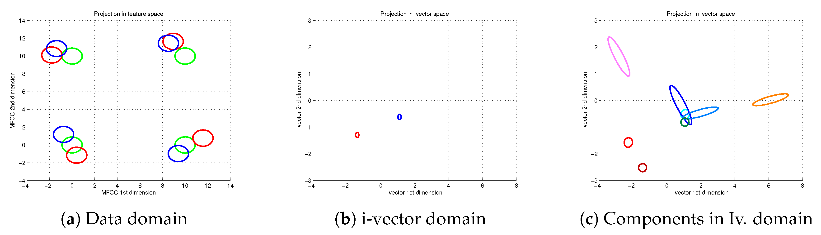
From the remaining data pool we choose two extra utterances, unseen during the model training, for evaluation purposes. Because these two utterances are independent, we assume them to represent two different speakers. In Figure 1 we represent them, red and blue respectively. The representation includes three parts: In the first part we show the original feature domain, that is, the utterance set of feature vectors. Each ellipse in the figure represents the distribution of each Gaussian in their GMMs. The image also includes in green the representation of the UBM model. The second part in Figure 1 represents the same red and blue utterances in the latent space by means of the posterior distribution of the latent variable $\mathbf{w}$. The third part of Figure 1 illustrates the location of the particular estimations per component $G_i\left(\mathbf{A}\right)$ for the two utterances in the latent space. Reddish estimations correspond to the red speaker while bluish ellipses represent the phonemes for the blue speaker.

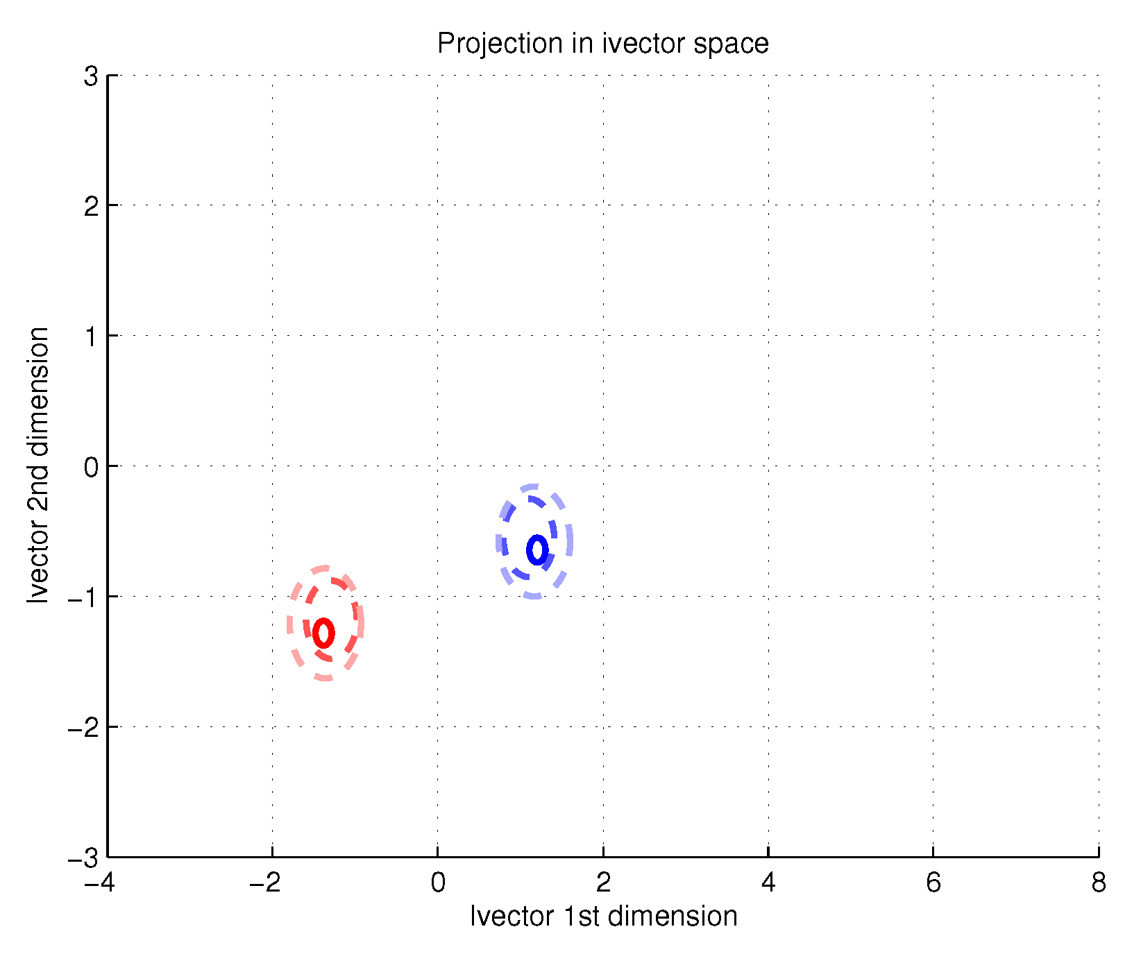
Following the described setup we can carry out an analysis of degradation in short utterances. First we illustrate the phoneme dependent estimation error due to limited data. For this reason we estimate the posterior distribution of the embeddings for multiple utterances only differing the number of samples. The distribution of phonemes $\mathit{\alpha }$ remains unaltered. Theoretically, the embeddings should not suffer any bias but its uncertainty should get larger as long as the utterances contain less data. In Figure 2 we compare the original utterances to those obtained with one fifth of the data and one tenth of the data.

Figure 2 illustrates the posterior distribution of the latent variable for the short utterances (dashed-line red and blue ellipses) as well as the original utterances (red and blue ellipses with continuous line respectively). The location of the ellipse represents the mean of the posterior distribution while its contour the uncertainty. As expected, the original reference utterance and their shorter versions present very reduced shifts among themselves, with almost concentric ellipses. While the blue speaker suffers almost no degradation, the red speaker biases are more noticeable. Besides, the illustration shows that the less data in the utterance, the bigger the uncertainty of the estimation.

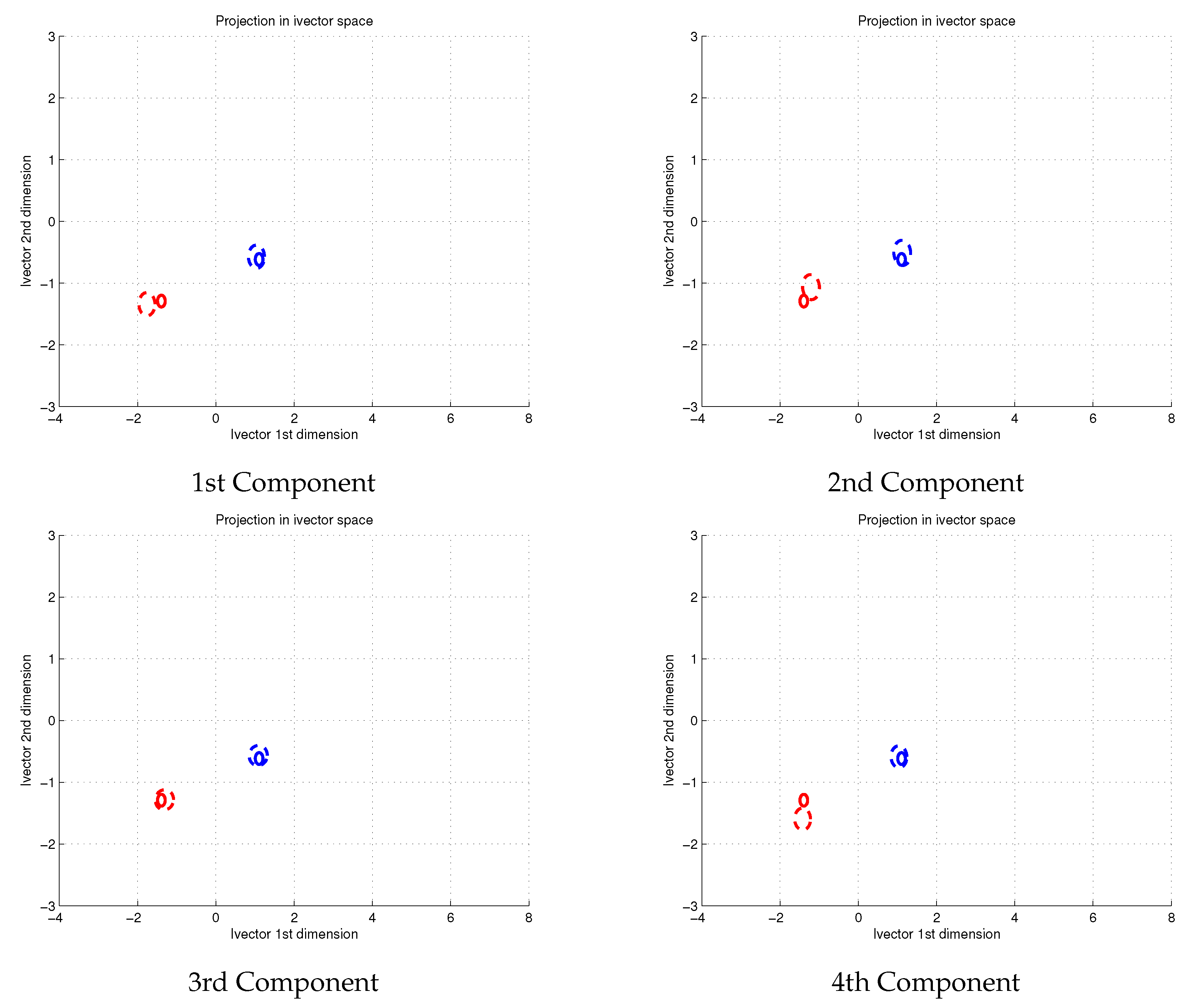
Now we study the impact of the distribution of acoustic units $\mathit{\alpha }$ on the embedding. In the reference utterances this distribution was uniform, this is, $25\%$ of the samples came from each component. We now modify this distribution for both utterances, red and blue. In Figure 3 we show the posterior distributions of the original utterances (red and blue ellipses with continuous line) as well as the altered short utterances (dashed-line red and blue ellipses). In the illustrated example half of the feature vectors are sampled from a single component of the GMM while the remaining data is evenly sampled along the other components. We have studied the effect with the four components in the GMM.

Illustrated results in Figure 3 reveal the relevance of the distribution of phonemes $\mathit{\alpha }$ for its proper modelling. The modification of the distribution of weights makes the red speaker to offer four different representations of the same embedding. Besides, these representations are not overlapped among themselves, beyond the uncertainty region from the original utterance. Therefore, these alternative embeddings are likely to fail. Nevertheless, not all speakers behave equally. Whilst red speaker is degraded, our blue speaker has suffered the same alterations without any visible shift on his/her embeddings.

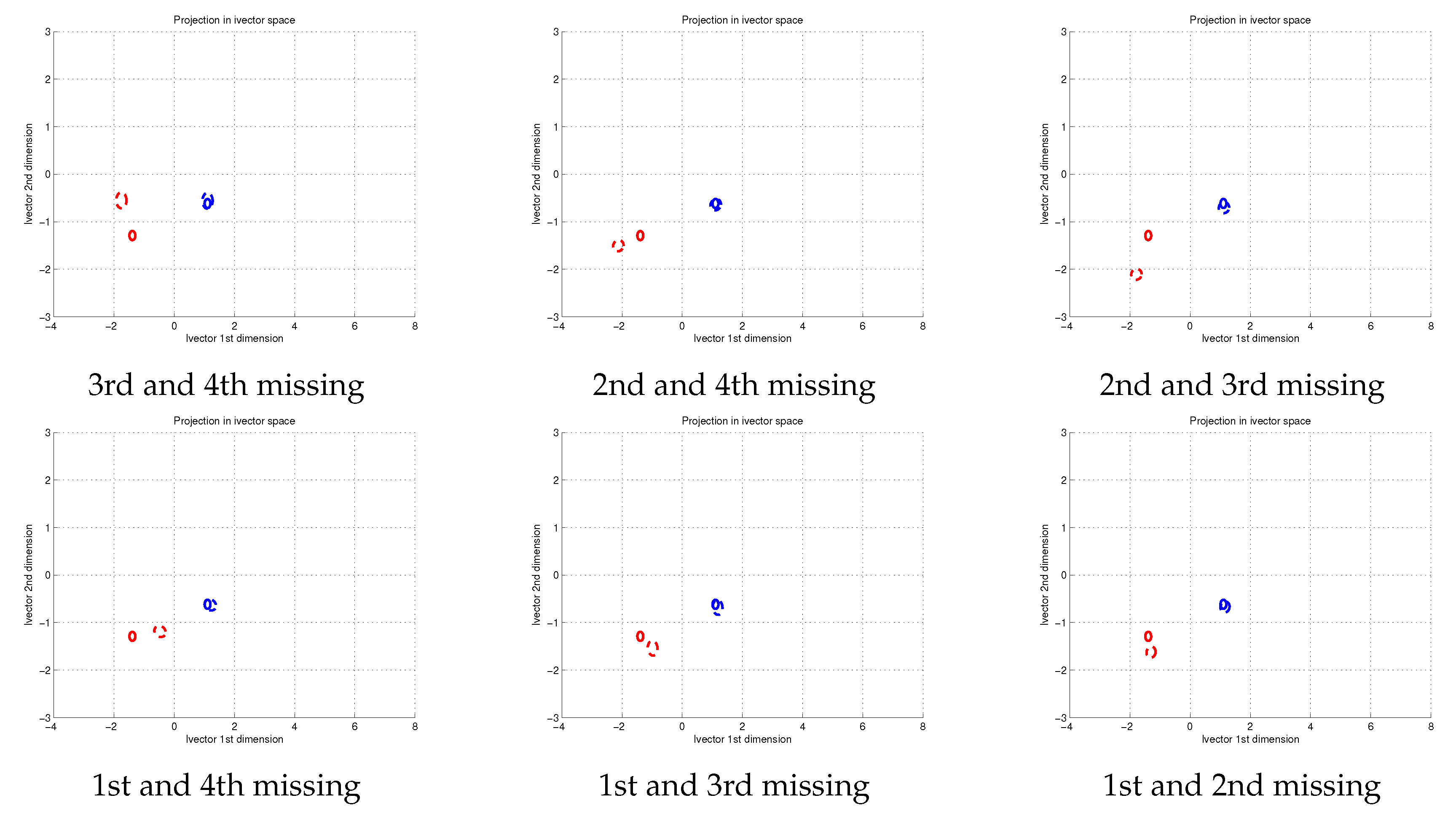
The scenario with a distorted phoneme distribution can be taken to the limit. In this situation some components do not contribute to the final embedding. This scenario is the most adverse, significantly modifying the distribution of patterns $\mathit{\alpha }$ and some estimations per phoneme $G_i\left(\mathbf{A}\right)$ being set to zero. In this experiment we have disturbed the distribution of acoustic units $\mathit{\alpha }$ forcing two of the components to zero. In Figure 4 we illustrate the six possible scenarios in terms of the non-contributing components. The results are shown for the two test speakers red and blue, with continuous line ellipses for the reference utterances and dashed-line ellipses for their altered versions.

According to the representations shown in Figure 4, embeddings from utterances with missing components experiment large biases with respect to the reference embeddings. These shifts are more significant than those previously seen with less extreme distortions in the phoneme distribution $\mathit{\alpha }$. Some of the hypothesized embeddings are far beyond the uncertainty from the original utterance. The biases suffered by the utterances are not the same for both speakers. Again the blue speaker suffers no relevant degradation. This behaviour fits in our hypothesis because the missing components scenario is the limit case of phoneme distribution degradation.

In all our experiments the red speaker has suffered from strong degradations while the blue speaker has remained almost unaltered. This different behaviour is a consequence of the locations of the phonetic estimations $G_i\left(\mathbf{A}\right)$ for each speaker. On the one hand, as shown in Figure 1, our blue speaker has its components very close to each other, providing robustness against distribution modifications. On the other hand our red speaker has its components much further from each other. Therefore, any alteration of the distribution implies a much more significant degradation in the location of the red speaker. In consequence, some speakers will be more robust to short utterances modifications than others.

5. Experiments & Results

Our hypothesis is that short utterances work well in evaluation if both enrollment and test contain similar phonetic content, being degraded otherwise. According to our previous analysis with artificial data, embeddings from short utterances can suffer from biases due to a mismatch in the distribution of acoustic units $\mathit{\alpha }$ and the effect of missing components $G_i\left(\mathbf{A}\right)$. Therefore, evaluation of trials should behave better if both enrollment and test embeddings were similarly altered.

5.1. Experimental Setup

Our experimental work is constructed around the SRE10 “coreext-coreext det5 female” experiment. This experiment, part of the Speaker Recognition Evaluation 2010 [15] proposed by the National Institute of Standards and Technology (NIST), requires the scoring of more than two hundred fifty thousand trials, recorded from telephone channel in the United States. Each trial consists of two utterances, enrollment and test, with about three hundred seconds of audio per role. Each utterance is known to contain a single speaker. Evaluation rules impose no restriction about the treatment of each trial, but it is obligatory to treat trials independently, not transferring any knowledge among them.

In this work we restrict our efforts to i-vectors. This choice was taken for illustrative purposes. Therefore, 20 MFCC feature vectors, with first and second order derivatives and Short Time Gaussianization [32] are applied. Utterances are then represented by a gender dependent 2048-Gaussian UBM trained with excerpts from SRE 04, 05, 06 and 08. Based on this UBM a gender dependent 400-dimension T matrix is trained, also using excerpts from SRE 04, 05, 06 and 08. The obtained embeddings, in this case i-vectors, are centered, whitened and length-normalized [33]. The back-end consists of a 400 dimension Simplified PLDA. No score calibration is applied, so results are measured in terms of Equal Error Rate (EER) and minDCF. This latter measure is based on the Detection Cost Function (DCF)

$$DCF=C_{\mathrm{Miss}}P\left(\mathrm{Miss}\right)P\left(\mathrm{Target}\right)+C_{\mathrm{F}.\mathrm{A}.}P\left(\mathrm{F}.\mathrm{A}.\right)(1-P\left(\mathrm{Target}\right))$$

(8)

This function weights the probability of missing a target ($P\left(\mathrm{Miss}\right)$) and the probability of producing a false alarm ($P\left(\mathrm{F}.\mathrm{A}.\right)$) to set them in the operating point, fixed by the cost of each kind of error ($C_{\mathrm{Miss}}$ and $C_{\mathrm{F}.\mathrm{A}.}$ respectively) and the prior probability of a target trial $P\left(\mathrm{Target}\right)$. For the evaluation, the defined operating point forces the values for the three parameters to be 10, 1 and 0.01 respectively.

In this work we need to measure the relative differences in the phoneme distribution between enrollment and test. Hence we must define a metric to measure how close these two utterances are from each other. In this work we have opted for the KL2 distance [34]. This metric, based on the Kullback Leibler (KL) divergence, determines how distribution q differs from distribution p. The KL divergence for discrete random variables is formulated as follows:

$$D_{\mathrm{KL}}(p,q)=\sum _{i}p\left(i\right)ln\frac{p\left(i\right)}{q\left(i\right)}$$

(9)

The KL divergence is not simmetric, thus we apply its symmetric version, the KL2 distance.

$$D_{\mathrm{KL}2}(p,q)=D_{\mathrm{KL}}(p,q)+D_{\mathrm{KL}}(q,p)=D_{\mathrm{KL}2}(q,p)$$

(10)

In i-vectors the phoneme distribution $\mathit{\alpha }$ matches the responsibility distribution. Consequently, our KL2 metric is evaluated between the responsibility distribution of enrollment and test. This distribution can be obtained from the zeroth order Baum-Welch statistic.

5.2. Baseline

Our first experiment sets a benchmark based on the SRE10 “coreext-coreext det5 female” experiment. This experiment only includes utterances with approximately 300 s of audio. Hence, in order to illustrate the degradation of short utterances we have considered two datasets obtained from the same utterances.

• Long. The original utterances provided by the organizers for the evaluation, with approximately 5 min of audio per utterance. These utterances play the role of long reference utterances.
• Short Random. An alternative version of the original SRE10 dataset with restricted information. Each utterance of the original dataset is chopped restricting its audio speech to be in the range 3–60 s. The chop marks, starting point and initial position were randomly chosen. Utterance chopping was done after Voice Activity Detection (VAD). These utterances can suffer from degradation due to errors in the phoneme estimations $G_i\left(\mathbf{A}\right)$ and mismatch in the phoneme distribution $\mathit{\alpha }$.

Thanks to these two datasets we have available a version of the utterances with full information and a version with partial knowledge. Now we must define the scenarios for the evaluation, assigning the roles of enrollment and test. We are interested in three particular scenarios:

• Long-Long. The official NIST SRE10 experiment. The Long dataset plays both roles, enrollment and test, in each trial. This experiment represents the case in which we have complete information for both speakers.
• Long-Short. In this scenario the Long dataset also plays the role of enrollment, while the shortened dataset is used for test. In this scenario we study the scenario where the reference speaker, the enrollment, is perfectly characterized while the candidate (the test) speaker is unreliably represented.
• Short-Short. The Short Random dataset plays both roles, enrollment and test. This scenario reveals the performance with very limited information.

The three scenarios are evaluated by means of the same trial list, which defines the comparisons to evaluate. The only difference among scenarios is the particular audio within the utterance to model the speakers. The results with these three configurations can be seen in

Table 1. Results, EER (%) and minDCF of SRE10 “coreext-coreext det5 female” experiment with the three scenarios of interest: Long-Long, Long-Short and Short-Short.

Scenario	EER(%)	MinDCF
Long-Long	3.25	0.16
Long-Short Random	5.67	0.27
Short-Short Random	8.57	0.40

.

These results confirm that short utterances degrade performance. Besides, as long as more and more data are represented by means of short utterances, we suffer more degradation. This degradation affects both evaluation metrics EER and minDCF.

5.3. Reduction of the Mismatch in $\alpha$: Phonetic Balance

In our previous analysis we hypothesized two main sources of degradation in short utterances: The one due the uncertainty in the phoneme estimations $G_i\left(\mathbf{A}\right)$ and another term caused by mismatches in the phoneme distribution $\mathit{\alpha }$. In order to test our hypothesis we are going to minimize the errors due to phoneme distribution $\mathit{\alpha }$. To do so we have prepared an extra dataset, named as Short Balanced. This dataset is also obtained from the original data released by the organization. From each original utterance we obtain phoneme labels, one per input feature vector. These phoneme labels in this experiment were obtained by automatic means, that is, a DNN phoneme classifier [35] consisting of a Wide Residual Network [36] with four blocks. Only 39 phoneme labels were considered, that is, each phoneme label includes all its associated coarticulation. Experiments carried out in TIMIT [37] show error rates around 15% in the classification task.

The phoneme labels in an utterance determine its phoneme distribution. This distribution, obtained from the long utterance, must be maintained in the new short utterance despite its lower length. Therefore, given the length of the new short utterance we can determine the newer number of samples per phoneme. Then we randomly choose this number among the all the samples with a certain phoneme, repeating the process for all phonemes. Frames must be considered speech by our VAD to be candidate for the new utterances. For comparison reasons each Short Balanced utterance contains as many samples as in the Short Random counterpart.

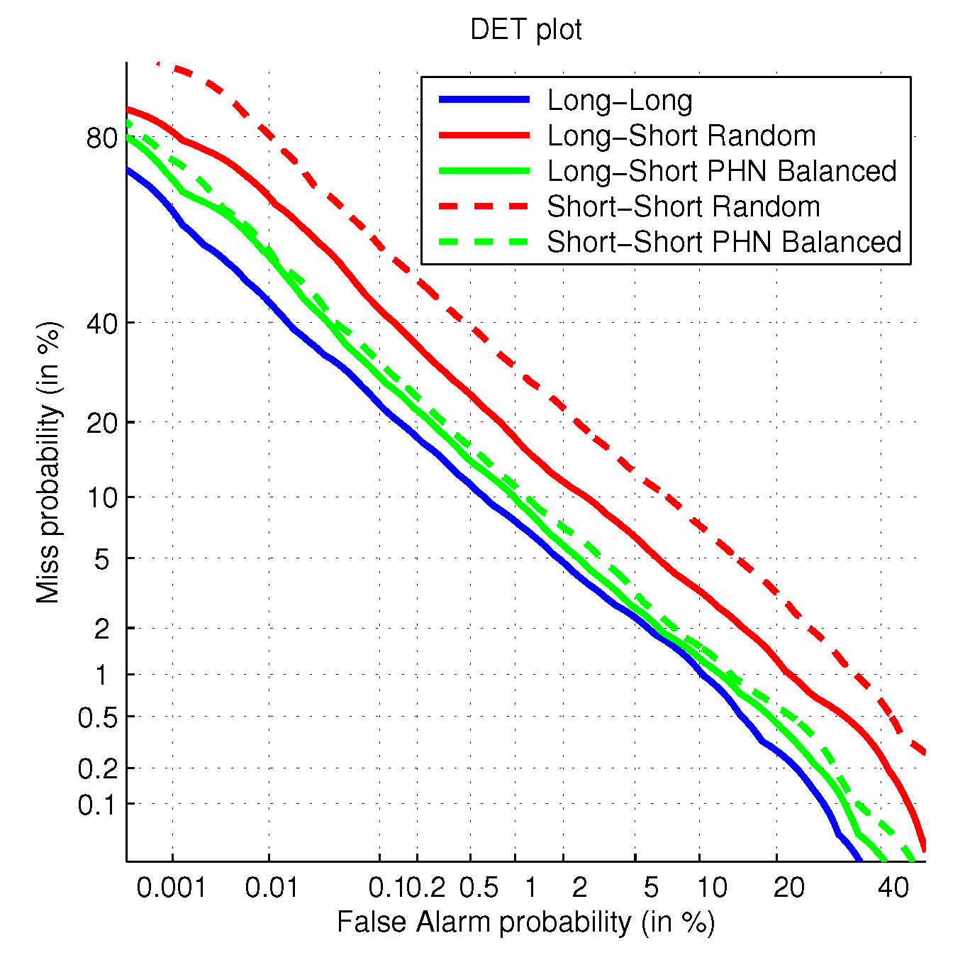
The comparison between both types of short utterances is shown in

Table 2. Comparison of results, EER(%) and minDCF, between Short-Random and Short Balanced dataset in SRE10 “coreext-coreext det5 female” for scenarios Long-Short and Short-Short.

Scenario	EER(%)	MinDCF
Long-Short Random	5.67	0.27
Long-Short PHN Balanced	3.62	0.19
Short-Short Random	8.57	0.40
Short-Short PHN Balanced	4.11	0.20

. The comparison includes the results in the Long-Short and Short-Short scenarios. This information is complemented with the Detection Error Tradeoff (DET) curves in Figure 5, where we also include the Long-Long scenario for comparison reasons.

According to the shown results, the new Short Balanced dataset is able to behave much better than the Short Random dataset, despite containing both datasets the same amount of speech. This is because the phonetic balance with respect to the original utterance also reduces the distance between enrollment and test phoneme distributions $\mathit{\alpha }$. Therefore, we get rid of this source of error, only remaining those errors due to the phoneme estimations $G_i\left(\mathbf{A}\right)$. We have also realized that the degradation due to the phonetic distribution mismatch is much more relevant than those related with the uncertainty of the estimations $G_i\left(\mathbf{A}\right)$.

In order to obtain a better understanding we analyze the already obtained results in terms of the type of trial: target and non-target. This study compares the KL2 distance between enrollment and test with respect to the probability of error in each population. In this work the KL2 distance measures how the responsibility distributions for enrollment and test utterances match each other. The obtained results are shown in

Table 3. Kullback Leibler (KL) distance and Error (%) for both target and non-target trials in experiments Long-Long, Short Short Random and Short-Short Balanced. Error estimated at National Institute of Standards and Technology (NIST) operating point.

Experiment	KL2 Distance (nats)		Population Error (%)
	Target	Non-Target	Target	Non-Target
Long-Long	1.06	1.74	28.43	0.06
Short-Short Random	3.62	4.61	80.40	0.01
Short-Short Balanced	2.55	3.47	40.79	0.03

. This analysis is performed for the experiments Long-Long, Short-Short Random and Short-Short Balanced. Besides, we study the impact of the KL2 to the classification error in target and non-target trials, that is, the Miss and False Alarm error terms. The decision threshold is set up according to the operating point defined by the evaluation.

Results in Table 3 illustrate many details. First, the KL2 distance increases for both target and non-target trials as long as we move from the Long-Long experiment to the Short-Short Balanced and finally the Short-Short Random experiment. Besides, this KL2 distance is always higher in the non-target trials population than in target trials. Moreover, regardless of the utterance length or content, evaluation errors are mainly caused by the misclassification of target trials. We also see some correlation between the relative KL2 distances and the errors. In target trials the lower the distance, the lower the error in the target population. These results also illustrate that our Short Balanced dataset obtains its improvement mainly from the target trials, halving their error. With respect to the non-target trials, we see a negative correlation, with an error term deceasing as long as the KL2 metric increases.

Finally, combining the information of Table 2 and Table 3 we realize that the relationship between the relative KL2 distance and the error metrics EER and minDCF is not linear. We carried out a linear regression of the evaluation results (EER and minDCF) in terms of the KL2 distance. This regression was estimated in terms of the obtained results for the Long-Long and Short-Short Random experiments. When we infer the results for the Short-Short Balanced experiment according to its KL2 distance, those are significantly worse than the really obtained ones. According to this regression this experiment should have obtained 6.33% EER and 0.30 minDCF, far higher than the obtained values. Therefore, the distance/EER and distance/minDCF relationships should be steeper with higher KL2 values and more even with the lower distances.

5.4. Enrollment-Test Distance versus Log-Likelihood Ratio (LLR)

Our previous experiments reveal the relationship between the relative distance in terms of phonetic content between enrollment and test utterances and the performance of these trials. Thus, we explore the impact of this distance in the performance.

For this analysis we opt for the Short-Short scenario. The test role in each evaluation is always played by an utterance from the Short Random dataset. Regarding the enrollment role, we have created the following pool of data, with multiple candidate utterances for each trial:

• The Short Random dataset experiment previously analyzed.
• Three alternative Short Random datasets. We chop the released original utterances in segments of the range 3–60 s of speech but now the chops are not totally random. They are restricted to differ from the test utterance in the trial a controlled KL2 value. These goal values for the distances are approximately 2, 3 and 4 nats.
• Short Equalized dataset. We equalize the original enrollment utterance to obtain a null relative distance between enrollment and test. By doing so we choose from the enrollment only those contents present in the test utterance and in the same proportion. The amount of audio is the same in both enrollment and test utterances.

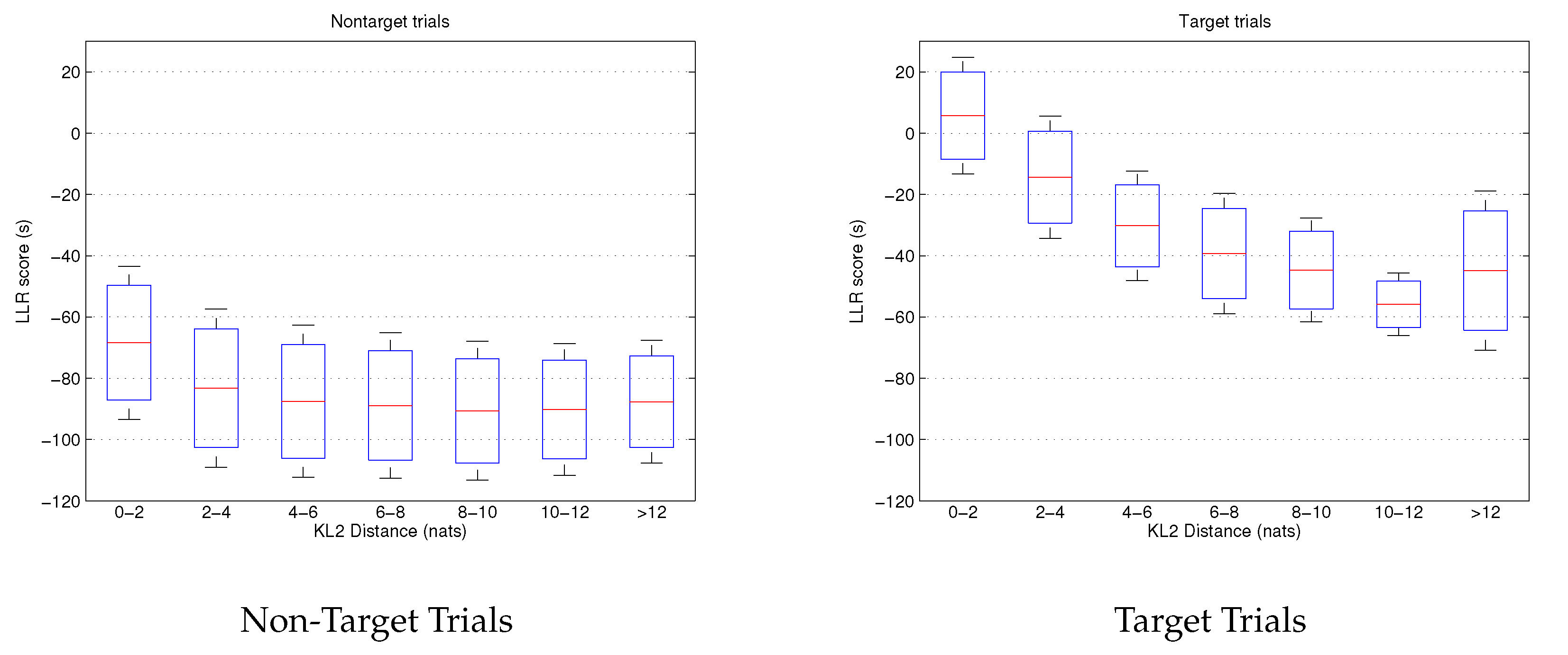
This large data pool allows the analysis of the relationship between enrollment-test relative distance and score. The results are visible in Figure 6. We present a boxplot of the log-likelihood ratio score in terms of the distance in bins of 2 nats. Three values per bin are shown: the mean of the scores, the mean plus the standard deviation of scores and the mean minus the standard deviation of scores. He have differentiated between non-target trials and target trials for a better understanding.

Figure 6 confirms our previous conclusions. First, the score of target trials is strongly influenced by the relative phoneme distance between enrollment and test. The lower the distance, the higher is the score for the target trials. By contrast, non-target trials are almost insensitive to this distance. Their score remain steady for almost all the analysis. In conclusion, degradation is mainly caused by target trials, which strongly depend on the KL2 metric. However, Figure 6 indicates something more. Non-target trials keep stable for almost all the distance range except for low values (0–2 nats), where the score increases. The very high phonetic similarity between enrollment and test utterances increases their log-likelihood ratio despite these trials do not contain the same speaker.

5.5. Enrollment-Test Distance versus Performance (Eer and Mindcf)

Previously we have studied the effect of relative phoneme distances on the score, individually analyzing each trial. Now we study the whole set of trials at once, providing the evaluation metrics, the Equal Error Rate (EER) and the minimum Decision Cost Function (minDCF).

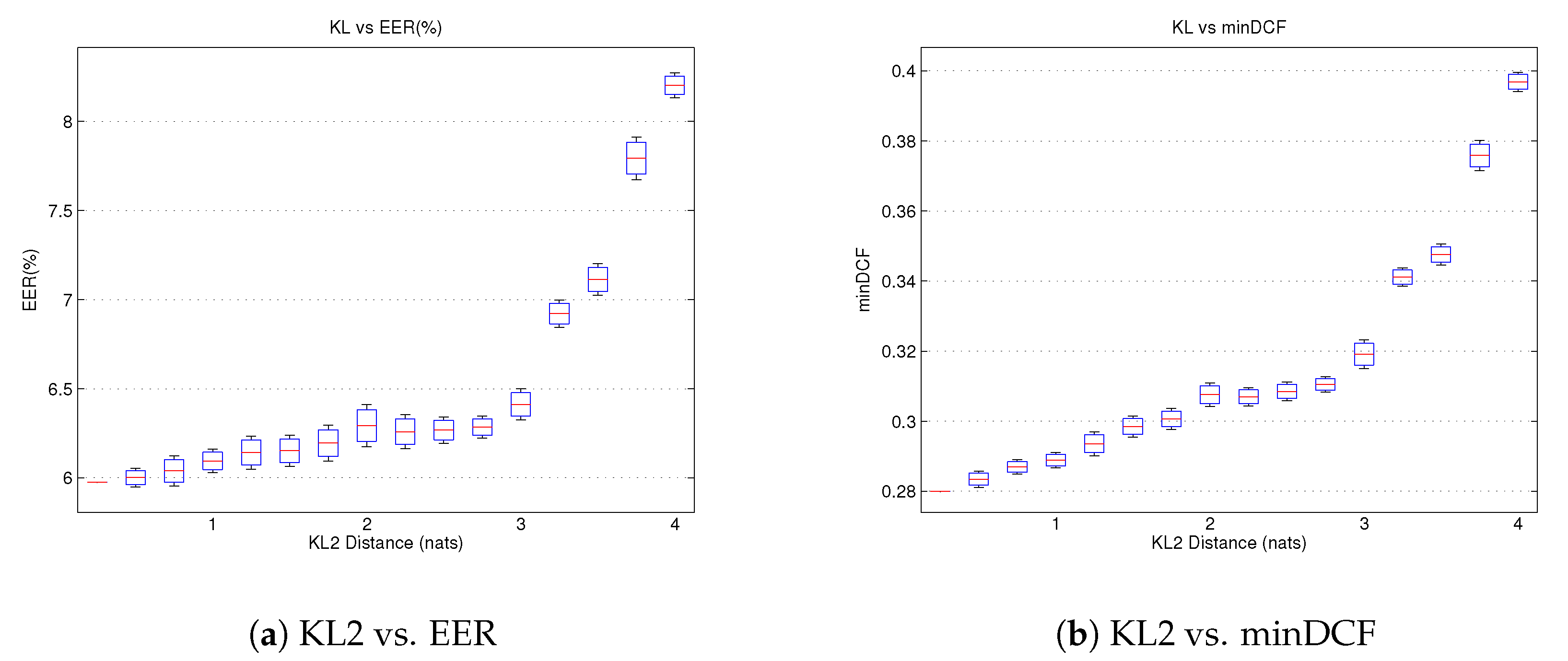
In Figure 7 we analyze the impact of the relative phonetic distance for the two evaluation metrics. For this purpose, we have conducted the SRE10 “coreext-coreext det5 female” experiment, selecting the scores for each trial from the previously described pool of scores. The results show the performance in terms of the average KL2 distance between enrollment and test trials. More than 10,000 different score sets were studied.

Figure 7 also confirms our previous conclusions. Previously we inferred a non-linear behaviour of the EER and minDCF with respect to the relative phoneme distance. We realized that low values of phoneme distance should generate low degradations, getting more relevant as long as the KL2 distance increases. Figure 7 shows an elbow shaped relationship with two different behaviours. Below a certain value, in this case approximately 3 nats, both evaluation metrics experiment low degradations (0.5% EER and 0.03 minDCF). However, once the relative phoneme distance exceeds this value, degradation increases rapidly. This elbow shape has great implications. By working within the lowest range of relative phoneme distance (in our case below 3 nats) we can assume a certain reliability in our results.

5.6. Long-Short versus Equalized Short-Short

Our experiments in the Short-Short scenario have revealed that utterances are better classified as long as the relative phonetic distance between enrollment and test decreases. Nevertheless, further information is available in other scenarios, as in the Long-Short scenario. While the short utterance has limited information in it, maybe missing some phonemes, the long utterance has complete information about all phonemes. Hence we must check whether this extra information is worthy or not.

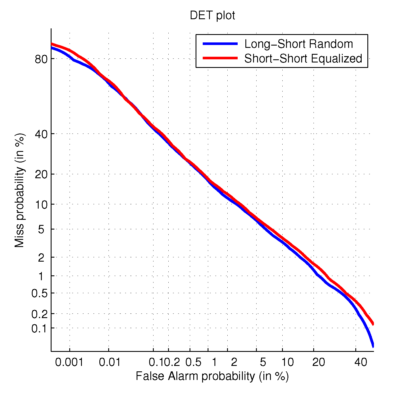
For this reason we compare the originally defined Long-Short experiment with the Short-Short experiment with lowest relative phoneme distance. This Short-Short experiment implies the equalization of the enrollment utterance to match the phonetic content in the test utterance, getting rid of any extra information. In this comparison both experiments share the same test utterances. The results for this experiment are shown in

Table 4. Comparion of results, EER(%) and minDCF, for scenarios Long-Short Random and Short-Short with equalized results. SRE10 “coreext-coreext det5 female experiment”.

Utterance	EER(%)	MinDCF
Long-Short	5.67	0.27
Short-Short Equalized	5.98	0.27

and DET curves are shown in Figure 8.

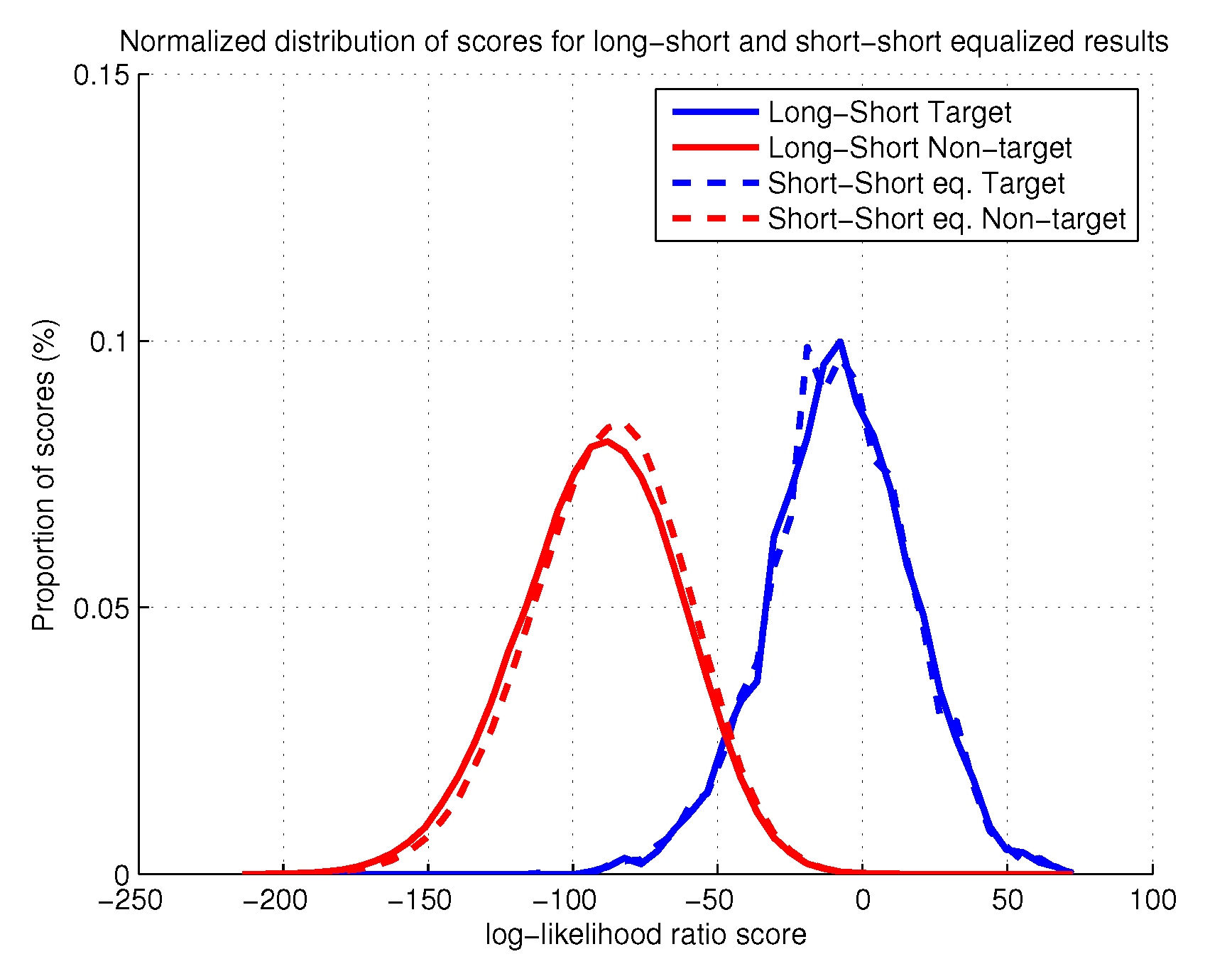
The results in both Table 4 and Figure 8 show that the extra information has a very small effect in the evaluation task. Nevertheless, despite both experiments have obtained very similar results, the Long-Short original experiment is slightly better. This issue can be partially justified by the range of the relative phoneme distances of the short-short experiment. The equalization imposes the relative distance to be equal to zero. In this range of values the non-target trials experiment an increase of the score, possibly causing the degradation. In order to confirm this explanation we analyze the score distribution for population of target and non-target trials in both experiments. These distributions are represented in Figure 9:

Figure 9 confirms our hypothesis of harmful non-target trials. The scores for the target trials overlap in both scenarios, Long-Short and Short-Short Equalized. By contrast, the score distribution for the non-target trials in the Short-Short equalized experiment is slightly positively biased with respect to the Long-Short counterpart. This extra deviation is responsible for the experimented small degradation of performance.

6. Conclusions

In this work we have successfully analyzed the problem of short utterances as a problem of unbalanced, even missing, patterns.

We have shown that embeddings can be partially understood as weighted sum of phoneme contributions, each of them illustrating the particularities of the speaker for the acoustic unit. When the weight distributions differ from the expected one as in short utterances, embeddings experiment shifts with respect to their original location. When these shifts are large enough they are not considered intra-speaker variability anymore and attributed to speaker mismatches. Therefore, these shifts are responsible for the loss of performance.

Our contribution has been focused on the phonetic similarity between enrollment and test utterances. We have proposed the KL2 distance as metric for the relative phonetic distance between enrollment and test. We have also illustrated the dependencies of the score and the evaluation performance (EER, minDCF) of systems in terms of the proposed distance. Moreover, we have realized that this influence is specially noticeable in the target trials, while non-target trials are almost unaffected. Our results also indicate the existence of a range of reliable distance where degradation is bounded. Working beyond this limit makes performance degrade very fast. Furthermore, our experiments indicate that once perfect match of the distributions is achieved, further information in extra components does not provide a significant improvement in performance.

Unfortunately, the phoneme distribution must be complemented with accurate information for all possible phonemes to be improved. Our experiments with very low relative phoneme distances, even zero, behave worse than experiments with complete information but larger enrollment-test distances. This is a consequence of the unseen phonemes, which help with the distance but not with the discrimination of speakers. Further research should be done about this missing information. Moreover, this analysis has been carried out with i-vectors. Therefore it is required experimental confirmation with other embedding representations in the state-of-the-art.