Towards Online Personalized-Monitoring of Human Thermal Sensation Using Machine Learning Approach

Abstract

Thermal comfort and sensation are important aspects of building design and indoor climate control, as modern man spends most of the day indoors. Conventional indoor climate design and control approaches are based on static thermal comfort/sensation models that view the building occupants as passive recipients of their thermal environment. To overcome the disadvantages of static models, adaptive thermal comfort models aim to provide opportunity for personalized climate control and thermal comfort enhancement. Recent advances in wearable technologies contributed to new possibilities in controlling and monitoring health conditions and human wellbeing in daily life. The generated streaming data generated from wearable sensors are providing a unique opportunity to develop a real-time monitor of an individual’s thermal state. The main goal of this work is to introduce a personalized adaptive model to predict individual’s thermal sensation based on non-intrusive and easily measured variables, which could be obtained from already available wearable sensors. In this paper, a personalized classification model for individual thermal sensation with a reduced-dimension input-space, including 12 features extracted from easily measured variables, which are obtained from wearable sensors, was developed using least-squares support vector machine algorithm. The developed classification model predicted the individual’s thermal sensation with an overall average accuracy of 86%. Additionally, we introduced the main framework of streaming algorithm for personalized classification model to predict an individual’s thermal sensation based on streaming data obtained from wearable sensors.

1. Introduction

Thermal comfort (TC) is an ergonomic aspect determining satisfaction with the surrounding environment and is defined as ‘that condition of mind which expresses satisfaction with the thermal environment and is assessed by subjective evaluation’ [1]. The effect of thermal environments on occupants might also be assessed in terms of thermal sensation (TS), which can be defined as ‘a conscious feeling commonly graded into the categories cold, cool, slightly cool, neutral, slightly warm, warm, and hot’ [1]. Thermal sensation and thermal comfort are both subjective judgements, however, thermal sensation is related to the perception of one’s thermal state, and thermal comfort is related to the evaluation of this perception [2]. In other words, TS expresses the perception of the occupants, while TC assesses this perception, taking into account physiological and psychological factors [3]. The assessment of thermal sensation has been regarded as more reliable and as such is often used to estimate thermal comfort [4].

Thermal sensation is the result of the body “psycho-physical reaction” to certain thermal stimuli related to indoor conditions [5]. Human thermal sensation mainly depends on the human body temperature (core body temperature), which is a function of sets of comfort factors [5,6]. These comfort factors include indoor environmental factors, such as mean air temperature around the body, relative air velocity around the body, humidity, and mean radiant temperature of the environment to the body [6]. Additionally, some personal (individual-related) factors, namely metabolic rate or internal heat production in the body, which vary with the activity level and clothing thermo-physical properties (such as clothing insulation and vapor clothing resistance), are included. It should be mentioned that the individual thermal perception is deepening, as well, on psychological factors, expectations and short/long-term experience, which directly affect individuals’ perceptions, time of exposure, perceived control, and environmental stimulation [7]. The most considered way to have an accurate assessment of TS is to ask the individuals directly about their thermal sensation perception [5,6]. The thermal-sensation-vote (TSV) is one of the most used concepts to address the opinion of individuals concerning TS. That is, individuals express their vote to rate their TS when they are exposed to given thermal conditions, by using a scale from cold to hot, with a predefined number of points.

Thermal sensation mathematical models are developed in order to overcome the difficulties of direct enquiry of subjects. The development of such models is mostly dependent on statistical approaches by correlating experimental conditions (i.e., environmental and personal variables) data to thermal sensation votes obtained from human subjects [4,6]. The recent intensive review work of Enescu (2019), explored the most important contributions to model and predict thermal sensation (TS) under both steady-state and transient conditions. It is shown that the most used models to assess TS of the human body with respect to the environment have been developed starting from Fanger’s predicted-mean-vote (PMV) empirical model [3] for steady-state conditions and from the Gagge model [8] for transient conditions. Since then, numurus models are developed to assess and predict TS (e.g., [9,10,11,12,13,14,15,16]). Most of the aforementioned models (e.g., PMV) are static in the sense that they predict the average vote of a large group of people based on the seven-point thermal sensation scale, instead of individual thermal comfort, they only describe the overall thermal sensation of multiple occupants in a shared thermal environment. To overcome the disadvantages of static models, adaptive thermal comfort models aim to provide insights in increasing opportunities for personal and responsive control, thermal comfort enhancement, energy consumption reduction and climatically responsive and environmentally responsible building design [17,18]. The idea behind adaptive models is that occupants and individuals are no longer regarded as passive recipients of the thermal environment but rather, play an active role in creating their own thermal preferences [18]. Many adaptive thermal comfort models are developed based on regression analysis (e.g., [18,19,20]).

Besides regression analysis, thermal sensation prediction can also be seen as a classification problem where various classification algorithms can be implemented [17]. In their work [21], Lee et al., proposed a method for learning personalized thermal preference profiles by formulating a combined classification and inference problem with 5-cluster models. Moreover, the thermal preference of a new user is inferred by a mixture of sub-models for each cluster, where clusters are used to group occupants with similar thermal preferences.

Recently, a number of research works (e.g., [22,23,24,25,26] have demonstrated the possibility of using machine learning techniques, such as support vector machine (SVM), to assess and predict human thermal sensation. It can be concluded, based on the published work (see the recent literature review [17] by Lu et al.), that classification-based models have performed as well as regression models.

Different related works investigated the problem of thermal sensation and comfort prediction via machine learning algorithms. Ghahramani et al. [27] applied the hidden Markov model (HMM) technique to the thermal comfort prediction problem with three levels of thermal comfort. There is a main issue in the used dataset in this study is the class imbalance, which is not tackled by the proposed methodology. In their study, Ghahramani et al. did not discuss the problem of streaming analytics and model personalisation.

In order to develop personalized models, Jiang et al. [28] applied support vector machines classifiers to the personal data of each subject to predict the thermal sensation level for the same subject. The obtained results are promising, however, their approach requires a sufficient number of data-points to obtain an acceptable performance, which is not applicable to our dataset (9 data-points per subject).

The very recent study of Lu et al. [17] proposed a personalized model, however, the study strictly investigated two subjects and developed a dedicated model for each subject.

In comparison with many relevant studies, our study is tackling several challenges at the same time. These issues are feature reduction, streaming, and online modeling compatibility and model personalization. The latter issue is tackled in a novel way by considering both personal and nonpersonal data relying on the similarity either inter or intra subjects. In general, it can be stated that it is a real modeling challenge to correlate the physiological variables with information concerning global and local sensation [5].

Recent advances in mobile technologies in healthcare, in particular, wearable technologies (m-health) and smart clothing, have positively contributed to new possibilities in controlling and monitoring health conditions and human wellbeing in daily life applications. The wearable sensing technologies and their generated streaming data are providing a unique opportunity to understand the user’s behaviour and to predict future needs [29]. The generated streaming data is unique due to the personal nature of the wearable devices. However, the generated streaming data forms a challenge related to the need for personalized adaptive models that can handle newly arrived personal data.

The main goal of this work is to introduce a personalized adaptive modeling algorithm to predict an individual’s thermal sensation based on non-intrusive and easily measured variables, which could be obtained from already available wearable sensors.

2. Methods

2.1. Data Processing and Classification

Thermal sensation prediction based on wearable sensors can be considered as a classification machine learning problem, the input of which is the set of extracted features from the measured variables and the output is the subjects’ feedback with the standard thermal sensation labels. Several machine learning techniques can be used for such a problem. Support vector machines (SVMs) is one of the efficient classification techniques used in different relevant studies [21,22,23,25,26]. In this study, the least squares support vector machine (LS-SVM) is proposed to be used for general models as it is as powerful as standard SVMs, but, it has less computational cost [30]. Most, if not all, relevant studies of thermal sensation prediction rely on global general models. Global models are models that are trained using the whole available training dataset with a uniform weight (i.e., all training points are equally contributing to the training process). However, global models are not that efficient for online classification and streaming analytics applications in which a stream of new data is collected from subjects via wearable technology, especially when aiming at personalized models. Hence, for this purpose, we suggest a localized version of LS-SVM, namely K-Nearest Neighbours (KNN)-LS-SVM [31] to be compatible with the wearable sensors for online and streaming analytics.

The classification problem of thermal sensation is a multiclass classification problem, the input variables of this problem from which features are extracted are: aural temperature $T_{er}$, average skin temperature ${\overline{T}}_{sk}=\frac{1}{3}\left[T_{scap}+T_{ch}+T_{arm}\right]$, ambient temperature $T_a$, chest skin temperature $T_{ch}$, heart rate $H_r$, average heat flux from the skin ${\overline{q}}_{sk}$, temperature gradient between core and skin $\Delta T_{sk}=T_{er}-{\overline{T}}_{sk}$, age, gender, body mass index $BMI$, metabolic rate $M_r$. As some variables are time measurements of the different parameters, the process of feature extraction is applied to a specified time window from the recordings, namely the last five minutes preceding the sensation labeling by the test subjects. The extracted features from time-variant variables are: minimum ($min$), maximum ($max$), variance ($var$), energy, time-derivate ($\frac{\mathit{d}}{\mathit{d}\mathit{t}}$), root mean square ($rms$). Target labels are the seven classes of the standard thermal comfort sensation scores: Cold (-3), Cool (-2), Slightly Cool (-1), Neutral (0), Slightly Warm (1), Warm (2), and Hot (3).

2.1.1. Support Vector Machines (SVMs)

SVMs are originally presented as binary classifiers, that assign each data instance $X\in$ ${ℝ}^d$ to one of two classes described by a class label $y\in \left\{-1,1\right\}$ based on the decision boundary that maximizes the margin $2/{\parallel w\parallel }_2$ between the two classes. Generally, a feature map $\varphi :{ℝ}^d\underset{}{\Rightarrow }{ℝ}^p$ is used to transform the geometric boundary between the two classes to a linear boundary $L:{\mathbf{w}}^T\phi \left(x\right)+b=0$ in feature space, for some weight vector $\mathbf{w}\in {ℝ}^{p\times 1}andb\in ℝ$. The class of each instance can then be found by $y=sign\left({\mathbf{w}}^T\phi \left(x\right)+b\right)$, where $sign$ refers to the sign function [30].

The estimation of the boundary $L$ is performed based on a set of training examples $x_i\left(1\le i\le N\right)$ with corresponding class labels $y_i\in \left\{-1,1\right\}$. An optimal boundary is found by maximizing the margin that is defined as the smallest distances between $L$ and any of the training instances. In particular, one is interested in constants $\mathbf{w}$ and $b$ that minimize a loss-function:

$$\underset{\mathrm{w},\mathrm{b};\mathsf{\xi }}{\min } \frac{1}{2}{\mathbf{w}}^T\mathbf{w}+C{\displaystyle \sum }_{\mathrm{i}=1}^N{\xi }_i$$

(1)

and are subject to:

$$y_i\left({\mathbf{w}}^T\phi \left(xi\right) + b\right)\ge 1 - {\xi }_i and {\xi }_i \ge 0, i = 1, 2, \mathrm{...}, N.$$

(2)

The constant $C$ denotes the penalty term that is used to penalize misclassification through the slack variables ${\xi }_i$ in the optimization process.

The so-called kernel-trick avoids the explicit introduction of a feature map $\varphi$ and implicitly allows for the use of feature spaces of infinite dimensionality. A commonly used kernel is given by the Gaussian kernel:

$$k\left(x_i ,x_j \right)=exp \left(\frac{{\left|\left|x_i-x_j \right|\right|}^2}{2{\sigma }^2}\right)$$

(3)

where $\sigma$ denotes the kernel bandwidth. Both $\sigma$ and $\mathrm{C}$ can be optimized as hyper-parameters in a cross-validation experiment.

2.1.2. Least Squares Support Vector Machine (LS-SVM)

LS-SVMs are obtained by using a least-squares error loss function [30]:

$$\underset{\mathrm{w},\mathrm{b};e}{\min } \frac{1}{2}{\mathbf{w}}^T\mathbf{w}+\gamma {\displaystyle \sum }_{\mathrm{i}=1}^N{e}_i^2$$

(4)

such that

$$y_i\left({\mathbf{w}}^T\phi \left(x_i\right) + b\right)\ge 1 - e_i and e_i \ge 0, i = 1, 2, \mathrm{...}, N.$$

(5)

This optimization procedure introduces errors $e_i$ such that 1−$e_i$ is proportional to the signed distance of $x_i$ from the decision boundary and$\mathsf{\gamma }$ represents the regularization constant. In fact, the non-negative slack variable constraint is removed and the solution of the optimization problem can be obtained by a set of linear equations, reducing computational effort [30].

2.1.3. KNN-LS-SVM

While global SVMs consider the same weight for all training instances in the optimization process, local learning approaches allow for training samples near a test point to be more influential than others. Localized approaches of SVMs [31] are based on weighting functions $\lambda \left(x_s, x_i\right)$ that express the similarity between the features vectors of the $i$^th data point $x_i$ and the test instance $x_s$. For an LS-SVM, this leads to the following cost function:

$$\underset{\mathrm{w},\mathrm{b};e}{\min } \frac{1}{2}{\mathbf{w}}^T\mathbf{w}+\gamma {\displaystyle \sum }_{\mathrm{i}=1}^N\lambda \left(x_s, x_i\right)e_i^2$$

(6)

such that

$$y_i\left({\mathbf{w}}^T\phi \left(x_i\right) + b\right)\ge 1 - e_i and e_i \ge 0, i = 1, 2, \mathrm{...}, N.$$

(7)

For KNN-LS-SVM a binary valued similarity criterion:

$$\lambda \left(x_s, x_i\right)=\{\begin{array}{c}1 \mathrm{if} {\left|\left|\mathsf{\phi }\left(x_s\right)-\mathsf{\phi }\left(x_i\right) \right|\right|}^2 \le r_s\\ 0 \mathrm{otherwise} \end{array}$$

(8)

where $r_s$ is the $K^{\mathrm{th}}$ smallest distance among {||$\mathsf{\phi }\left(x_s\right)-\mathsf{\phi }\left(x_i\right)$||; 1 ≤ j ≤ N}. This formulation leads to the hybrid KNN-LS-SVM method [31]. In practice, implementing the hybrid classifier of KNN-LS-SVM, as shown in Figure 1, starts with receiving an unlabelled new test point $x_s$ and finding the nearest $K$ points from the training set in the feature space. Based on the nearest $K$ points, an LS-SVM model is trained only with the new subset, hence, for each test point a dedicated model is trained. The advantage of this localized approach is that it can enhance the classification performance in case of class imbalance, in addition to the computational and temporal efficiency especially for online modelling and streaming analytics. For more detail concerning localized learning, reference [31] includes a detailed explanation of the algorithms.

2.2. Experiments and Experimental Setup

2.2.1. Test Subjects

In total 25 healthy participants (6 females and 19 males), between the age of 25 and 35 (average age 26 ± 4.2) years, with average weight and height of 70.90 (± 12.70) kg and 1.74 (± 0.10) m, respectively, volunteered to perform the aforementioned experimental protocol. Detailed physical information about the test subjects is shown in

Table 1. General physical information of the participants (test subjects).

Subject	Gender	Height (cm)	Weight (kg)	Age (year)
P1	M	1.69	59	23
P2	M	1.77	75	20
P3	M	1.82	73	29
P4	F	1.61	53	31
P5	M	1.86	88	21
P6	F	1.57	50	22
P7	M	1.73	86	33
P8	M	1.81	67	21
P9	M	1.86	92	36
P10	M	1.65	62	31
P11	F	1.7	61	23
P12	M	1.86	80	23
P13	M	1.82	86	27
P14	F	1.6	51	22
P15	M	1.7	58	29
P16	M	1.75	74	26
P17	F	1.68	76	26
P18	M	1.8	74	29
P19	M	1.78	79	29
P20	M	1.83	81	22
P21	M	1.78	78	28
P22	M	1.81	69	22
P23	F	1.57	49	26
P24	M	1.75	68	24
P25	M	1.78	83	28

.

2.2.2. Climate Chambers

During the course of this study, three (Rooms A, B and C) climate-controlled chambers designed and built to investigate the dynamic mental and physiological responses of humans to specific indoor climate conditions were used. Figure 2 shows a photographic picture of the three climate rooms, namely, A, B and C. The Body and Mind Rooms are experimental facilities at the M3-BIORES laboratory (Division of Animal and Human Health Engineering, KU Leuven). The three rooms are dimensionally identical; however, each room is designed to provide different ranges of climate conditions as shown in

Table 2. Different temperature and relative humidity ranges that can be provided by the different Body and Mind (A, B and C).

Room	Air Temperature Range (°C)	Relative Humidity Range (%)
A	+23–+37	50–80
B	+10–+25	50–80
C	−5–+10	40–60

.

The three rooms are equipped with axial fans to simulate wind velocities between 2.5 and 50 km h⁻¹.

2.2.3. Measurements and Gold Standards

During the course of the experiments, participants’ heart rate $H_R$, metabolic rate $M_r$, average skin temperature $T_{sk}$, heat flux $q_{sk}$ between the skin and the ambient air, core body temperature $T_c$ represented by the aural temperature$T_{er}$were measured continuously. The heart rate of each participants was monitored with a sampling rate of 128 Hz using the Polar H7 ECG strap that is placed under the chest. The metabolic rate as metabolic equivalent tasks (METs) of each participant was calculated based on indirect calorimetry using MetaMAX 3B spiroergometer sensor. The average skin temperature was calculated based on measurements from three body-places, namely, scapula $T_{scap}$, chest $T_{ch}$ and arm $T_{arm}$ (Figure 3). The skin temperature measurements were performed using one Shimmer temperature sensor and two gSKIN^® bodyTEMP patches. Two heat flux gSKIN^® patches were placed on both the chest and the left arm (Figure 3). The skin temperatures and heat flux measurements were acquired at sampling frequency of 1 Hz. Core body temperature was estimated based on aural temperature measure measurements, which was performed using in-ear wireless (Bluetooth) temperature sensors (Cosinuss One) with a sampling rate if 1 Hz. At the end of each applied temperature level during the course of both experimental phases, a thermal sensation questionnaire, based on ASHRAE 7-poins thermal scale, was performed for each test subject.

2.2.4. Experimental Protocol

The experimental protocol used in the present study was designed in such way to investigate the subjects’ thermal and physiological responses to three different temperature (low, normal and high) under two levels of physical activities (low and high).

The three predefined temperatures (low = 5 °C, normal = 24 °C and high = 37 °C) were chosen based on the thermal-comfort-chart of the ASHRAE-55 [32] and the effects on health according to the Wind Chill Chart for cold exposure (National Weather Service of the US) and for hot temperatures exposure according to [33]. The conducted experiments were consisted of two phases (Figure 4, upper graph), namely, low activity and high activity phases. During the first experimental phase, low activity phase, the test subjects (while being seated = low activity) were exposed, during 55 minutes, to three levels of temperatures in the following order: normal, low, high and normal again (Figure 4). During the high activity phase, the test subjects was exposed to a 15 minutes of light physical stress (80W of cycling on a fastened racing bicycle). During the course (75 minutes) of the active phase, each test subject was exposed to the predefined three temperature levels (Figure 4, lower graph). During each temperature level, starting from the normal level (24 ℃), the test subjects are performed 15 minutes of cycling (with 80 W power) and followed 4 minutes of resting (seated). During the course of conducted experiments, the clothing insulation factor (Col) was kept constant at Col = 0.34, which accounted for a cotton short and t-shirt as a standard clothing for all test subjects. The experimental protocol was approved by the SMEC (Sociaal-Maatschappelijke Ethische Comissie), on the 16 January 2019 with number G-2018 12 1464.

3. Results and Discussions

3.1. General Classification Models

In this section, classification models are developed ‘globally’, in other words the classification models are trained using all available training dataset with the same weight (i.e., all training data-points are contributing equally to the training process). The whole dataset ($N$-subjects) are divided, based on leave-one-subject-out approach (LOSO), into $N-1$ subjects for training and $1$ subject for testing.

3.1.1. Developing General Model Using All Extracted Features for 7-Classes Problem (Model I)

Initially, in this stage of developing a general classification model to predict thermal sensation, in total 54 features have been used to form the input space of the classification model for the 7-classes classification problem. The extracted features are meant to be simple and basic features that are not computationally expensive and represent the basic characteristics of segmented time windows. A feature space includes the mean value of the measured input variables, namely, $T_{er}$, $H_R$, ${\overline{q}}_{sk}$, $\Delta \overline{T}$ and $M_r$. Additionally, other features are extracted by computing the variance, min, max, root mean squares (RMS), energy ($E=\frac{1}{N}{{\displaystyle \sum }}_{n=1}^N{x}^2\left(n\right)$, where $N$ is the number of samples of variable $x$) and first derivative ($\frac{dx}{dt}$) of the aforementioned measured variables as shown in

Table 3. Overview of the 54 extracted features (× = selected).

	Variance	Mean	Min	Max	RMS	E	$\frac{\mathit{d}}{\mathit{d}\mathit{t}}$
${\mathit{T}}_{\mathit{e}\mathit{r}}$	×	×	×	×	×	-	×
${\mathit{H}}_{\mathit{R}}$	×	×	×	×	×	-	×
${\overline{\mathit{q}}}_{\mathit{s}\mathit{k}}$	×	×	×	×	×	×	×
${\overline{\mathit{T}}}_{\mathit{s}\mathit{k}}$	×	×	×	×	×	-	×
$\Delta \overline{\mathit{T}}$	×	×	×	×	×	-	×
${\mathit{M}}_{\mathit{r}}$	×	×	×	×	×	×	×
${\mathit{T}}_{\mathit{a}\mathit{r}\mathit{m}}$	×	×	×	×	×	-	×
${\mathit{T}}_{\mathit{s}\mathit{c}\mathit{a}\mathit{p}}$	×	×	×	×	×	-	×

. The age, gender, body-mass-index (BMI) and ambient temperature ($T_{\infty }$) are also included in the feature spaces.

The output confusion matrix is computed for each subject based on LOSO testing approach. The averaged normalized confusion matrix over all test subjects is shown in

Table 4. The normalized confusion matrix of Model I.

		$\mathbf{Actual}\mathbf{Label}\left(\mathit{j}\right)$
		Cold %	Cool %	Slightly Cool %	Neutral %	Slightly Warm %	Warm %	Hot %
Prediction label ($\mathit{i}$)	Else	0	0	3.30	2.80	4.20	8.00	6.70
	Cold	0	0	0	0	0	0	0
	Cool	33.3	52.3	23.4	1.40	0	0	0
	Slightly cool	66.7	42.9	40.0	12.7	2.10	0	0
	Neutral	0	4.80	33.3	60.6	27.1	0	0
	Slightly Warm	0	0	0	19.7	56.3	32.0	13.3
	Warm	0	0	0	1.40	10.4	44.0	40.0
	Hot	0	0	0	1.40	0	16.0	40.0

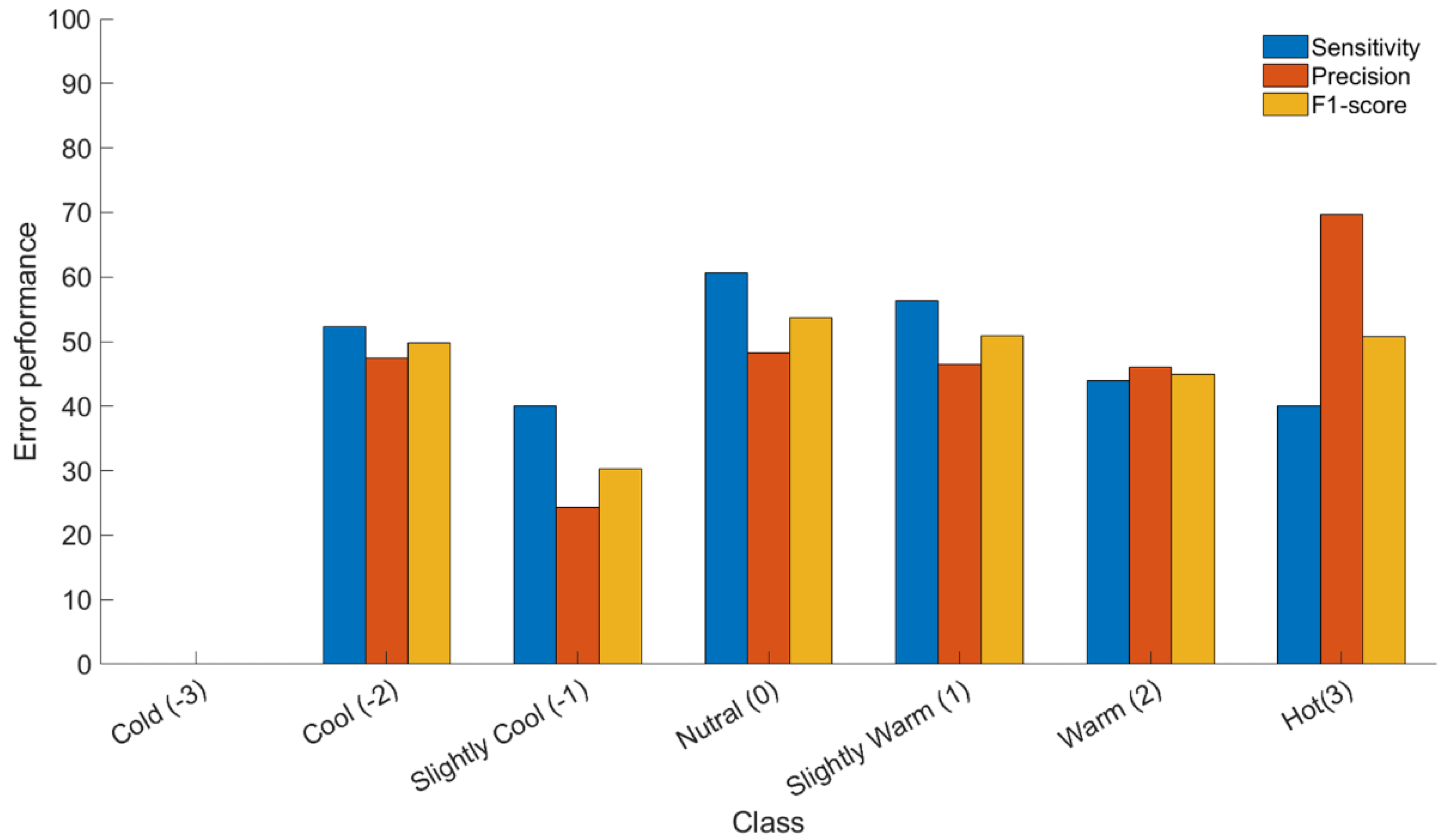
where the value of each cell $\left(i,j\right)$ represents the number of times (as percentage ‘%’) that class $j$ is classified as class $i$. Given that the optimal situation is $100\text{\%}$ for $i=j$. From the resulted confusion matrix (Table 4) the overall accuracy of the developed classifier (Model I) is calculated to be 51%. In Table 4, there is the prediction result noted as ‘Else’, which represents the case that the classifier could not assign the test point to any of the presented classes. The error performance of the developed general model is depicted in Figure 5.

3.1.2. Developing a General Model for 7-Classes Classification Problem with Dimension Reduction (Model II)

As shown in Table 3, the input space of Model I included all extracted features (54 features) that were obtained from the measured variables. However, for the sake of the main objective of the present work, the computational cost of the developed algorithm should be low enough to be compatible with wearable technology and online modeling. Hence, a feature selection procedure was employed to obtain the most reduced-dimension input space for the classification model yet with the best error performance. Feature selection here is based on evaluating all possible feature combinations and selecting the combination with best error performance. The used feature selection procedure resulted in a reduced input space of only 12 features with optimal feature combination. The selected features comprise: gender, age, $H_{R }$, $T_{er }$, $T_{sk }$, $\Delta \overline{T}$, ${\overline{q}}_{sk}$, $rms$ ($H_{r }$, $T_{c }$, $T_{sk }$, $\dot{q}$), and $\frac{d\dot{{\overline{q}}_{sk}}}{dt}$ (time-derivative of average heat flux). The feature selection step reduced the input space from 54 features to only 12, which effectively reduced the computational costs of the classification algorithm during online implementation.

The reduced dimension input space, including the selected 12 features, was used to develop a general classification model for the 7-classes classification problem to predict the thermal sensation of all test subjects. The resulted classification confusion matrix for the developed general model using the reduced-dimension input space is shown in

Table 5. The normalized confusion matrix of Model II.

		$\mathbf{Actual}\mathbf{Label}\left(\mathit{i}\right)$
		Cold %	Cool %	Slightly Cool %	Neutral %	Slightly Warm%	Warm %	Hot %
Prediction label ($\mathit{j}$)	Else	0	4.79	6.65	0	10.40	16.03	0
	Cold	0	0	0	0	0	0	0
	Cool	33.20	33.33	0	0	0	0	0
	Slightly cool	66.80	57.08	66.69	8.45	2.10	0	0
	Neutral	0	4.79	26.66	71.81	22.90	4.03	0
	Slightly Warm	0	0	0	18.32	56.25	31.96	6.71
	Warm	0	0	0	1.42	8.35	35.99	46.65
	Hot	0	0	0	0	0	12.00	46.65

. The results showed an overall accuracy of the developed classification model of 57% with an improvement of 6% compared to the results of model I. The overall error performance (sensitively, precision and F1-score) results are shown in Figure 6.

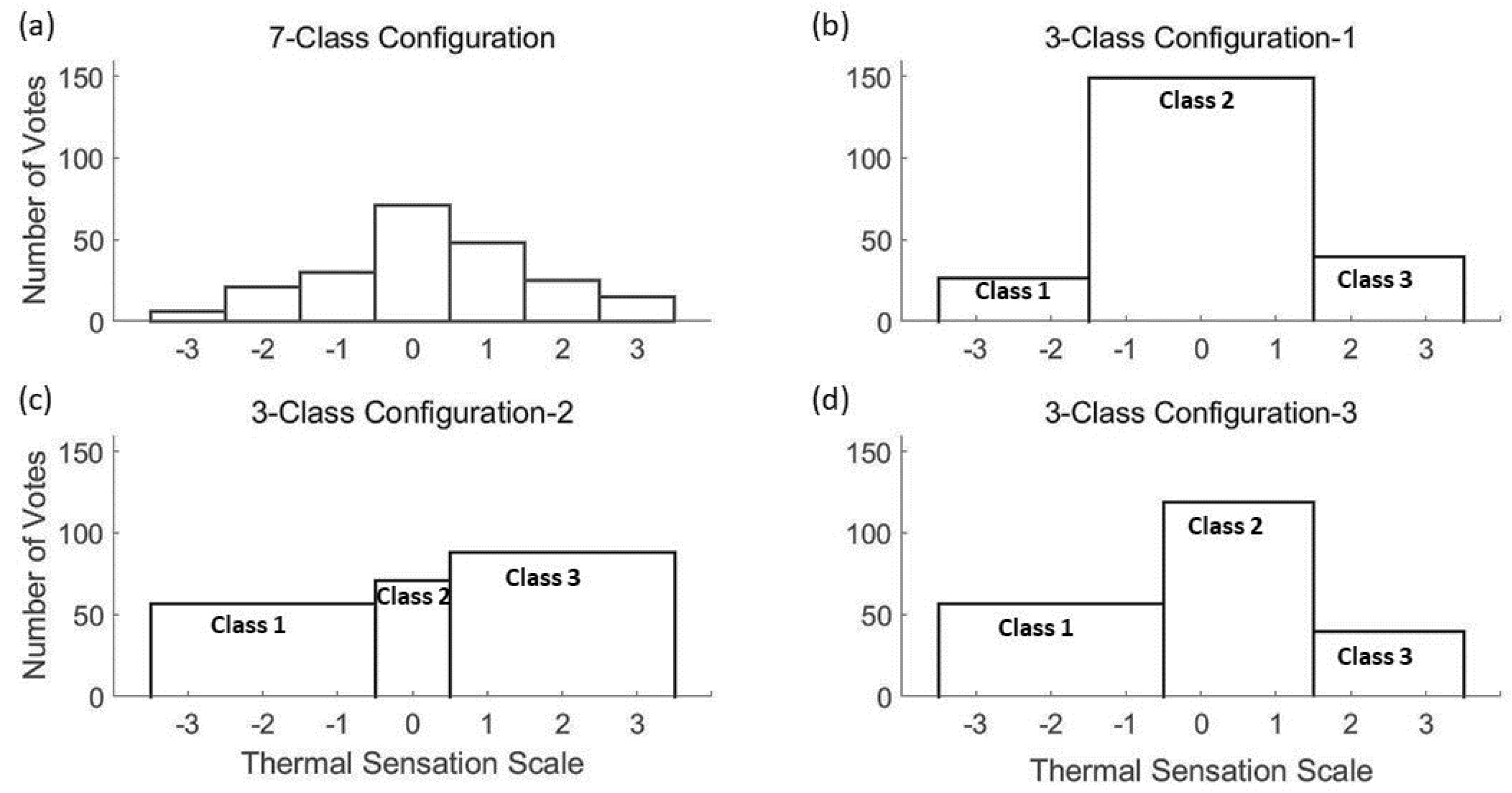
3.2. Class Reduction

From the confusion matrix in Table 5, it can be seen that the confusion is mostly observed between the adjacent classes. The main reason of such interclass confusion is that the features are not able to discriminate completely between these adjacent classes. For instance, the actual neutral class (0) is confused with 8.45% and 18.32% with slightly cool (−1) and slightly warm (1) classes, respectively. Hence, it is more convenient to reduce the seven thermal sensation classes into three classes representing thermal comfort (comfortable, uncomfortably cool, and uncomfortably warm). The class reduction is done based on three criteria, namely, maximum confusion, acceptable class imbalance, and avoiding overlap between classes. As mentioned earlier, the maximum confusion is observed between the adjacent classes (see Table 5). However, it is not possible to merge all adjacent confused classes due to the overlap. For example, the Slightly-Warm class is confused with the Neutral class by 22.9%, on the other hand, the Warm class is confused with the Slightly-warm by 31.96%. Hence, in order to merge the Slightly-warm class with the Neutral it should not be merged with Warm and vice versa. Therefore, merging must avoid any overlap between different classes. Another criterion is the class imbalance, as shown in Figure 7a and Table 5, where Cold is not recognized by the classifier due to the relatively very low number of instances labeled as Cold compared to the other classes. For an acceptable class imbalance, it is meant to consider the already existing class imbalance between the whole states that the frequency of a state occurrence is reducing by moving far from the Neutral state, as shown in Figure 7a.

Finally, it is necessary to avoid any overlap between the reduced classes by assigning each state to only one class. As there are different possibilities to obtain the new three classes, it is found that three configurations are the closest to the thermal comfort levels, considering the earlier mentioned criteria. Based on these criteria the seven classes were reduced into three classes with three different configurations as follows:

• Configuration 1 Merging the states of Cold (−3) and Cool (−2) into ‘Class 1’ (27 instances), merging Slightly cool (−1), Neutral (0), and Slightly warm (1) into ‘Class 2’ (149 instances), and merging Warm (2) and Hot (3) into ‘Class 3’ (40 instances) (Figure 7b).
• Configuration 2 Merging the states of Cold, Cool and Slightly-cool into ‘Class 1’ (57 instances), Neutral as ‘Class 2’ (71), and merging Slightly-warm, warm and Hot into ‘Class 3’ (88 instances) (Figure 7c).
• Configuration 3 Merging the states of Cold, Cool and Slightly-cool into ‘Class 1’ (57 instances), merging Neutral, and Slightly-warm into ‘Class 2’ (119 instances), and merging warm and Hot into ‘Class 3’ (40 instances) (Figure 7d).

As shown in Figure 7, each configuration has a different class distribution (i.e., number of instances per class).

Developing General Models with the Selected Features for 3-Classes Problem with Different Class Configurations (Model III)

The error performance results of the developed classification model (Model III), based on the 12 selected features, for the three labelling configurations (Conf. 1, Conf. 2 and Conf. 3) are shown in

Table 6. The error performance (precision, sensitivity, F1-score, and accuracy) of general Least Squares Support Vector Machine (LS-SVM) model for the three different 3-class configurations.

Configurations	Classes	Precision	Sensitivity	F1-Score	Accuracy
Conf. 1	Class 1	0.53	0.37	0.44	0.81
	Class 2	0.83	0.89	0.86
	Class 3	0.79	0.75	0.77
Conf. 2	Class 1	0.88	0.88	0.88	0.81
	Class 2	0.75	0.66	0.70
	Class 3	0.82	0.89	0.86
Conf. 3	Class 1	0.88	0.88	0.88	0.85
	Class 2	0.88	0.91	0.89
	Class 3	0.88	0.78	0.83

. Comparing the three configurations is not consistent, as for each configuration, the number of data-pointdata-points change, which influences the performance especially for such small size dataset.

3.3. Personalized Classification Models

In order to develop online-personalized models, it is necessary to consider two main challenges, first the developed model should be able to handle the new, personal, data in the training set. Additionally, the developed model should be adapted to the new personal data without any bias to the majority of the old (non-personal) data. Different approaches are used to handle these challenges such as incremental learning methods [34], which work on adapting and retuning the parameters of the general model based on the newly collected data. Another approach is the localized learning, which is based on developing a local model for each test point or subset of the test set [35]. In the present paper, the KNN-LS-SVM localized learning approach is used because of its simplicity and efficiency. Two techniques were used to test the localized models, the first based on LOSO testing approach, and the second approach was based on leave-one-out (LOO) testing approach.

3.3.1. Developing Personalized Models Using the Selected 12 Features and Different Class-Configurations Based on LOSO Testing Approach

As explained earlier, to develop a personalized classification model the new personal data were not considered in the training set to compare the performance with the global model. In other words, the new subject (the subject data that left out of the training set) is completely unknown to the model, which simulates the case when the model is dealing with an unknown test subject. The used localized learning approach of KNN-LS-SVM searches for the most similar (based on the similarity criterion, see (3)) training points to the new test point (from the new subject) in the input space by which a local model is developed to classify this test point. The resulted error performance (precision, sensitivity, F1-score, and accuracy) of the KNN-LS-SVM classifier based on LOSO testing approach and $K$ = 5 is presented in

Table 7. The error performance (precision, sensitivity, F1-score, and accuracy) of the localized model KNN-LS-SVM model for the three different 3-class configurations based on leave-one-subject-out (LOSO) testing approach.

Configurations	Classes	Precision	Sensitivity	F1-Score	Accuracy
Conf. 1	Class 1	0.47	0.36	0.41	0.83
	Class 2	0.84	0.90	0.87
	Class 3	0.83	0.71	0.77
Conf. 2	Class 1	0.84	0.95	0.89	0.81
	Class 2	0.74	0.68	0.70
	Class 3	0.84	0.83	0.83
Conf. 3	Class 1	0.87	0.94	0.90	0.85
	Class 2	0.88	0.89	0.88
	Class 3	0.86	0.74	0.79

.

3.3.2. Developing Personalized Models Using the Selected 12 Features and Different Class-Configurations Based on Leave-One-Out (LOO) Approach

In contrast with the first approach, for each subject one data-point is tested and the rest of the same subject data-pointdata-points are integrated with the training data. This approach mimics online personalized streaming modelling, since the new streaming personal data is considered in the training dataset and a dedicated classifier is developed online for each new test data-point. The obtained error performance of the KNN-LS-SVM classifier based on LOO testing approach and K = 5 is depicted in

Table 8. The error performance (precision, sensitivity, F1-score, and accuracy) of the localized model KNN-LS-SVM model for the three different 3-class configurations based on leave-one-out (LOO) testing approach.

Configurations	Classes	Precision	Sensitivity	F1-Score	Accuracy
Conf. 1	Class 1	0.75	0.56	0.64	0.86
	Class 2	0.87	0.93 *	0.90 *
	Class 3	0.86	0.78	0.82
Conf. 2	Class 1	0.84 *	0.95 *	0.89 *	0.79
	Class 2	0.71	0.62	0.66
	Class 3	0.81	0.83 *	0.82
Conf. 3	Class 1	0.84 *	0.91	0.87	0.87 *
	Class 2	0.89 *	0.88	0.88
	Class 3	0.89 *	0.80	0.84 *

* indicates the highest error performance value for each class in the different configurations.

.

For the proposed personalized models, the first approach of LOSO is mimicking the case that the model is applied to an unknown subject to predict individual’s thermal sensation level based on the measured variables. The localized model is searching for the most similar (nearest) training points to each test point, of this subject, that to train the classification model for each test point. This approach could be useful in case of having a large amount of data with a diversity of subjects especially in the absence of streaming data from new subjects. The second approach of LOO mimics the case of having a prior knowledge about the test subject through personally labelled data. The localized model in this approach is also searching for the most similar training points, which may include this subject personal data. This approach can be efficient in the presence of streaming personal data that is labelled by the test subject.

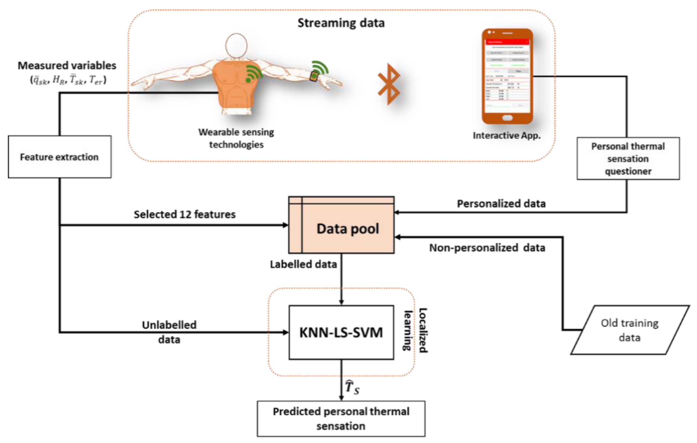
3.4. Streaming Algorithm Approach for Personalized Thermal Sensation Monitoring

In this paper, we introduce the main framework of streaming algorithm for personalized classification model to predict individual’s thermal sensation based on streaming data obtained from wearable sensors. The main framework of the proposed streaming algorithm approach is depicted in Figure 8.

The main components of the proposed algorithm (Figure 8) are explained in the following:

- Streaming data

The availability of the real-time sensors data, from the wearable technologies, has given the possibility of streaming data, which processed via the proposed online streaming algorithm to adapt and personalize the classifier model. The streaming data includes:

I.

Wearable sensor data, which consists of the continuously measured variables, namely, individual’s heart rate, skin heat flux, skin temperature, ambient temperature and aural temperature.

II.

Data obtained from the interactive mobile App., which consists of personal data, namely, age and gender. Additionally, the individual’s thermal sensation vote is to be obtained via mobile application-based questioner.

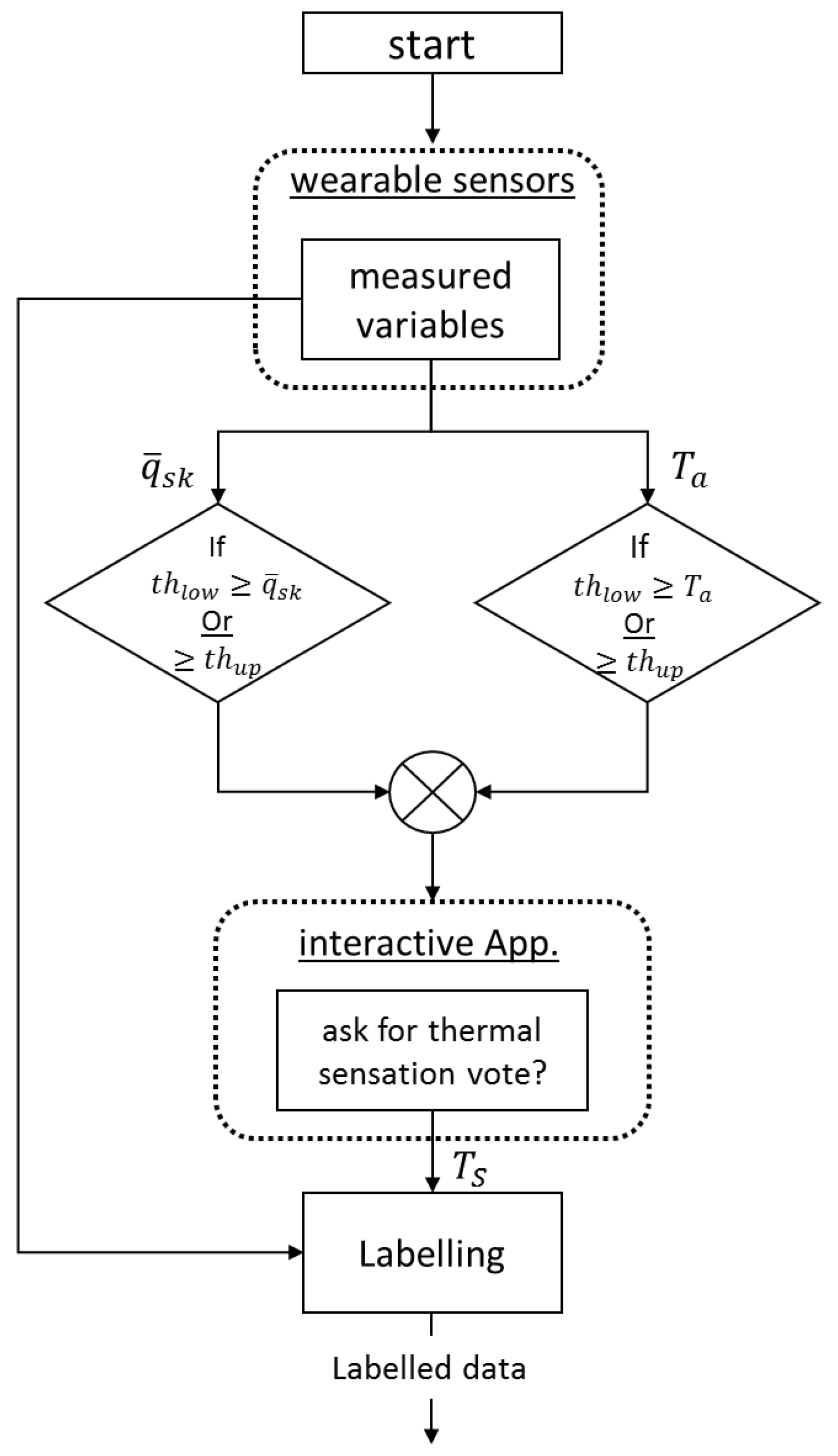
The workflow procedures of streaming data acquisition and labelling are depicted by the flowchart shown in Figure 9.

- Feature extraction

As shown earlier, the selected 12 features are extracted from the continuously measured variables, namely, $H_{R }$, $T_{er }$, $T_{sk }$, $\Delta \overline{T}$, ${\overline{q}}_{sk}$, the $rms$ of ($H_{r }$, $T_{c }$, $T_{sk }$, $\dot{q}$), and $\frac{d\dot{{\overline{q}}_{sk}}}{dt}$. Other personal futures, namely, age and gender are to be obtained via the interactive mobile App. from individual users.

- Labelled data

All training data must be labelled, either the old training data or the new personal data. Personal data is labelled manually via the questionnaire provided by the mobile App.

- Unlabelled data

Unlabelled data is the new data points to be labelled by the classifier, these unlabelled data points include the extracted features from the measured variables.

- Localized Learning Algorithm

The localized learning algorithm (i.e., KNN-LS-SVM) is the classifier that receives the unlabelled data points and train a dedicated model with the $K$ nearest training points in order to label the unlabelled ones. The output of this process is a predicted label of personal thermal sensation (${\widehat{T}}_S$).

4. Discussion

The main advantage of the proposed classification model in the present work, in comparison with other proposed models in recent studies (e.g., [17,22,25,28]), is its capability to handle the requirements for adaptive personalization and online streaming modelling. Moreover, the proposed model is reduced-dimension, with the minimum possible number of features, which makes it computationally suitable for smart wearable technologies.

The main results and findings of the present study is compared with recent studies that treat the prediction of the thermal sensation/comfort as a classification problem using machine-learning techniques.

In their study [27], Ghahramani et al. used HMM classification technique, in which three classes of thermal comfort, namely, comfortable, uncomfortably cool and uncomfortably warm are used. An important point to be considered in the work of Ghahramani et al. [27] is the class imbalance in their used experimental data between the positive class (comfortable), which represents 81% of the data and the negative class (uncomfortable), which represents only 19% of the data. Therefore, using the classification accuracy (reported 82.8 %) is considered misleading in this case. Hence, it is much more suitable in their case to compare the precision and sensitivity of this model and our general model (Model III Conf. 3). The reported results [27] of Ghahramani et al. showed a precision of 93.3% and sensitivity of 56.22% without clarifying the precision and sensitivity of the uncomfortable states of warm and cool. On the other hand, our results of (Model III Conf. 3), which is the closest to the compared approach, show a precision of 88% for all classes and sensitivity of 88%, 91%, and 78% for Class 1, Class 2, and Class 3, respectively. These results show more balance between precision and sensitivity for each class. Moreover, personalization and streaming algorithm compatibility is missing in their study.

Another relevant study [28], by Jiang et al., attempted to develop a personalized classification model, as for each subject, a classification model is trained with 50% of that subject data and tested with the rest. The reported result of this study [28] showed an average accuracy over all subjects of 89.82%. However, there is no clarification of the class distribution; hence, it is not clear whether the accuracy is efficient enough for evaluation. Moreover, it is not consistent to compare our final personalized model with that model as the latter is learned with seven classes; however, the former is learned with three classes.

In another comparable study [25] to our present work, Farhan et al., predicted individual thermal comfort using machine learning classifier. In their study Farhan et al., used publicly available dataset from which a balanced number of each class is chosen to train and test the classification model. Their developed classification model is trained with three classes that represent the three thermal comfort states of uncomfortably cool, neutral and uncomfortably warm divided based on predefined comfort thresholds. In contrast to our proposed classification model, the proposed classifiers in [25] do not consider model personalization or streaming online modelling. The best-obtained results amongst their developed models are of the SVM classifier as follows: precisions of (76.92, 62.8, and 94.2%) and sensitivities of (67.5, 89.8, and 75.7%) for classes −1, 0, and 1 respectively. On the other hand, our obtained results of (Model III conf. 3) are precisions of (88, 88, and 88%) and sensitivities of (88, 91, and 78%) of classes 1, 2, and 3 respectively. It is observed that the precisions of our developed classification model are more consistent for all classes, and the sensitivities are higher in total. Ultimately, their approach [25] does not consider personalizing the model or streaming online modelling.

In another recent study [17], a personal model is discussed; however, it is strictly applied to two subjects (male and female), unlike the case in the present study where we test the model on 25 test subjects.

After comparing our methodology and results with number of relevant and comparable studies, it is obvious that the presented study tackled number of classification and modeling challenges unlike many of the aforementioned relevant works. These challenges included the feature selection and dimension reduction, considering new streaming personal data into the training set with keeping the model complexity, rigidness against the problem of class imbalance, and ultimately personalizing the classification model using easily measured variable obtained from wearable sensors.

5. Conclusions

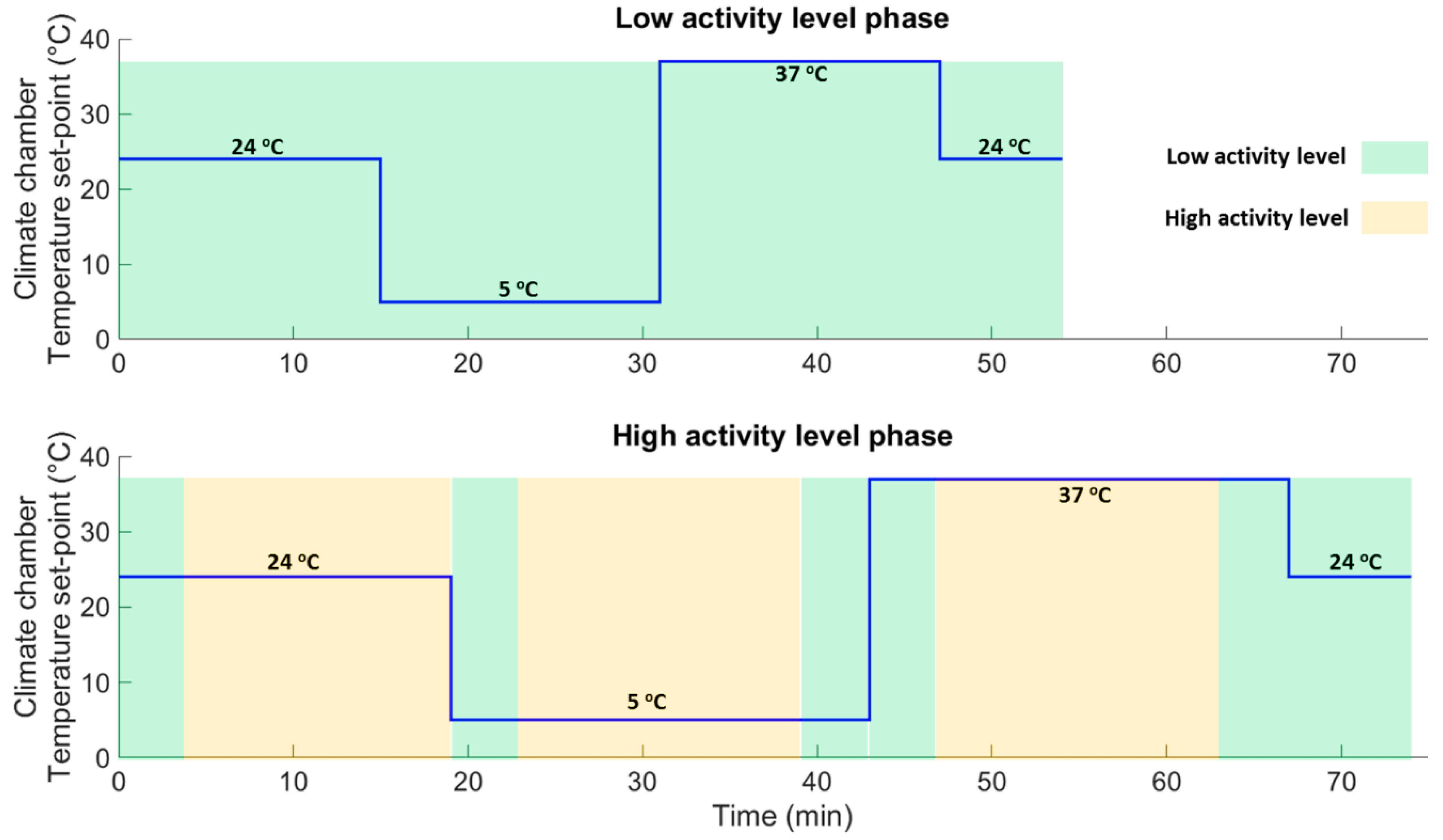
In this present paper, 25 participants are subjected to three different environmental temperatures, namely 5 °C (cold), 20 °C (moderate) and 37 °C (hot) at two different activity levels, namely, at low level (rest) and high level (cycling at 80 W power). Metabolic rate, heart rate, average skin temperature (from three different body locations), heat flux and aural temperature are measured continuously during the course of the experiments. The thermal sensation votes are collected from each test subject based on ASHRAE 7-points questioner. A general classification model based on LS-SVM technique is developed to predict the individual’s thermal sensation. A localized learning algorithm based on KNN-LS-SVM approach is used to develop a personalized classification model to predict the individual’s thermal sensation for 3-classes classification model. The developed classification model has the advantage of using a reduced-dimension input-space, which is suitable for wearable applications and online streaming algorithm. The developed personalized model showed an overall accuracy result of 86%. Additionally, we introduced the main framework of streaming algorithm based on the developed personalized classification model to predict individual’s thermal sensation based on streaming data obtained from wearable sensors. In the present work, we believe that it is the first time to utilize the localized learning approach in the thermal state classification problem. One of the main advantages of the proposed approach, in this paper, that it is suitable for streaming algorithm and online modelling as the computational cost is not influenced by increasing the number of data-points. However, the newly obtained data-points is to be considered to develop the online model, which is the main advantage of the KNN-LSSVM. Furthermore, the localized learning approach enables personalization of the classification model by considering either the personally labelled data-points or the most similar data-points of other persons. On the other hand, number of limitations, concerning the developed model, should be acknowledged here. One important limitation to the developed classification model is regarding to the data size, as the number of data-points per person and in total are generally limited. Moreover, the 7-classes labeling is unbalanced, which made the class reduction is necessary to enhance the overall prediction performance during the course of this study. Otherwise, this study would be extended to be applied to a 7-classes classification problem. The data balance and data size can be enhanced by asking for more frequent votes during the experiment and considering more than three environment temperature levels. Finally, another limitation regards the proposed KNN-LSSVM modeling approach, in which an extra hyperparameter (i.e., $K$) is to be optimized, which adds an extra computational cost to the overall streaming algorithm.

References

1. ASHRAE. Thermal Environmental Conditions for Human Occupancy; American Society of Heating, Refrigeration and Air Conditioning Engineers, Inc.: Atlanta, GA, USA, 2004. [Google Scholar]
2. ISO-10551. Ergonomics of the Thermal Environmen—Assessment of the Influence of the Thermal Environment Using Subjective Judgement Scales; ISO: Brussels, Belgium, 1995. [Google Scholar]
3. Fanger, P.O. Thermal Comfort: Analysis and Applications In Environmental Engineering, 1st ed.; Danish Technical Press: Lyngby, Denmark, 1970. [Google Scholar]
4. Koelblen, B.; Psikuta, A.; Bogdan, A.; Annaheim, S.; Rossi, R.M. Thermal sensation models: A systematic comparison. Indoor Air 2017, 27, 680–689. [Google Scholar] [CrossRef] [PubMed]
5. Enescu, D. Models and Indicators to Assess Thermal Sensation Under Steady-state and Transient Conditions. Energies 2019, 12, 841. [Google Scholar] [CrossRef]
6. Kenneth, K.C.; Parsons, C. Human Thermal Environments: The Effects of Hot, Moderate and Cold Environments on Human Health, Comfort and Performance, 3rd ed.; CRC Press: Boca Raton, FL, USA, 2014. [Google Scholar]
7. Nikolopoulou, M.; Steemers, K. Thermal comfort and psychological adaptation as a guide for designing urban spaces. Energy Build. 2003, 35, 95–101. [Google Scholar] [CrossRef]
8. Gagge, A.P.; Stolwijk, J.A.J.; Nishi, Y. An Effective Temperature Scale Based on a Simple Model of Human Physiological Regulatory Response. ASHRAE Trans. 1971, 77, 247–262. [Google Scholar]
9. Takada, S.; Matsumoto, S.; Matsushita, T. Prediction of whole-body thermal sensation in the non-steady state based on skin temperature. Build. Environ. 2013, 68, 123–133. [Google Scholar] [CrossRef]
10. Fiala, D. Dynamic Simulation of Human Heat Transfer and Thermal Comfort; De Montfort University: Leicester, UK, 1998. [Google Scholar]
11. Lomas, K.J.; Fiala, D.; Stohrer, M. First principles modeling of thermal sensation responses in steady-state and transient conditions. ASHRAE Trans. 2003, 109, 179–186. [Google Scholar]
12. Zhang, H. Human Thermal Sensation and Comfort in Transient and Non-Uniform Thermal Environments; University of California, Berkeley: Berkeley, CA, USA, 2003. [Google Scholar]
13. Guan, Y.; Hosni, M.H.; Jones, B.W.; Gielda, T.P. Investigation of Human Thermal Comfort Under Highly Transient Conditions for Automotive Applications-Part 2: Thermal Sensation Modeling. ASHRAE Trans. 2003, 109, 898–907. [Google Scholar]
14. Guan, Y.; Hosni, M.H.; Jones, B.W.; Gielda, T.P. Investigation of Human Thermal Comfort Under Highly Transient Conditions for Automotive Applications-Part 1: Experimental Design and Human Subject Testing Implementation. ASHRAE Trans. 2003, 109, 885–897. [Google Scholar]
15. Nilsson, H.O.; Holmer, I. Comfort climate evaluation with thermal manikin methods and computer simulation models. Indoor Air 2003, 13, 28–37. [Google Scholar] [CrossRef] [PubMed]
16. Kingma, B.R.M.; Schellen, L.; Frijns, A.J.H.; Lichtenbelt, W.D.V. Thermal sensation: A mathematical model based on neurophysiology. Indoor Air 2012, 22, 253–262. [Google Scholar] [CrossRef] [PubMed]
17. Lu, S.; Wang, W.; Wang, S.; Hameen, E.C. Thermal Comfort-Based Personalized Models with Non-Intrusive Sensing Technique in Office Buildings. Appl. Sci. 2019, 9, 1768. [Google Scholar] [CrossRef]
18. de Dear, R.; Brager, G.S. Developing an adaptive model of thermal comfort and preference. ASHRAE Trans. 1998, 104, 145–167. [Google Scholar]
19. Rijal, H.B.; Gumphreys, M.; Tuohy, P.; Nicol, F. Development of adaptive algorithms for the operation of windows, fans and doors to predict thermal comfort and energy use in Pakistani buildings. ASHRAE Trans. 2008, 114, 555–573. [Google Scholar]
20. Humphreys, M. Outdoor temperatures and comfort indoors. Batim. Int. Build. Res. Pract. 1978, 6, 92. [Google Scholar] [CrossRef]
21. Lee, S.; Bilionis, I.; Karava, P.; Tzempelikos, A. A Bayesian approach for probabilistic classification and inference of occupant thermal preferences in office buildings. Build. Environ. 2017, 118, 323–343. [Google Scholar] [CrossRef] [Green Version]
22. Ghahramani, A.; Castro, G.; Karvigh, S.A.; Becerik-Gerber, B. Towards unsupervised learning of thermal comfort using infrared thermography. Appl. Energy 2018, 211, 41–49. [Google Scholar] [CrossRef] [Green Version]
23. Kim, J.; Zhou, Y.; Schiavon, S.; Raftery, P.; Brager, G. Personal comfort models: Predicting individuals’ thermal preference using occupant heating and cooling behavior and machine learning. Build. Environ. 2018, 129, 96–106. [Google Scholar] [CrossRef]
24. Chaudhuri, T.; Soh, Y.C.; Li, H.; Xie, L. Machine learning based prediction of thermal comfort in buildings of equatorial Singapore. In Proceedings of the 2017 IEEE International Conference on Smart Grid and Smart Cities (ICSGSC), Singapore, 23–26 July 2017; pp. 72–77. [Google Scholar]
25. Farhan, A.A.; Pattipati, K.; Wang, B.; Luh, P. Predicting individual thermal comfort using machine learning algorithms. In Proceedings of the 2015 IEEE International Conference on Automation Science and Engineering (CASE), Gothenburg, Sweden, 24–28 August 2015; pp. 708–713. [Google Scholar]
26. Dai, C.; Zhang, H.; Arens, E.; Lian, Z. Machine learning approaches to predict thermal demands using skin temperatures: Steady-state conditions. Build. Environ. 2017, 114, 1–10. [Google Scholar] [CrossRef] [Green Version]
27. Huang, C.C.; Yang, R.; Newman, M.W. The potential and challenges of inferring thermal comfort at home using commodity sensors. In Proceedings of the 2015 ACM International Joint Conference on Pervasive and Ubiquitous Computing, Osaka, Japan, 7–11 September 2015; pp. 1089–1100. [Google Scholar]
28. Jiang, L.; Yao, R. Modelling personal thermal sensations using C-Support Vector Classification (C-SVC) algorithm. Build. Environ. 2016, 99, 98–106. [Google Scholar] [CrossRef] [Green Version]
29. Hussain, S.; Kang, B.H.; Lee, S. A Wearable Device-Based Personalized Big Data Analysis Model. In Lecture Notes in Computer Science; Springer: Cham, Swizterland, 2014; Volume 8867, pp. 236–242. [Google Scholar]
30. Suykens, J.A.K.; van Gestel, T.; de Brabanter, J.; de Moor, B.; Vandewalle, J. Least Squares Support Vector Machine; World Scientific: Singapore, 2002. [Google Scholar]
31. Amer, A.Y.A. Localized Least Squares Support Vector Machines with Application to Weather Forecasting; KU Leuven: Leuven, Belgium, 2016. [Google Scholar]
32. Ashrae, Ashrae Standard 55; American Society of Heating, Refrigerating and Air-Conditioning Engineers Inc.: Atlanta, GA, USA, 2017.
33. Dewhirst, M.W.; Viglianti, B.L.; Lora-Michiels, M.; Hanson, M.; Hoopes, P.J. Basic principles of thermal dosimetry and thermal thresholds for tissue damage from hyperthermia. Int. J. Hyperth 2003, 19, 267–294. [Google Scholar] [CrossRef]
34. Losing, V.; Hammer, B.; Wersing, H. Incremental on-line learning: A review and comparison of state of the art algorithms. Neurocomputing 2018, 275, 1261–1274. [Google Scholar] [CrossRef] [Green Version]
35. Bottou, L.; Vepnik, V. Local learning algorithms. Neural Comput. 1992, 4, 888–900. [Google Scholar] [CrossRef]
Figure 1. A flow chart illustrating the algorithm of K-Nearest Neighbours Least Squares Support Vector Machines (KNN-LS-SVM) classifier.
Applsci 09 03303 g001
Figure 2. Photographic picture of the three climate-controlled rooms (from right to left, A–C).
Applsci 09 03303 g002
Figure 3. Sensor placement. (A) Ear channel for aural temperature measurement via the Cosinuss One, (B) upper arm where skin temperature and heat flux are measured with the gSKIN patch, (C) middle upper chest where skin temperature and heat flux are measured with the gSKIN patch, (D) lower chest where heart rate is measured with the Polar H7, (E) Scapula where skin temperature is measured with the shimmer, (F) mouth and nose where metabolic rate is measured via the MetaMAX-3B spiroergometer sensor.
Applsci 09 03303 g003
Figure 4. Plots showing the climate chambers’ set-point temperatures programmed during the 55 min low activity phase (upper graph) and the 75 min high activity phase (lower graph).
Applsci 09 03303 g004
Figure 5. Error performance of the developed general classification model with 54 input features for 7-classes classification problem.
Applsci 09 03303 g005
Figure 6. Error performance of the developed general classification model with the selected 12 input features (reduced dimension input space) for 7-classes classification problem.
Applsci 09 03303 g006
Figure 7. (a) A histogram of 7-class thermal sensation scale of ASHRAE system. (b) A histogram of 3-class thermal sensation of Configuration 1. (c) A histogram of 3-class thermal sensation of Configuration 2. (d) A histogram of 3-class of Configuration 3.
Applsci 09 03303 g007
Figure 8. Schematic representation of the proposed streaming algorithm for online personalized thermal sensation monitoring.
Applsci 09 03303 g008
Figure 9. Flowchart represents the main workflow of the streaming data acquisition and labeling process.
Applsci 09 03303 g009