Form-Finding Analysis of a Class 2 Tensegrity Robot

Abstract

In this paper, a new form-finding analysis methodology for a class 2 tensegrity robot is proposed. The methodology consists of two steps: first, the analysis of the possible geometric configurations of the robot is carried out through the results of the kinematic position analysis; and, second, from the static analysis, the equilibrium positions of the robot are found, which represents its workspace. Both kinematics and static analysis are resolved in a closed-form using basic tools of linear algebra instead of the strategies used in literature. Four numerical experiments are presented using the finite element analysis software ANSYS^©. Additionally, a comparison between the results of the form-finding analysis methodology proposed and the ANSYS^© results is presented.

1. Introduction

A tensegrity system is established when a discontinuous set of compression components interacts with a continuous set of tension components to define a stable volume in space [1]. The biggest advantage of tensegrity systems is their low weight and high stiffness, which makes them particularly good for many applications from architecture to robotics. It should be mentioned that the components of tensegrity systems are subject only to axial loads.

Due to their characteristics, tensegrities can be considered as biomimetic structures and have shown the capability to create lightweight, strong and fault tolerant robots with latent potential for applications such as a spine-like tensegrity moving robot [2] and a bio-inspired tensegrity manipulator [3], which resembles the biomechanics of a human arm. Researchers consider this as an opportunity to include tensegrity robots in the field of soft robotics due to their biological inspiration and inherent ability to combine stiff elements with soft materials to create deformable robots [4,5]. Some examples found in the literature are the soft robotic muscle by Xiang et al. [6] and the soft robotic system by Cheng et al. [7], both of which use a combination of springs and electric muscles to modify their shape.

There exists a way to distinguish between various types of tensegrity systems that fit in the general tensegrity definition established by Skelton and Oliveira: “A tensegrity configuration that has no contacts between its rigid bodies is a class 1 tensegrity system, and a tensegrity system with as many as k rigid bodies in contact is a class k tensegrity system” [8].

Tensegrity prisms are the simplest topological family of tensegrity systems where the basic arrangement consists of two equal polygons in parallel planes joined by members at their vertices; the polygons do not necessarily have to keep the same size or remain in parallel planes [9]. However, if it is assumed that the shapes of the upper and lower polygons do not change, platforms can be coupled at the end of the system. As a result, this device is a parallel device [10].

The structure proposed by Manríquez et al. [11] possesses these characteristics, including a system of combined flexible elements formed by a spring attached to a cable with a fixed length, where the length of its cables can be adjusted using a system of pulleys coupled to two servomotors. This mechanism was used as a case study, giving continuity to previous work where the study of the kinematic analysis of the mechanism’s position was obtained using the geometric parameters of Denavit–Hartenberg.

These new type of robots cannot be studied in the same way as conventional manipulators; new strategies for their analyses are being proposed. For example, Hao et al. [12] presented a mechanism composed of four pneumatic muscles, and they obtained its kinematic analysis with geometric parameters. Greer et al. [13] presented a mechanism that combines pneumatic muscle, a spring and a wire, the motion of which is similar to that presented in [6], and its kinematic analysis is based on geometric parameters and arc length. Regarding the kinematic analysis of tensegrity mechanisms, due to the presence of flexible components, its kinematics has been treated differently. In conventional mechanisms, kinematics includes only the geometric properties of motion. The joint variables of the mechanism are related to the position and orientation of the end-effector and these relationships are the points of interest in the study of mechanisms kinematics. By definition, in tensegrity systems, the equilibrium configuration must be maintained by the effect of the internal forces of the arrangement of its components. Therefore, various authors, e.g., Arsenault and Gosselin [14] and Shekarforoush et al. [15], considered that, in tensegrity mechanisms, the static and kinematic analysis must be considered simultaneously. The aforementioned implies that they establish the kinematic relationships of the mechanism based on the equations of static equilibrium.

In [15], Shekarforoush et al. presented two types of kinematic analysis. In the first one, the analysis is performed independently, and the results are adjusted to meet the conditions of static equilibrium. The second does not consider external loads applied to the mechanism, the static equations are found from minimizing the potential energy of the mechanism, and the kinematic analysis is derived from the static analysis.

For a complete analysis, tensegrities require a form-finding procedure, which typically requires computing a critical parameter such as a twisting angle, a cable-to-strut ratio or a force-to-length ratio [16].

Within the literature, there are different methodologies focused on the calculation of the critical parameters above mentioned. Among them, there is the algorithm proposed by Pagitz et al. [17] to find the form of a tensegrity structure, based on the theory of finite elements. Other authors used solution search strategies based on genetic algorithms, e.g., Faroughi et al. [18], and Koohestani [19], the latter of whom used genetic algorithms to transform the form-finding problem in a way that minimizes an evaluation function based on the force density matrix of the structure. Some other form-finding strategies found employ stochastic procedures to determine the different equilibrium configurations of a tensegrity structure, e.g., Feng et al. [20] who used a Monte-Carlo type method as a search engine for possible equilibrium configurations.

Similarly, Feng and Guo [21] presented a form-finding strategy that consists of a numerical algorithm designed to find the equilibrium position of class 1 and 2 tensegrity structures, without generating a hypothesis about the initial nodal coordinates, the lengths of the elements, the properties of the material, the symmetry of the structure or the condition of the force density matrix. Obara et al. [22] used a qualitative analysis of truss matrices, which consist of the compatibility matrix and stiffness matrix with the effect of self-equilibrated forces, established using the finite element method, to search for a 2D tensegrity form. In addition to the methods already mentioned, Bayat and Crane [23,24] proposed a form-finding method based on the geometric relationships between its elements, for a tensegrity structure in two dimensions.

In this paper, the proposed methodology for the form-finding analysis consists in performing the forward kinematic position analysis in combination with the static analysis for each of the geometrical configurations to find all states of self-equilibrium for which the internal forces can oppose to the external forces applied to the robot.

2. Kinematic Position Analysis

In this section, both the forward and inverse kinematic position analyses of the class 2 tensegrity robot are presented using the Denavit–Hartenberg parameters. The tensegrity robot used as a case of study in this study was presented in Manríquez et al. [11]. This robot is one of the few presented in the literature as a class 2 tensegrity robot, and the inspiration of its design is for biomechanical applications.

2.1. Forward Kinematic Position Analysis

Figure 1 shows the class 2 tensegrity robot, which is composed of two rigid substructures joined at one end by a universal joint, and four flexible elements at the remaining ends: two cables, ${\mathrm{C}}_1$ and ${\mathrm{C}}_2$, and two springs, ${\mathrm{r}}_1$ and ${\mathrm{r}}_2$.

To maintain this paper to be self-contained, the solution proposed by Manríquez et al. [11] is presented. This strategy consists of using the Denavit–Hartenberg parameters, contained in

Table 1. Denavit–Hartenberg parameters of the structure.

i	${\mathit{d}}_{\mathit{i}}$	${\mathit{\theta }}_{\mathit{i}}$	${\mathit{a}}_{\mathit{i}}$	${\mathit{\alpha }}_{\mathit{i}}$
	mm	rad	mm	rad
1	0	${\theta }_1$	0	$-\pi /2$
2	0	${\theta }_2$	$a_2$	$\pi /2$

, as well as the auxiliary reference frames ${\Sigma }_W$, ${\Sigma }_{M_1}$ and ${\Sigma }_{M_2}$, which represent the reference frame of the base, the cable joint ${\mathrm{C}}_1$ and the cable joint ${\mathrm{C}}_2$, respectively, shown in Figure 2.

With the geometric parameters of the robot and the reference frames, the rigid links that make up the robot are analyzed following the Denavit–Hartenberg methodology [25], resulting in the following homogeneous transformation matrices:

$$\begin{array}{ccc}\hfill {}^W{T}_0& =& \left[\begin{array}{cccc}1& 0& 0& {\mathit{l}}_1\\ 0& 1& 0& 0\\ 0& 0& 1& 0\\ 0& 0& 0& 1\end{array}\right]\hfill \end{array}$$

(1)

$$\begin{array}{ccc}\hfill {}^0{T}_1& =& \left[\begin{array}{cccc}c{\theta }_1& 0& -s{\theta }_1& 0\\ s{\theta }_1& 0& c{\theta }_1& 0\\ 0& -1& 0& 0\\ 0& 0& 0& 1\end{array}\right]\hfill \end{array}$$

(2)

$$\begin{array}{ccc}\hfill {}^1{T}_M& =& \left[\begin{array}{cccc}c{\theta }_2& 0& s{\theta }_2& a_2·c{\theta }_2\\ s{\theta }_2& 0& -c{\theta }_2& a_2·c{\theta }_2\\ 0& 1& 0& 0\\ 0& 0& 0& 1\end{array}\right]\hfill \end{array}$$

(3)

$$\begin{array}{ccc}\hfill {}^M{T}_{M_1}& =& \left[\begin{array}{cccc}1& 0& 0& 0\\ 0& 1& 0& {\mathit{l}}_2^{*}\\ 0& 0& 1& -{\mathit{l}}_2^{*}\\ 0& 0& 0& 1\end{array}\right]\hfill \end{array}$$

(4)

$$\begin{array}{ccc}\hfill {}^M{T}_{M_2}& =& \left[\begin{array}{cccc}1& 0& 0& 0\\ 0& 1& 0& -{\mathit{l}}_2^{*}\\ 0& 0& 1& {\mathit{l}}_2^{*}\\ 0& 0& 0& 1\end{array}\right]\hfill \end{array}$$

(5)

where $l_2^{*}=\frac{l_2}{2}$, $s{\theta }_i\equiv sin\left({\theta }_i\right)$ and $c{\theta }_i\equiv cos\left({\theta }_i\right)$ for $i=1,2$.

By multiplying Equations (1)–(5), the relative position and orientation of ${\Sigma }_{M_1}$ and ${\Sigma }_{M_2}$ with respect to ${\Sigma }_W$ is obtained, that is:

$$\begin{array}{ccc}\hfill {}^W{T}_{M_1}& =& {}^W{T}_0·{}^0{T}_1·{}^1{T}_M·{}^M{T}_{M_1}\hfill \end{array}$$

(6)

$$\begin{array}{ccc}\hfill {}^W{T}_{M_2}& =& {}^W{T}_0·{}^0{T}_1·{}^1{T}_M·{}^M{T}_{M_2}\hfill \end{array}$$

(7)

Then, the position of the origins of ${\Sigma }_{M_1}$ and ${\Sigma }_{M_2}$ with respect to ${\Sigma }_W$ are given by:

$$\begin{array}{ccc}\hfill {}^W{P}_{M_1}& =& \left[\begin{array}{c}c{\theta }_1·(-s{\theta }_2·{\mathit{l}}_2^{*}+a_2·c{\theta }_2)-s{\theta }_1·{\mathit{l}}_2^{*}+{\mathit{l}}_1\\ s{\theta }_1·(-s{\theta }_2·{\mathit{l}}_2^{*}+a_2·c{\theta }_2)+c{\theta }_1·{\mathit{l}}_2^{*}\\ -c{\theta }_2·{\mathit{l}}_2^{*}-a_2·s{\theta }_2\end{array}\right]\hfill \end{array}$$

(8)

$$\begin{array}{ccc}\hfill {}^W{P}_{M_2}& =& \left[\begin{array}{c}c{\theta }_1·(s{\theta }_2·{\mathit{l}}_2^{*}+a_2·c{\theta }_2)+s{\theta }_1·{\mathit{l}}_2^{*}+{\mathit{l}}_1\\ s{\theta }_1·(s{\theta }_2·{\mathit{l}}_2^{*}+a_2·c{\theta }_2)-c{\theta }_1·{\mathit{l}}_2^{*}\\ c{\theta }_2·{\mathit{l}}_2^{*}-a_2·s{\theta }_2\end{array}\right]\hfill \end{array}$$

(9)

To determine the variations in the length of the cables ${\mathrm{C}}_1$ and ${\mathrm{C}}_2$, the base points $B_1$ and $B_2$ must be defined (see Figure 2).

The points $B_1$ and $B_2$ are defined with respect to ${\Sigma }_W$, and they can be expressed as:

$$\begin{array}{ccc}\hfill {}^W{P}_{B_1}& =& {\left[\begin{array}{ccc}{B}_{1_x}& B_{1_y}& B_{1_z}\end{array}\right]}^T\hfill \end{array}$$

(10)

$$\begin{array}{ccc}\hfill {}^W{P}_{B_2}& =& {\left[\begin{array}{ccc}{B}_{2_x}& B_{2_y}& B_{2_z}\end{array}\right]}^T\hfill \end{array}$$

(11)

Using Equations (8)–(11), the lengths of ${\mathrm{C}}_1$ and ${\mathrm{C}}_2$ regarding the joint variables ${\theta }_1$ and ${\theta }_2$ are given by:

$$\begin{array}{ccc}\hfill L_{{\mathrm{C}}_1}& =& \sqrt{{(P_{M_{1_x}}-B_{1_x})}^2+{(P_{M_{1_y}}-B_{1_y})}^2+{(P_{M_{1_z}}-B_{1_z})}^2}\hfill \\ \hfill \end{array}$$

(12)

$$\begin{array}{ccc}\hfill L_{{\mathrm{C}}_2}& =& \sqrt{{(P_{M_{2_x}}-B_{2_x})}^2+{(P_{M_{2_y}}-B_{2_y})}^2+{(P_{M_{2_z}}-B_{2_z})}^2}\hfill \end{array}$$

(13)

Equations (12) and (13) allow calculating the position and orientation of the end-effector, represented by ${\Sigma }_M$ based on the cable lengths.

2.2. Inverse Kinematic Position Analysis

For the proposed class 2 tensegrity robot, the inverse kinematic position analysis consists on finding the joint variables ${\theta }_1$ and ${\theta }_2$, to determine the lengths of the cables ${\mathrm{C}}_1$ and ${\mathrm{C}}_2$ according to a desired position and orientation of reference frame ${\Sigma }_M$.

Then, the desired position and orientation of ${\Sigma }_M$ with respect to ${\Sigma }_W$ can be expressed by:

$${}^W{T}_M=\left[\begin{array}{cccc}{t}_{11}& t_{12}& t_{13}& x_m\\ t_{21}& t_{22}& t_{23}& y_m\\ t_{31}& t_{32}& t_{33}& z_m\\ 0& 0& 0& 1\end{array}\right]$$

(14)

From this, it is possible to obtain ${}^W{T}_M{=}^W{T}_0{·}^0{T}_1{·}^1{T}_M$, thus:

$${}^W{T}_M=\left[\begin{array}{cccc}c{\theta }_1·c{\theta }_2& -s{\theta }_1& c{\theta }_1·s{\theta }_2& {\mathit{l}}_1+a_2·c{\theta }_1·c{\theta }_2\\ s{\theta }_1·c{\theta }_2& c{\theta }_1& s{\theta }_1·s{\theta }_2& a_2·c{\theta }_2·s{\theta }_1\\ -s{\theta }_2& 0& c{\theta }_2& -a_2·s{\theta }_2\\ 0& 0& 0& 1\end{array}\right]$$

(15)

Furthermore, relating Equations (14) and (15), the joint variables ${\theta }_1$ and ${\theta }_2$ are obtained as:

$$\begin{array}{ccc}{\theta }_1& =& atan2\left(\frac{t_{23}}{t_{13}}\right)\end{array}$$

(16)

$$\begin{array}{ccc}{\theta }_2& =& atan2\left(\frac{-t_{31}}{t_{33}}\right)\end{array}$$

(17)

Thus, Equations (16) and (17) are the joint variables for a desired position and orientation of ${\Sigma }_M$. Then, the length of the cables ${\mathrm{C}}_1$ and ${\mathrm{C}}_2$ can be obtained using Equations (12) and (13), respectively.

3. Static Analysis

For a tensegrity robot, the kinematic position analysis does not provide sufficient conditions to determine whether the robot can adopt a particular geometric configuration. This is because tensegrity robots can only adopt geometrical configurations of equilibrium, i.e., geometric configurations in which the forces exerted by the flexible elements, only tension forces, can oppose to both the forces exerted by the rigid elements, only compression forces, and the external forces applied to the robot. Consequently, it is necessary to complement the forward position kinematic analysis with the static analysis of the robot to determine if a particular geometric configuration is a geometric configuration of equilibrium.

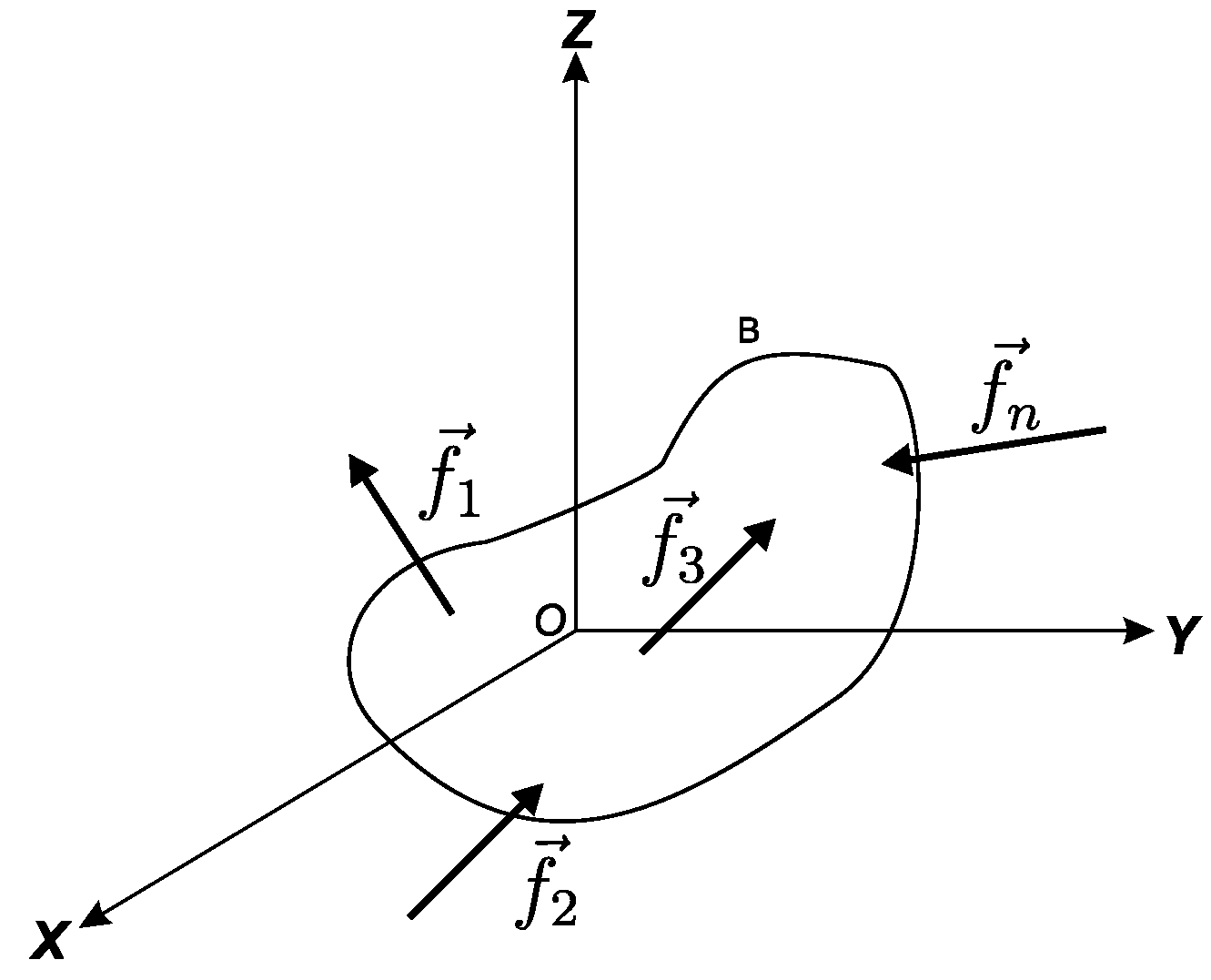
In general, if a rigid body is subjected to the action of multiple forces, $\overrightarrow{f_1},\overrightarrow{f_2},\dots ,\overrightarrow{f_n}$, as shown in Figure 3, it is possible to find an equivalent force-torque system that imprints the same physical effect on the rigid body as the original force system [26] (Figure 4).

The equivalent force, $\overrightarrow{f_e}$, and the equivalent moment, ${\overrightarrow{m}}_{e_O}$, acting on the rigid body B, are given, respectively, by:

$$\begin{array}{ccc}\hfill \overrightarrow{f_e}& =& \sum _{i=1}^n\overrightarrow{f_i}\hfill \end{array}$$

(18)

$$\begin{array}{ccc}\hfill {\overrightarrow{m}}_{e_O}& =& \sum _{i=1}^n{\overrightarrow{m}}_{O_i}\hfill \end{array}$$

(19)

If the equivalent force–torque system described in the Equations (18) and (19) equals zero, the external forces form a zero-equivalent system, and the rigid body is said to be in equilibrium. The conditions of the equilibrium above can be expressed in general terms as:

$$\begin{array}{ccc}\hfill \overrightarrow{f_e}& =& \sum _{i=1}^n\overrightarrow{f_i}=\overrightarrow{0}\hfill \end{array}$$

(20)

$$\begin{array}{ccc}\hfill {\overrightarrow{m}}_{e_O}& =& \sum _{i=1}^n{\overrightarrow{m}}_{O_i}=\overrightarrow{0}\hfill \end{array}$$

(21)

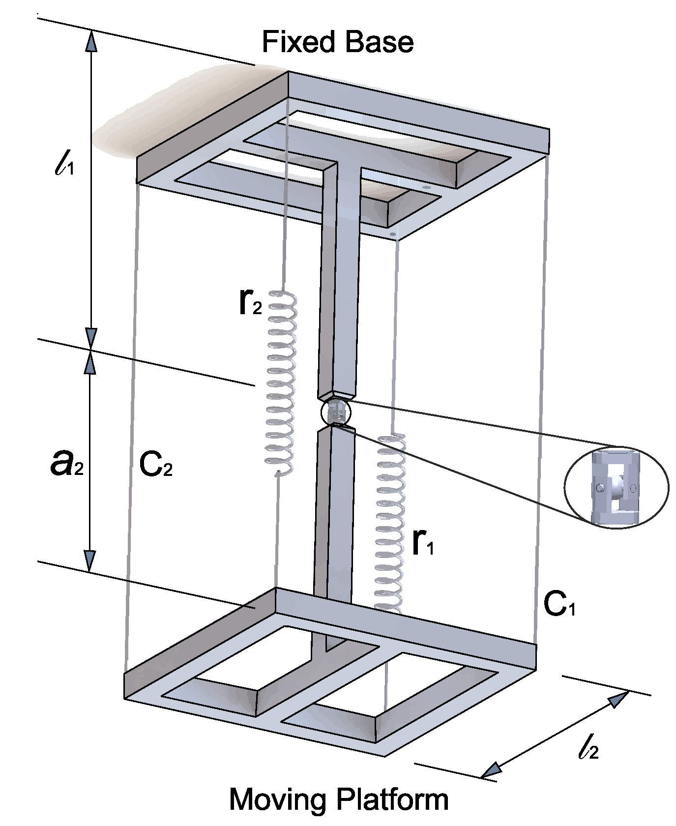
Equations (20) and (21) are taken as a basis in the development of the static analysis of the class 2 tensegrity robot. Additionally, the origin of the ${\Sigma }_0$ framework, attached to the center of the rotation axis of the first joint joined to the fixed base of the robot, is used as a point of reference for calculating displacements, forces and moments contained in the elements of the robot. Similarly, the ${\Sigma }_M$ frame, attached to the center of the moving platform, is used to describe the desired geometric configuration, i.e., the coordinates of the moving reference system as well as the lengths of the flexible elements. Additionally, it is considered that the weight of the moving platform is concentrated in the centroid, G. Based on the previous considerations, the problem of static analysis can be posed as follows:

From the forward and inverse kinematics of position analyses are obtained:

• The lengths $L_{{\mathrm{C}}_1}$ and $L_{{\mathrm{C}}_2}$ correspond to cables ${\mathrm{C}}_1$ and ${\mathrm{C}}_2$, respectively.
• The lengths $L_{{\mathrm{r}}_1}$ and $L_{{\mathrm{r}}_2}$ correspond to springs ${\mathrm{r}}_1$ and ${\mathrm{r}}_2$, respectively.
• The position and orientation of the reference frameworks ${\Sigma }_M$, ${\Sigma }_{M_1}$, ${\Sigma }_{M_2}$, ${\Sigma }_{R_1}$ and ${\Sigma }_{R_2}$ are with respect to the reference framework ${\Sigma }_W$.

Furthermore, the total mass of the robot is known.

The static analysis requires knowing the set of forces applied by the flexible elements on the moving platform to ensure that the robot is in a geometric equilibrium configuration, according to the conditions described in Equations (20) and (21).

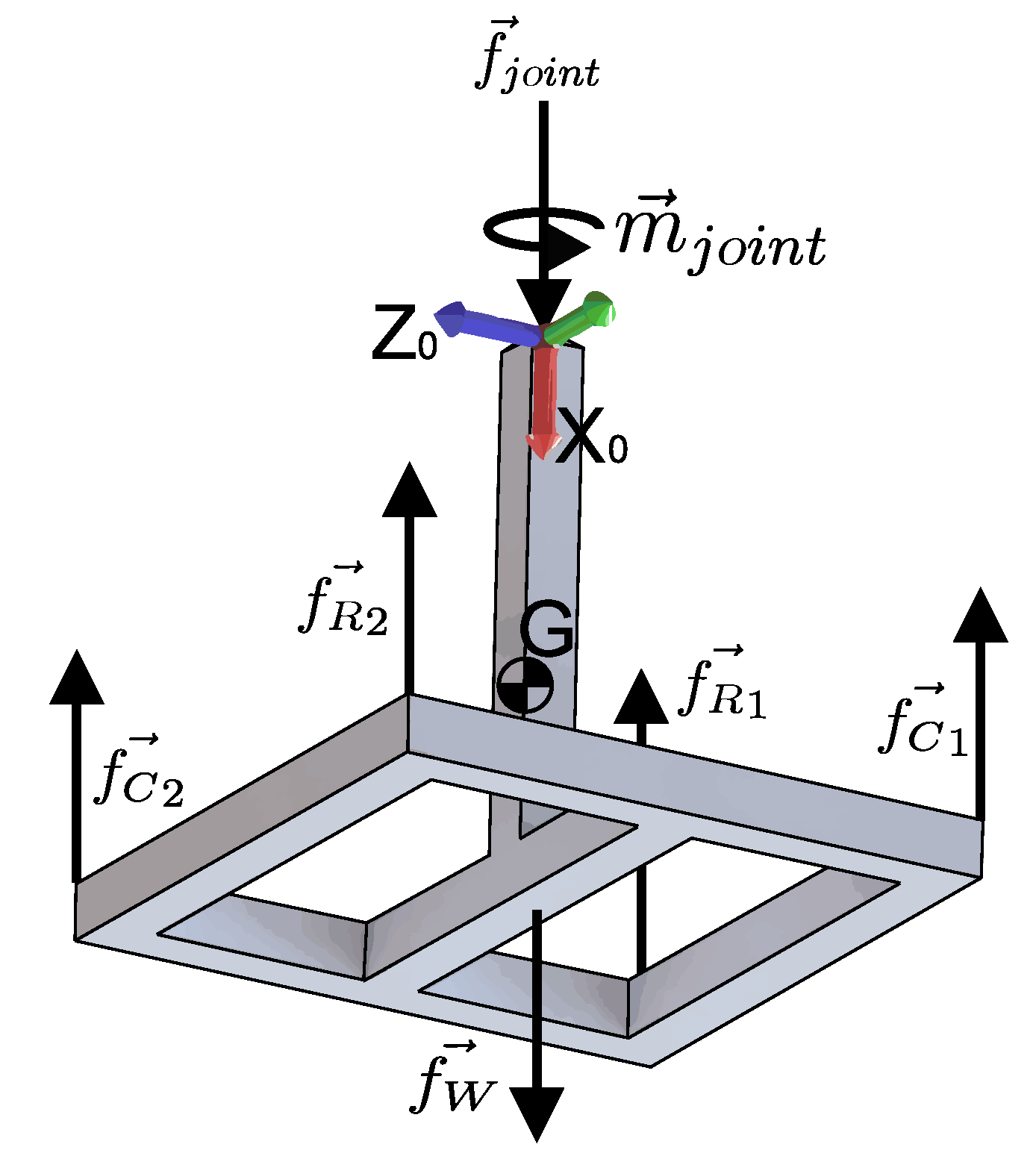
When replacing the fixed base, as well as the flexible elements by the forces and moments that the aforementioned elements exert on the moving platform, it results in the free-body diagram used for the static analysis shown in Figure 5.

Forces ${\overrightarrow{f}}_{{\mathrm{C}}_1}$ and ${\overrightarrow{f}}_{{\mathrm{C}}_2}$ refer to the forces exerted by cables ${\mathrm{C}}_1$ and ${\mathrm{C}}_2$, respectively, on the moving platform. Similarly, forces ${\overrightarrow{f}}_{R_1}$ and ${\overrightarrow{f}}_{R_2}$ denote the forces exerted by the springs ${\mathrm{r}}_1$ and ${\mathrm{r}}_2$, respectively. Force ${\overrightarrow{f}}_W$ represents the force exerted by the action of gravity on the moving platform applied to the centroid, G, of the robot. Finally, the force-torque system composed by the force ${\overrightarrow{f}}_{joint}$ and the moment ${\overrightarrow{m}}_{joint}$ represents the reaction force and moment exerted by the universal joint on the moving platform.

Applying the equilibrium conditions embodied in Equations (20) and (21):

$$\begin{array}{ccc}\hfill {\overrightarrow{f}}_{{\mathrm{C}}_1}+{\overrightarrow{f}}_{{\mathrm{C}}_2}+{\overrightarrow{f}}_{R_1}+{\overrightarrow{f}}_{R_2}+{\overrightarrow{f}}_W+{\overrightarrow{f}}_{joint}& =& \overrightarrow{0}\hfill \end{array}$$

(22)

$$\begin{array}{ccc}\hfill {\overrightarrow{r}}_{M_{1/0}}\times {\overrightarrow{f}}_{{\mathrm{C}}_1}+{\overrightarrow{r}}_{M_{2/0}}\times {\overrightarrow{f}}_{{\mathrm{C}}_2}+{\overrightarrow{r}}_{R_{1/0}}\times {\overrightarrow{f}}_{R_1}+{\overrightarrow{r}}_{R_{2/0}}\times {\overrightarrow{f}}_{R_2}+{\overrightarrow{r}}_{G/0}\times {\overrightarrow{f}}_W+{\overrightarrow{m}}_{joint}& =& \overrightarrow{0}\hfill \end{array}$$

(23)

From the solution of Equations (22) and (23), the magnitudes of the forces and moments $\left|{\overrightarrow{f}}_{{\mathrm{C}}_1}\right|$, $\left|{\overrightarrow{f}}_{{\mathrm{C}}_2}\right|$, $\left|{\overrightarrow{f}}_{R_1}\right|$, $\left|{\overrightarrow{f}}_{R_2}\right|$, $\left|{\overrightarrow{f}}_{joint}\right|$ and $\left|{\overrightarrow{m}}_{joint}\right|$ are obtained, which ensures that the tensegrity robot is in static equilibrium.

4. Form Finding Analysis

In this section, we present the proposed methodology for the form-finding analysis of the class 2 tensegrity robot, including a numerical example applying this methodology.

4.1. Methodology Proposed

The proposed methodology for the form-finding analysis of the class 2 tensegrity robot analyzed in this paper consists of finding all the possible geometric configurations of equilibrium that the robot can adopt. This is by performing the forward kinematic position analysis in combination with the static analysis for each of the geometrical configurations defined by the joint variables ${\theta }_1$ and ${\theta }_2$.

The geometric configurations analyzed were defined through the set of joint coordinates $\left\{{\theta }_{1{}_i},{\theta }_{2{}_i}\right\}$. For each ${\theta }_{1{}_i}$, there exists a set ${\Lambda }_i=\left\{{\theta }_{2{}_j}\right\}$ with $j=1,2,...,n$, and $i=1,2,...,n$. Thus,

$$\begin{array}{c}\hfill {\Lambda }_i=\left\{{\theta }_{2{}_1},{\theta }_{2{}_2},{\theta }_{2{}_3},...,{\theta }_{2{}_n}\right\}\end{array}$$

(24)

Then, it is possible to get a set $\Omega$ that satisfies Equations (22) and (23), i.e.,

$$\begin{array}{ccc}\hfill \Omega =\{{\theta }_{1{}_i},{\Lambda }_i:{\overrightarrow{f}}_{{\mathrm{C}}_1}+{\overrightarrow{f}}_{{\mathrm{C}}_2}+{\overrightarrow{f}}_{R_1}+{\overrightarrow{f}}_{R_2}+{\overrightarrow{f}}_W+{\overrightarrow{f}}_{joint}& =& \overrightarrow{0},\hfill \\ \hfill {\overrightarrow{r}}_{M_{1/0}}\times {\overrightarrow{f}}_{{\mathrm{C}}_1}+{\overrightarrow{r}}_{M_{2/0}}\times {\overrightarrow{f}}_{{\mathrm{C}}_2}+{\overrightarrow{r}}_{R_{1/0}}\times {\overrightarrow{f}}_{R_1}+{\overrightarrow{r}}_{R_{2/0}}\times {\overrightarrow{f}}_{R_2}+{\overrightarrow{r}}_{G/0}\times {\overrightarrow{f}}_W+{\overrightarrow{m}}_{joint}& =& \overrightarrow{0}\}\hfill \end{array}$$

(25)

By solving the system of equations obtained by the equilibrium conditions embodied in Equations (22) and (23) for each of the n geometrical configurations, the magnitudes of the forces and moments $\left|{\overrightarrow{f}}_{\mathrm{C}{}_{1_i}}\right|$, $\left|{\overrightarrow{f}}_{\mathrm{C}{}_{2_i}}\right|$, $\left|{\overrightarrow{f}}_{R{}_{1_i}}\right|$, $\left|{\overrightarrow{f}}_{R{}_{2_i}}\right|$, $\left|{\overrightarrow{f}}_{join{t}_i}\right|$, and $\left|{\overrightarrow{m}}_{join{t}_i}\right|$ corresponding to the ith geometric configuration analyzed are obtained.

Furthermore, to consider a particular geometrical configuration as geometric equilibrium configuration, it is necessary that the values of the forces and moments calculated comply with the condition

$$\begin{array}{c}\hfill \begin{array}{ccc}\left|{\overrightarrow{f}}_{\mathrm{C}{}_{1_i}}\right|\ge 0& ,& \left|{\overrightarrow{f}}_{\mathrm{C}{}_{2_i}}\right|\ge 0\\ \left|{\overrightarrow{f}}_{R{}_{1_i}}\right|\ge 0& ,& \left|{\overrightarrow{f}}_{R{}_{2_i}}\right|\ge 0\\ \left|{\overrightarrow{f}}_{join{t}_i}\right|\le 0& ,& \left|{\overrightarrow{m}}_{join{t}_i}\right|=0\end{array}\end{array}$$

(26)

By fulfilling the conditions of Equation (26), it is ensured that the class 2 tensegrity robot is in equilibrium and, moreover, it is ensured that the forces contained in its flexible elements are only tension forces while the forces contained in the rigid elements are exclusively compression forces.

Then, Equation (25) can be constrained using Equation (26) as follows:

$$\begin{array}{c}\hfill \Omega =\left\{{\theta }_{1{}_i},{\Lambda }_i:\left|{\overrightarrow{f}}_{\mathrm{C}{}_{1_i}}\right|\ge 0,\left|{\overrightarrow{f}}_{\mathrm{C}{}_{2_i}}\right|\ge 0,\left|{\overrightarrow{f}}_{R{}_{1_i}}\right|\ge 0,\left|{\overrightarrow{f}}_{R{}_{2_i}}\right|\ge 0,\left|{\overrightarrow{f}}_{join{t}_i}\right|\le 0,\left|{\overrightarrow{m}}_{join{t}_i}\right|=0\right\}\end{array}$$

(27)

4.2. Numerical Example

For the implementation of the methodology presented in the previous section, the geometric specifications listed in

Table 2. Form-finding parameters.

Definition	Variable	Value
Distance from the common point of the axes ${\theta }_1$ and ${\theta }_2$ to the moving platform	$a_2$	210 mm
Distance from the fixed base to the common point of the axes ${\theta }_1$ and ${\theta }_2$	${\mathit{l}}_1$	190 mm
Width of the moving platform	${\mathit{l}}_2$	220 mm
Initial condition of ${\theta }_1$	${\theta }_{1,1}$	−0.5236 rad
Initial condition of ${\theta }_2$	${\theta }_{2,1}$	−0.5236 rad
Joints coordinate increment	$\Delta \theta$	0.0087 rad
Number of geometrical configuration analyzed	n	14761
Initial x coordinate of the centroid, G, with respect to the reference frame ${\Sigma }_W$	$x_{ce}$	354.0442 mm
Initial y coordinate of the centroid, G, with respect to the reference frame ${\Sigma }_W$	$y_{ce}$	0 mm
Initial z coordinate of the centroid, G, with respect to the reference frame ${\Sigma }_W$	$z_{ce}$	76.4886 mm
Mass of the moving platform	m	0.4732 kg

are proposed.

By substituting the parameters listed in Table 2 in the forward kinematic of position (Equations (6)–(13)), the coordinates of M, $M_1$, $M_2$, ${\mathrm{r}}_1$, and ${\mathrm{r}}_2$ are obtained (see Figure 2), as well as the middle points of the superior base known by design $B_1$, $B_2$, $B_3$, $B_4$, ${\Sigma }_0$, and G. With the aforementioned information, the numerical evaluation of Equation (25) is computed, providing a matrix of points, as shown in blue in Figure 6, which represents the possible geometric configurations of the class 2 tensegrity robot. However, only the matrix of points represented in red in Figure 6 fulfill the equilibrium conditions represented by Equation (27), i.e., the workspace of the robot.

Figure 7 shows the geometric configurations analyzed, in the Y–Z plane. In this plane, the set of geometric equilibrium configurations (red points) within which the class 2 tensegrity robot can migrate from one geometric configuration to another without collapsing in the process can be seen.

5. Numerical Experiments

This section presents the numerical examples used to corroborate and compare the results obtained from the static analysis using Equations (22) and (23) and static analysis using ANSYS${}^{\copyright }$. Four different cases were reviewed, choosing values of the joint variables for positions within the workspace of the tensegrity robot.

The parameters remain the same from the previous section, and the selected values for the joint variables are shown in

Table 3. Selected positions for static analysis.

Experiment	${\mathit{\theta }}_1$ (rad)	${\mathit{\theta }}_2$ (rad)
1	0.0941	0.0332
2	0.0854	−0.0277
3	−0.0625	0.0245
4	−0.0799	−0.0364

.

The geometrical configurations adopted by the robot for these values of ${\theta }_1$ and ${\theta }_2$ were tested using Equations (22) and (23) and were found to be in static equilibrium satisfying Equation (27). Now, to corroborate these results, the software ANSYS${}^{\copyright }$ was used to perform a static analysis on a model of the moving platform oriented in the desired analysis position, adequately constrained, to check if this truly is a configuration capable of maintaining static equilibrium.

To create a reliable model of the tensegrity robot, BEAM188 elements were used to represent the rigid bars, since this type of elements is suitable for analyzing slender 3D beam structures. The element has two nodes and six degrees of freedom at each node.

For the two cables ${\mathrm{C}}_1$ and ${\mathrm{C}}_2$, LINK180 element was selected. LINK180 is a 3D spar used to model trusses, sagging cables, links, and springs, among others. The element is a uniaxial tension–compression element with three degrees of freedom at each node.

Finally, for the two springs ${\mathrm{r}}_1$ and ${\mathrm{r}}_2$, COMBIN14 elements were chosen, which is a uniaxial tension–compression element with up to three degrees of freedom at each node used to represent combined spring–damper elements. The type of elements used for the discretization of the moving platform of the class 2 tensegrity robot for the simulation in software ANSYS${}^{\copyright }$ is shown in

Table 4. Type of elements.

Element Number	Physical Element	Element Type
1	Rigid elements	BEAM188
2	Cable ${\mathrm{C}}_1$	LINK180
3	Cable ${\mathrm{C}}_2$	LINK180
4	Spring ${\mathrm{r}}_1$	COMBIN14
5	Spring ${\mathrm{r}}_2$	COMBIN14

.

Figure 8a shows the graphic form of the data mentioned in Table 4. Figure 8b shows the nodes of the discretized elements. Nodes 1–4 represent the union of the flexible elements with the moving platform, boundary conditions for which are constrained in translation and rotation in all directions. Node 8 represents the universal joint which boundary conditions are constrained in translation in all directions and the rotation around the X-axis. Node 9 represents the centroid of the moving platform, which is where an external force corresponding to gravity is applied. On the other hand, Nodes 10–16 have neither constraints nor applied forces.

Figure 9 shows graphically the geometric configurations listed in Table 3 for each of the numerical experiments.

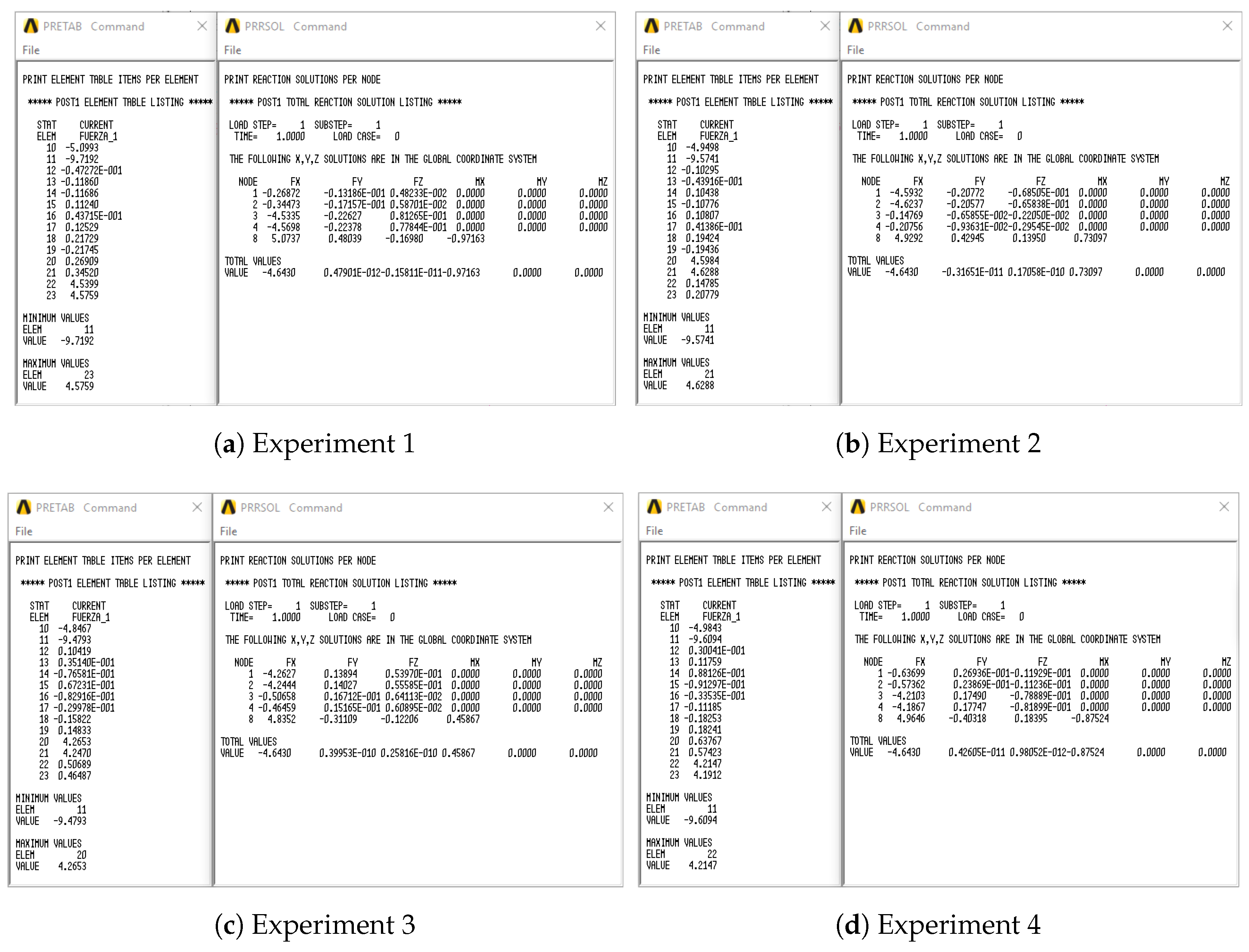
Figure 10 shows results from the software ANSYS${}^{\copyright }$ of the four numerical experiments. In addition, a comparative table between the values obtained from the proposed method and the software for each experiment is shown in

Table 5. Comparison between analytical and software results.

Experiment 1
	Analytical	ANSYS${}^{\copyright }$	Error
$\left|{\overrightarrow{f}}_{{\mathrm{C}}_1}\right|$	0.28507 N	0.26909 N	5.60%
$\left|{\overrightarrow{f}}_{{\mathrm{C}}_2}\right|$	0.36316 N	0.34520 N	4.94%
$\left|{\overrightarrow{f}}_{R_1}\right|$	4.5394 N	4.5399 N	0.01%
$\left|{\overrightarrow{f}}_{R_2}\right|$	4.5765 N	4.5759 N	0.01%
$\left|{\overrightarrow{f}}_{joint}\right|$	5.1333 N	5.0993 N	0.66%
$\left|{\overrightarrow{m}}_{joint}\right|$	0.97461 N·mm	0.97163 N·mm	0.30%
Experiment 2
	Analytical	ANSYS${}^{\copyright }$	Error
$\left|{\overrightarrow{f}}_{{\mathrm{C}}_1}\right|$	4.6879 N	4.5984 N	1.90%
$\left|{\overrightarrow{f}}_{{\mathrm{C}}_2}\right|$	4.7231 N	4.6288 N	1.99%
$\left|{\overrightarrow{f}}_{R_1}\right|$	0.14290 N	0.14785 N	3.46%
$\left|{\overrightarrow{f}}_{R_2}\right|$	0.21225 N	0.20779 N	2.10%
$\left|{\overrightarrow{f}}_{joint}\right|$	5.1331 N	4.9498 N	3.57%
$\left|{\overrightarrow{m}}_{joint}\right|$	$-0.74492$ N·mm	$-0.73097$ N·mm	1.87%
Experiment 3
	Analytical	ANSYS${}^{\copyright }$	Error
$\left|{\overrightarrow{f}}_{{\mathrm{C}}_1}\right|$	4.4108 N	4.2653 N	3.29%
$\left|{\overrightarrow{f}}_{{\mathrm{C}}_2}\right|$	4.3877 N	4.2470 N	3.20%
$\left|{\overrightarrow{f}}_{R_1}\right|$	0.51232 N	0.50689 N	1.05%
$\left|{\overrightarrow{f}}_{R_2}\right|$	0.45902 N	0.46487 N	1.27%
$\left|{\overrightarrow{f}}_{joint}\right|$	5.1324 N	4.8467 N	5.56%
$\left|{\overrightarrow{m}}_{joint}\right|$	$-0.47259$ N·mm	$-0.45867$ N·mm	2.94%
Experiment 4
	Analytical	ANSYS${}^{\copyright }$	Error
$\left|{\overrightarrow{f}}_{{\mathrm{C}}_1}\right|$	0.71580 N	0.63767 N	10.91%
$\left|{\overrightarrow{f}}_{{\mathrm{C}}_2}\right|$	0.64452 N	0.57423 N	10.90%
$\left|{\overrightarrow{f}}_{R_1}\right|$	4.2162 N	4.2147 N	0.03%
$\left|{\overrightarrow{f}}_{R_2}\right|$	4.1898 N	4.1912 N	0.03%
$\left|{\overrightarrow{f}}_{joint}\right|$	5.1328 N	4.9843 N	2.89%
$\left|{\overrightarrow{m}}_{joint}\right|$	0.88771 N·mm	0.87524 N·mm	1.40%

. Notice that, in ANSYS${}^{\copyright }$, Elements 20–23 represent cable ${\mathrm{C}}_1$, cable ${\mathrm{C}}_2$, spring ${\mathrm{r}}_1$ and spring ${\mathrm{r}}_2$, respectively. In addition, Node 8 is the point where the universal joint is located, meaning that force and moment reactions in this node are the reactions of the joint. The results in Table 5 show that the error percentage increases as the geometric configurations of equilibrium of the class 2 tensegrity robot approaches the blue points matrix shown in Figure 6 and Figure 7.

The results of the proposed methodology are proven with the results of the numerical experiments. In addition, these results guarantee that the class 2 tensegrity robot is in equilibrium for the geometric configuration analyzed.

6. Conclusions

This paper presents the form-finding analysis methodology for a class 2 tensegrity robot, which is classified in part of the literature as a soft robot because its structure presents a combination of rigid elements and mostly flexible elements. Two-thirds of the class 2 tensegrity robots analyzed as a case of study in the present work are flexible elements.

The form-finding analysis methodology employs basic tools of linear algebra instead of the strategies used in the literature, which uses genetic algorithms and neural networks, among others. The methodology consists of two steps: kinematic analysis and static analysis. The analysis of the possible geometric configurations of the robot is carried out through the results of the kinematic position analysis; nevertheless, it must guarantee which of those geometric configurations so that the robot does not collapse. From the static analysis, the equilibrium positions of the robot are found, which represents the workspace within which the class 2 tensegrity robot can migrate from one geometric configuration to another without collapsing in the process.

Four points of the workspace were selected to perform numerical experiments using the finite element analysis software ANSYS${}^{\copyright }$, which proved the results of the proposed methodology. It also verified that the robot is in equilibrium with the geometric configuration analyzed. The results shown in Table 5 give a reference to develop a prototype for the class 2 tensegrity robot.