Heuristic Approaches to Attribute Reduction for Generalized Decision Preservation

Abstract

Attribute reduction is a challenging problem in rough set theory, which has been applied in many research fields, including knowledge representation, machine learning, and artificial intelligence. The main objective of attribute reduction is to obtain a minimal attribute subset that can retain the same classification or discernibility properties as the original information system. Recently, many attribute reduction algorithms, such as positive region preservation, generalized decision preservation, and distribution preservation, have been proposed. The existing attribute reduction algorithms for generalized decision preservation are mainly based on the discernibility matrix and are, thus, computationally very expensive and hard to use in large-scale and high-dimensional data sets. To overcome this problem, we introduce the similarity degree for generalized decision preservation. On this basis, the inner and outer significance measures are proposed. By using heuristic strategies, we develop two quick reduction algorithms for generalized decision preservation. Finally, theoretical and experimental results show that the proposed heuristic reduction algorithms are effective and efficient.

1. Introduction

Originating from the mathematician Pawlak in the early 1980s, rough set theory (RST) [1] has been regarded as an effective tool for the processing of inconsistent or uncertain information. It has been extensively utilized in research fields such as uncertainty reasoning [2,3], knowledge representation [4], feature selection, and machine learning [5,6,7]. Attribute reduction [1,8,9,10] plays a crucial role in RST. The main purpose of attribute reduction is to find a minimal attribute subset which has the same classification or discernibility properties as the original information system. Different attribute reductions can leave different classification or discernibility properties of information systems unchanged. For example, positive region preservation reduction [11] can leave the positive region of a target decision unchanged. Generalized decision preservation reduction [12,13] can leave the generalized decision of each object in the universe unchanged. Mutual information preservation reduction [14] can leave mutual information, with respect to the decision attributes, unchanged. In the last twenty years, many methods for attribute reduction have been studied, such as discernibility matrix-based attribute reduction methods [15,16,17,18,19,20], heuristic attribute reduction methods [10,21,22,23], metaheuristic attribute reduction methods [24,25,26,27,28,29,30], and so on.

In attribute reduction, the discernibility matrix is an important technique for obtaining all reducts from data sets. Skowron et al. [8] first proposed a discernibility matrix which can obtain all reducts from an information system. To extend the classical discernibility matrix, many methods of discernibility matrix-based attribute reduction have been studied. Based on the similarity relation, Kryszkiewicz [13] proposed discernibility matrices in incomplete information systems. By using maximal consistent blocks in incomplete information systems, Leung et al. [31] proposed a more efficient computational method for attribute reduction. Miao et al. [32] introduced an attribute reduction method which can leave maximal consistent blocks unchanged in an interval-valued information system. To obtain the reducts, with respect to one decision class instead of all decision classes, Liu et al. [33] constructed discernibility matrices regarding lth lower approximation reduction, lth decision class reduction, and $\beta$-reduction of the lth decision class. Miao et al. [12] proposed a theoretical framework for discernibility matrix-based attribute reduction. Based on this framework, the generalized discernibility matrix was constructed.

As mentioned above, all reducts can be found by using discernibility matrices. However, finding all reducts from a decision system based on a discernibility matrix has been proved to be an NP-hard problem. Therefore, the aforementioned methods based on discernibility matrices are inefficient and difficult to apply in large-scale data sets. To increase the efficiency of attribute reduction, many methods of heuristic attribute reduction and metaheuristic attribute reduction have been researched extensively. Hu et al. [11] first introduced a heuristic method for positive region reduction. Using the mutual information, Miao et al. [14] proposed a bottom-up reduction algorithm. Qian et al. [34] closely focused on increasing the efficiencies of heuristic reduction algorithms, and adopted a positive approximation strategy to accelerate heuristic reduction algorithms. Dai et al. [35] used a variant form of conditional entropy to design an attribute reduction algorithm for an interval-valued decision system. Many attribute reduction algorithms based on metaheuristic methods [24,25,26,27,28,29,30,36,37] have been developed recently. Chebrolu et al. [26] used a genetic algorithm to obtain a global minimal reduct in a decision-theoretic rough set model. By using ant colony optimization, Chen et al. [29] gave a feature selection algorithm which can find minimal subset of the features. Min et al. [30] investigated a partial-complete searching method for ant colony optimization and developed an algorithm for time-cost sensitive attribute reduction. Jia et al. [36] researched minimum cost attribute reduction by using simulated annealing and genetic algorithms. Metaheuristic attribute reduction is an active and important research field in attribute reduction. Compared with heuristic attribute reduction methods, some significant research results by using metaheuristic attribute reduction methods have been achieved. Chebrolu et al. [25] developed a metaheuristic attribute reduction algorithm for real-valued data, called the hybrid ABC-EFTSBPSD. Comparative experiments were conducted to verify the performance of the hybrid ABC-EFTSBPSD and the following two conclusions were obtained: (1) The length of a reduct calculated by the hybrid ABC-EFTSBPSD was shorter than those of reducts calculated by the heuristic reduction algorithms (ACO-RST [27], Q-MDRA [38], and IMCVR [39]), in most cases. (2) By employing C4.5 and SVM classifiers, the hybrid ABC-EFTSBPSD had higher classification accuracies than the heuristic reduction algorithms (Q-MDRA, ACO-RST, and IMCVR). Compared with the heuristic attribute reduction methods MIBR [14] and QUICKREDUCT [24], the algorithm RSFSACO, based on ant colony optimization, proposed by Chen et al. [29] could obtain a minimal reduct in most cases.

In a decision system, objects with the same condition attribute values may have different decision values. To keep these decision values unchanged, Miao et al. [12] proposed an attribute reduction method for generalized decision preservation based on the discernibility matrix. Based on this method, one can find all reducts for generalized decision preservation from a decision system. In constructing a discernibility matrix and translating a conjunctive normal form (CNF) into a disjunctive normal form (DNF) in a discernibility function, discernibility matrix-based reduction algorithms for generalized decision preservation are computationally time-consuming and impractical when dealing with large amounts of data. To address this problem, we introduce the similarity degree for generalized decision preservation. By using the inner and outer significance measures, we develop two quick reduction algorithms for generalized decision preservation. Theoretical analyses and experimental results show that two proposed algorithms are feasible and efficient.

The novelties and contributions of this paper can be summarized as follows: First, a similarity measure for generalized decision preservation has not yet been proposed so far. Hence, in order to measure the similarity of attributes for generalized decision preservation, we introduce a novel monotonic similarity degree in this paper. Second, to evaluate the significance of an attribute for generalized decision preservation, we propose two significance measures (the inner and outer significance measures for generalized decision preservation), based on the proposed similarity degree. Third, we use the add-deleting and deleting strategies to design forward and backward greedy reduction algorithms for generalized decision preservation (FGRAG and BGRAG). If m denotes the number of condition attributes and n indicates the number of objects, the time complexities of FGRAG and BGRAG are $O\left(m^{3}n\right)$ and $O\left(m^{2}n\right)$, respectively. The time complexity of the discernibility matrix-based reduction algorithm for generalized decision preservation (DMRAG) proposed by Miao et al. [12] is $O(m^{C_m^{⌈m/2⌉}}+m{n}^4)$. The running time of DMRAG increases distinctively when the number of attributes and objects increase. Meanwhile, the running time of FGRAG (BGRAG) is less than that of DMRAG, relatively. Thus, the proposed reduction algorithms (FGRAG and BGRAG) are more efficient. Experimental results indicate the subset calculated by FGRAG (BGRAG) is a reduct for generalized decision preservation in a decision system. Compared with DMRAG, FGRAG and BGRAG are more efficient when dealing with the same amount of attributes or objects. By avoiding calculating the core, BGRAG is usually more efficient than FGRAG, in many cases. Our work in this paper indicates how to simplify a decision system more quickly. Meanwhile, the generalized decision of each object in the universe is unchanged. These research results will be useful for multi-attribute decision analyses in practical applications.

The structure of this study is presented as follows: Some basic notions related to rough approximations and generalized decision preservation will be reviewed in the following section. In Section 3, the inner and outer significance measures are introduced to develop heuristic attribute reduction algorithms for generalized decision preservation. Then, forward and backward heuristic reduction algorithms are proposed. Comparative experiments are conducted to verify monotonicity of the similarity degree, correctness, and efficiency of the proposed heuristic reduction algorithms in Section 4. Finally, the entire work is summarized in Section 5.

2. Preliminaries

2.1. Rough Approximations in a Decision System

In this section, we will review some fundamental notions of RST [1], such as a decision system, discernibility relation, and rough approximation. Studies of RST typically start with the concept of a decision system. Assume that $U=\{x_1,x_2,\dots ,x_n\}$ is the universe, $C=\{a_1,a_2,...,a_m\}$ and $D=\left\{d\right\}$ are a condition attribute set and a decision attribute set, $V_a$ is the domain of attribute values for all $a\in AT$, and $I_a:U\times \left\{a\right\}\to V_a$ is an information function such that $I(x,a)=a\left(x\right)\in V_a$ for all $x\in U$ and $a\in AT$. Then, the 4-tuple $DS=(U,C\cup D,V_a,I_a)$ is referred as to a decision system [1] in RST. For brevity, a decision system can be also denoted by a 2-tuple $DS=(U,C\cup D)$. For instance,

Table 1. A decision system.

U	${\mathit{a}}_1$	${\mathit{a}}_2$	${\mathit{a}}_3$	${\mathit{a}}_4$	d
$x_1$	1	1	2	4	2
$x_2$	1	1	2	4	1
$x_3$	1	1	2	4	1
$x_4$	1	1	3	4	1
$x_5$	1	1	3	4	3
$x_6$	2	2	3	4	2
$x_7$	2	2	3	4	1
$x_8$	2	2	3	4	2

shows a decision system $DS=(U,C\cup D,V_a,I_a)$, where the universe is $U=\{x_1,x_2,x_3,x_4,x_5,x_6,x_7,x_8\}$, the condition attribute set is $C=\{a_1,a_2,a_3,a_4\}$, and the decision attribute set is $D=\left\{d\right\}$.

Definition 1.

[1] Given a decision system $DS=(U,C\cup D,V_a,I_a)$, for $\forall Q\subseteq C$, if $x_i,x_j\in U$, $a\left(x_i\right)$ and $a\left(x_j\right)$ are the values of objects $x_i$ and $x_j$, with respect to the attribute a, and the indiscernibility relation regarding Q is defined as

$$Ind\left(Q\right)=\{(x_i,x_j)\in U\times U|\forall a\in Q,a\left(x_i\right)=a\left(x_j\right)\}.$$

(1)

Obviously, $Ind\left(Q\right)$ is symmetric, transitive, and reflexive. Hence, $Ind\left(Q\right)$ is an equivalence relation and can be calculated as $Ind\left(Q\right)={\bigcap }_{a\in Q}Ind\left(\left\{a\right\}\right)$. $Ind\left(Q\right)$ divides the universe U into a collection of indiscernible granules (equivalence classes); that is, $U/Ind\left(Q\right)=U/Q=\left\{E_{IND\left(Q\right)}\left(x_i\right)\right|x_i\in U\}=\left\{E_Q\left(x_i\right)\right|x_i\in U\}$, where $E_{IND\left(Q\right)}\left(x_i\right)=E_Q\left(x_i\right)$ is an indiscernible granule containing $x_i$. From classical RST, indiscernible granules can constitute two definable sets, called the lower approximation and the upper approximation. An arbitrary decision class in the universe can be approximated by the lower and upper approximations, which are defined as follows:

Definition 2.

[1] Given a decision system $DS=(U,C\cup D,V_a,I_a)$, $\forall Q\subseteq C$, $D_j\in U/D$, the lower approximation (LA) and the upper approximation (UA) of $D_j$, with respect to Q, are defined as follows:

$${\underline{Apr}}_Q\left(D_j\right)=\left\{x_i\right|E_Q\left(x_i\right)\subseteq D_j\}=\bigcup \left\{E_Q\left(x_i\right)\right|E_Q\left(x_i\right)\subseteq D_j\},$$

(2)

$${\overline{Apr}}_Q\left(D_j\right)=\left\{x_i\right|E_Q\left(x_i\right)\cap D_j\ne \varnothing \}=\bigcup \left\{E_Q\left(x_i\right)\right|E_Q\left(x_i\right)\cap D_j\ne \varnothing \}.$$

(3)

For $\forall Q\subseteq C$, ${\underline{Apr}}_Q\left(D_j\right)$ is the union of all $E_Q\left(x_i\right)$ which are included in $D_j$ totally, whereas ${\overline{Apr}}_Q\left(D_j\right)$ is the union of all $E_Q\left(x_i\right)$ which are included in $D_j$ partially. $U-{\overline{Apr}}_Q\left(D_j\right)$ is the union of the $E_Q\left(x_i\right)$ which are not included in $D_j$ completely. The positive region (PR), boundary region (BR), and negative region (NR) of $D_j$ in the universe are defined, respectively, as follows: $Po{s}_Q\left(D_j\right)={\underline{Apr}}_Q\left(D_j\right)$, $Bn{d}_Q\left(D_j\right)={\overline{Apr}}_Q\left(D_j\right)-{\underline{Apr}}_Q\left(D_j\right)$, and $Ne{g}_Q\left(D_j\right)=U-{\overline{Apr}}_Q\left(D_j\right)$.

The relationship among the three regions (PR, BR, and NR) is presented as follows:

$$Po{s}_Q\left(D_j\right)+Bn{d}_Q\left(D_j\right)+Ne{g}_Q\left(D_j\right)=U.$$

(4)

Definition 3.

[1] For a decision system $DS=(U,C\cup D,V_a,I_a)$, $DS$ is consistent if and only if ${\bigcup }_{j=1}^{|U/D|}Po{s}_C\left(D_j\right)=U$; otherwise, $DS$ is inconsistent.

In an inconsistent decision system $DS=(U,C\cup D,V_a,I_a)$, there must exist $x_i,x_j\in U(i\ne j)$ such that $(x_i,x_j)\in Ind\left(Q\right)$ but $d\left(x_i\right)\ne d\left(x_j\right)$. Rough approximations are closely related to decision rules in a decision system. The decision rule regarding an object in the positive region is a certainty rule in a decision system; otherwise, the decision rule is an uncertainty rule.

2.2. Discernibility Matrix-Based Attribute Reduction for Generalized Decision Preservation

In this section, we review the concept of generalized decision and attribute reduction for generalized decision preservation based on the discernibility matrix. In inconsistent information systems, objects with the same condition attribute values may have different decision values. The set of these decision values is called the generalized decision [12], which is defined as follows:

Definition 4.

[12] Given a decision system $DS=(U,C\cup D,V_a,I_a)$, for all $x_i,x_j\in U$, $\forall Q\subseteq C$, $E_Q\left(x_i\right)\in U/Q$, the generalized decision for an object $x_i$, with respect to Q, is defined as

$${\delta }_Q\left(x_i\right)=\left\{f(x_j,d)\right|x_j\in E_Q\left(x_i\right)\}.$$

(5)

For all $x_i\in U$, it is easy to observe that $1\le |{\delta }_Q\left(x_i\right)|\le |U|$. For all $x_i\in U$, if $|{\delta }_Q\left(x_i\right)|=1$, then an arbitrary object in a decision system has a unique decision value. Then, $DS$ is a consistent decision system (or, we say that $DS$ is consistent); otherwise, $DS$ is inconsistent. In an inconsistent decision system, there exists at least one object with multiple decision values.

A reduct can provide a minimal attribute subset which contains the same classification properties as the original condition attribute set. Attribute reduction for generalized decision preservation can keep the possible decision values of each object unchanged. Therefore, a reduct for generalized decision preservation [12] can be defined as follows:

Definition 5.

[12] Given a decision system $DS=(U,C\cup D,V_a,I_a)$, for all $x_i\in U$, $\exists x_j\in U$, $Q\subseteq C$ is a reduct for generalized decision preservation in $DS$ if and only if

(1) 

${\delta }_Q\left(x_i\right)={\delta }_C\left(x_i\right)$;

(2) 

$\forall P\subset Q,{\delta }_P\left(x_j\right)\ne {\delta }_Q\left(x_j\right)$.

To get all reducts of a decision system for generalized decision preservation, Miao et al. [12] described the discernibility matrix and its function for generalized decision preservation, as follows:

Definition 6.

[12] Given a decision system $DS=(U,C\cup D,V_a,I_a)$, for all $x_i,x_j\in U$, $a\in C$, the discernibility matrix for generalized decision preservation is given by

$$M_{decision}(x_i,x_j)=\left\{\begin{array}{cc}\left\{a\right|f(x_i,a)\ne f(x_j,a)\},\hfill & {\delta }_C\left(x_i\right)\ne {\delta }_C\left(x_j\right).\hfill \\ \varnothing ,\hfill & otherwise.\hfill \end{array}\right.$$

(6)

Definition 7.

[12] Given a decision system $DS=(U,C\cup D,V_a,I_a)$, if $M_{decision}(x_i,x_j)\ne \varnothing$, then the discernibility function of $DS$ can be denoted by

$$D{F}_{decision}(a_1,a_2,\dots ,a_{\left|C\right|})=\wedge \{\vee \left(M_{decision}(x_i,x_j)\right)|1\le i\le j\le |U\left|\right\}.$$

(7)

A discernibility matrix provides a matrix description of discernible attributes. Regarding discernible attributes as literals in a clause, we construct a discernibility function, which is a conjunctive normal form. We translate a conjunctive normal form (CNF) into a disjunctive normal form (DNF) by using Boolean operation laws. For a DNF, the set of literals in a clause is a reduct in a decision system. Based on the discernibility matrix and its function for generalized decision preservation, Miao et al. [12] introduced a discernibility matrix-based attribute reduction method for generalized decision preservation in Algorithm 1.

Algorithm 1 A discernibility matrix-based reduction algorithm for generalized decision preservation (DMRAG)

Input: A decision system $DS=(U,C\cup D,V_a,I_a)$ Output: All reducts for generalized decision preservation of $DS$ 1: Calculate the generalized decision for each object and construct a discernibility matrix $M_{decision}$. 2: Calculate a discernibility function $D{F}_{decision}$ corresponding to $M_{decision}$. 3: Simplify the discernibility function $D{F}_{decision}$ by absorption law. 4: Transform $D{F}_{decision}$ into a disjunctive normal form by Boolean operation laws. 5: Simplify the discernibility function $D{F}_{decision}$ by absorption law. 6: Output all generalized decision preservation reducts of $DS$.

Suppose that m denotes the number of condition attributes and n indicates the number of objects. Then, the time complexity of constructing a discernibility matrix is $O\left(m{n}^2\right)$. The time complexities of simplifying a discernibility function and converting a discernibility function into a disjunctive normal form are $O\left(m{n}^4\right)$ and $m^{C_m^{⌈m/2⌉}}$. Thus, the time complexity of Algorithm 1 is $O(m^{C_m^{⌈m/2⌉}}+m{n}^4)$.

According to Algorithm 1, we can construct a discernibility function of the decision system shown in Table 1 as $D{F}_{decision}(a_1,a_2,a_3,a_4)=\left(a_3\right)\wedge (a_1\vee a_2)=(a_1\wedge a_3)\vee (a_2\wedge a_3)$. Hence, the reducts of $DS$ are $\{a_1,a_3\}$ and $\{a_2,a_3\}$.

3. Heuristic Attribute Reduction for Generalized Decision Preservation

In what follows, we start by detailing a monotonic similarity measure between different condition attributes for generalized decision preservation in Section 3.1. Then, we propose the inner and outer attribute significance measures and heuristic attribute reduction algorithms for generalized decision preservation (FGRAG and BGARG) in Section 3.2.

3.1. The Similarity Degree for Generalized Decision Preservation

In studies of heuristic attribute reduction, the attribute similarity measure (heuristic information, dependency degree) is an important factor. Recently, to obtain the various reducts, different similarity measures have been proposed in rough set theory, such as the positive dependency degree [1], information entropy [35], conditional entropy [40], and maximum decision entropy [41]. However, there have been few studies on the similarity measure for generalized decision preservation. Thus, to evaluate the similarity of different attributes for generalized decision preservation, we define the similarity degree for generalized decision preservation as follows:

Definition 8.

Given a decision system $DS=(U,C\cup D,V_a,I_a)$, $\forall Q\subseteq C$, if $E_Q\left(x_i\right)\in U/Q$, $E_C\left(x_i\right)\in U/C$, the similarity degree for generalized decision preservation is defined as

$$Sim(Q,C)=\left\{\begin{array}{cc}\frac{|{\bigcup }_{i=1}^{\left|U\right|}(E_Q\left(x_i\right)\cap E_C\left(x_i\right))|}{\left|U\right|},\hfill & {\delta }_Q\left(x_i\right)={\delta }_C\left(x_i\right).\hfill \\ 0,\hfill & otherwise.\hfill \end{array}\right.$$

(8)

To express the monotonic theorem of the similarity degree for generalized decision preservation, we need the following theorem.

Theorem 1.

Given a decision system $DS=(U,C\cup D,V_a,I_a)$, if, for all $x_i\in U$, $P\subseteq Q\subseteq C$, $E_P\left(x_i\right)$, $E_Q\left(x_i\right)$, and $E_C\left(x_i\right)$ are the equivalence classes that contain the object $x_i$ with respect to P, Q, and C, then we have

$${\delta }_C\left(x_i\right)\subseteq {\delta }_Q\left(x_i\right)\subseteq {\delta }_P\left(x_i\right).$$

(9)

Proof. 

From the basic properties of rough set theory, for $x_i\in U$, $\forall Q\subseteq C$, it is easy to get $E_C\left(x_i\right)\subseteq E_Q\left(x_i\right)$. Suppose that ${\delta }_C\left(x_i\right)\supset {\delta }_Q\left(x_i\right)$. Then, there exists $x_j\in U$ such that $d\left(x_j\right)\in {\delta }_C\left(x_i\right)$ but $d\left(x_j\right)\notin {\delta }_Q\left(x_i\right)$. Then, $x_j\in E_C\left(x_i\right)$ but $x_j\notin E_Q\left(x_i\right)$. Therefore, we have $E_C\left(x_i\right)\neg \subseteq E_Q\left(x_i\right)$. This is contrary to $E_C\left(x_i\right)\subseteq E_Q\left(x_i\right)$. Then, ${\delta }_C\left(x_i\right)\subseteq {\delta }_Q\left(x_i\right)$. Similarly, we have ${\delta }_Q\left(x_i\right)\subseteq {\delta }_P\left(x_i\right)$. From the discussion above, ${\delta }_C\left(x_i\right)\subseteq {\delta }_Q\left(x_i\right)\subseteq {\delta }_P\left(x_i\right)$ holds. This completes the proof. □

Definition 8 provides a similarity measure between different condition attribute sets for generalized decision preservation. For all $Q\subseteq C$, we have $0\le Sim(Q,C)\le 1$. The monotonicity of the similarity degree for generalized decision preservation is presented as follows:

Theorem 2.

Given a decision system $DS=(U,C\cup D,V_a,I_a)$, $\forall P\subseteq Q\subseteq C$, we have

$$Sim(P,C)\le Sim(Q,C).$$

(10)

Proof. 

For all $P\subseteq Q\subseteq C$, $x_i\in U$, if $E_P\left(x_i\right)\in U/P$, $E_Q\left(x_i\right)\in U/Q$ and $E_C\left(x_i\right)\in U/C$, then $E_C\left(x_i\right)\subseteq E_Q\left(x_i\right)\subseteq E_P\left(x_i\right)$. If $x_{im}\in E_P\left(x_i\right)$, then we have $E_P\left(x_i\right)=E_Q\left(x_{i1}\right)\cup E_Q\left(x_{i2}\right)\cup ...\cup E_Q\left(x_{it}\right)={\bigcup }_{m=1}^t{E}_Q\left(x_{im}\right)$, where $1\le t\le |E_P\left(x_i\right)|$. If ${\delta }_P\left(x_i\right)\ne {\delta }_C\left(x_i\right)$, then $E_P\left(x_i\right)\cap E_C\left(x_i\right)=0$. For $x_{im}\in E_P\left(x_i\right)$, if ${\delta }_Q\left(x_{im}\right)\ne {\delta }_C\left(x_{im}\right)$, then $E_Q\left(x_{im}\right)\cap E_C\left(x_{im}\right)=0$.

Suppose that $(E_P\left(x_i\right)\cap E_C\left(x_i\right))\supset {\bigcup }_{m=1}^t(E_Q\left(x_{im}\right)\cap E_C\left(x_{im}\right))$. There must exist $x_{is}$ such that $x_{is}\in (E_P\left(x_i\right)\cap E_C\left(x_i\right))$ but $x_{is}\notin {\bigcup }_{m=1}^t(E_Q\left(x_{im}\right)\cap E_C\left(x_{im}\right))$. Then, ${\delta }_P\left(x_{is}\right)={\delta }_C\left(x_{is}\right)$, but ${\delta }_Q\left(x_{is}\right)\ne {\delta }_C\left(x_{is}\right)$. From Theorem 1, for all $x_{is}\in U$, we have ${\delta }_C\left(x_{is}\right)\subseteq {\delta }_Q\left(x_{is}\right)\subseteq {\delta }_P\left(x_{is}\right)$. As ${\delta }_P\left(x_{is}\right)={\delta }_C\left(x_{is}\right)$, then ${\delta }_Q\left(x_{is}\right)={\delta }_C\left(x_{is}\right)$. This is contrary to ${\delta }_Q\left(x_{is}\right)\ne {\delta }_C\left(x_{is}\right)$. Thus, $(E_P\left(x_i\right)\cap E_C\left(x_i\right))\subseteq {\bigcup }_{m=1}^t(E_Q\left(x_{im}\right)\cap E_C\left(x_i\right))$ holds. It is obvious that $|(E_P\left(x_i\right)\cap E_C\left(x_i\right))|\le |{\bigcup }_{m=1}^t(E_Q\left(x_{im}\right)\cap E_C\left(x_{im}\right))|$. Hence, $|{\bigcup }_{i=1}^{\left|U\right|}(E_P\left(x_i\right)\cap E_C\left(x_i\right))|\le |{\bigcup }_{i=1}^{\left|U\right|}{\bigcup }_{m=1}^t(E_Q\left(x_{im}\right)\cap E_C\left(x_{im}\right))|$; namely, $|{\bigcup }_{i=1}^{\left|U\right|}(E_P\left(x_i\right)\cap E_C\left(x_i\right))|\le |{\bigcup }_{i=1}^{\left|U\right|}(E_Q\left(x_i\right)\cap E_C\left(x_i\right))|$. Thus, we have $\frac{|{\bigcup }_{i=1}^{\left|U\right|}(E_P\left(x_i\right)\cap E_C\left(x_i\right))|}{\left|U\right|}\le \frac{|{\bigcup }_{i=1}^{\left|U\right|}(E_Q\left(x_i\right)\cap E_C\left(x_i\right))|}{\left|U\right|}$. Therefore, for all $P\subseteq Q\subseteq C$, $Sim(P,C)\le Sim(Q,C)$. This completes the proof. □

An example is given to explain Theorem 2, as follows:

Example 1.

Consider the decision system shown in Table 1, $P=\{a_1,a_2\}$, we have

$E_P\left(x_1\right)=E_P\left(x_2\right)=E_P\left(x_3\right)=E_P\left(x_4\right)=E_P\left(x_5\right)=\{x_1,x_2,x_3,x_4,x_5\}$,

$E_P\left(x_6\right)=E_P\left(x_7\right)=E_P\left(x_8\right)=\{x_6,x_7,x_8\}$.

As $U/D=\{\{x_1,x_6,x_8\},\{x_2,x_3,x_4,x_7\},\left\{x_5\right\}\}$,

${\delta }_P\left(x_1\right)={\delta }_P\left(x_2\right)={\delta }_P\left(x_3\right)={\delta }_P\left(x_4\right)={\delta }_P\left(x_5\right)=\{1,2,3\}$,

${\delta }_P\left(x_6\right)={\delta }_P\left(x_7\right)={\delta }_P\left(x_8\right)=\{1,2\}$

For $C=\{a_1,a_2,a_3,a_4\}$, we have

$E_C\left(x_1\right)=E_C\left(x_2\right)=E_C\left(x_3\right)=\{x_1,x_2,x_3\}$, $E_C\left(x_4\right)=E_C\left(x_5\right)=\{x_4,x_5\}$,

$E_C\left(x_6\right)=E_C\left(x_7\right)=E_C\left(x_8\right)=\{x_6,x_7,x_8\}$.

As $U/D=\{\{x_1,x_6,x_8\},\{x_2,x_3,x_4,x_7\},\left\{x_5\right\}\}$, we have

${\delta }_C\left(x_1\right)={\delta }_C\left(x_2\right)={\delta }_C\left(x_3\right)={\delta }_C\left(x_6\right)={\delta }_C\left(x_7\right)={\delta }_C\left(x_8\right)=\{1,2\}$,

${\delta }_C\left(x_4\right)={\delta }_C\left(x_5\right)=\{1,3\}$.

Therefore, the similarity degree between the attribute sets P and C is calculated as follows,

$Sim(P,C)=\frac{|(E_P\left(x_6\right)\cap E_C\left(x_6\right))\cup (E_P\left(x_7\right)\cap E_C\left(x_7\right))\cup (E_P\left(x_8\right)\cap E_C\left(x_8\right))|}{\left|U\right|}=\frac{\left|\right\{x_6,x_7,x_8\left\}\right|}{8}=\frac{3}{8}$.

Analogously, the similarity degree between the attribute sets Q and C is calculated as follows,

$Sim(Q,C)=\frac{\left|\right(E_Q\left(x_1\right)\cap E_C\left(x_1\right)\cup (E_Q\left(x_2\right)\cap E_C\left(x_2\right))\cup ...\cup (E_Q\left(x_8\right)\cap E_C\left(x_8\right))|}{\left|U\right|}=\frac{|\{x_1,x_2,x_3\}\cup \{x_4,x_5\}\cup \{x_6,x_7,x_8\}|}{8}=1$.

From the discussion above, for $P\subset Q\subset C$, it follows that $0<SIM(P,C)<SIM(Q,C)=1$.

Based on the similarity degree for generalized decision preservation, Definition 5 can be written, equivalently, as follows:

Definition 9.

Given a decision system $DS=(U,C\cup D,V_a,I_a)$, $Q\subseteq C$ is a reduct for generalized decision preservation in $DS$ if and only if

(1) 

$Sim(Q,C)=1$;

(2) 

$\forall P\subset Q$, $Sim(P,Q)\ne 1$.

The first condition means that the attribute subset Q has the same similarity degree as the original attribute set C, and the second condition means that there is no dispensable or redundant attribute in Q. It should be considered that dispensable or indispensable attributes are suited to the classification properties in a decision system. For example, a dispensable attribute for positive preservation may be indispensable for conditional entropy preservation.

Considering monotonicity of the similarity degree for generalized decision preservation, we also have the following definition:

Definition 10.

Given a decision system $DS=(U,C\cup D,V_a,I_a)$, $Q\subseteq C$ is a reduct for generalized decision preservation in $DS$ if and only if

(1) 

$Sim(Q,C)=1$;

(2) 

$\forall P\subset Q$, $Sim(P,C)<SIM(Q,C)$.

For all $Q\subseteq C$, if $\exists a\in Q$ such that $Sim(Q,C)=Sim(Q-\{a\},C)$, then a is called a dispensable attribute for generalized decision preservation with respect to Q; otherwise, a is an indispensable attribute for generalized decision preservation with respect to Q. The set of all indispensable attributes regarding Q is called the core of Q, denoted by $Core\left(Q\right)$. In Table 1, if $C=\{a_1,a_2,a_3,a_4\}$, as $Sim(C,C)=1>Sim(C-\left\{a_3\right\},C)=3/8$, then we have that $a_3$ is an attribute in $Core\left(C\right)$. $Core\left(Q\right)$ can be calculated by the intersection of all reducts with respect to Q. For Table 1, $Core\left(C\right)=\{a_1,a_3\}\cap \{a_2,a_3\}=\left\{a_3\right\}$. In some cases, $Core\left(Q\right)$ may be an empty set.

Theorem 3.

Given a decision system $DS=(U,C\cup D,V_a,I_a)$, for $Q\subseteq C$, we have the following:

(1) 

If Q is a reduct for generalized decision preservation in $DS$, then Q can leave the positive region unchanged in a $DS$; and

(2) 

if Q is a reduct for distribution preservation in $DS$, then Q can leave the generalized decision unchanged in a $DS$.

Proof. 

(1)

As Q is a reduct for generalized decision preservation, we have ${\delta }_Q\left(x_i\right)={\delta }_C\left(x_i\right)$ for any $x_i\in U$. Then, for $x_j\in D_s\in U/D$, it is clear that ${\delta }_Q\left(x_j\right)={\delta }_C\left(x_j\right)$, $|{\delta }_Q\left(x_j\right)|=|{\delta }_C\left(x_j\right)|=1$. Therefore, $\{x_j:|{\delta }_Q\left(x_j\right)|=1,x_j\in D_s\}=\{x_j:|{\delta }_C\left(x_j\right)|=1,x_j\in D_s\}$, i.e., $Po{s}_Q\left(D_s\right)=Po{s}_C\left(D_s\right)$. Then, we have ${\bigcup }_{s=1}^{|U/D|}Po{s}_Q\left(D_s\right)={\bigcup }_{s=1}^{|U/D|}Po{s}_C\left(D_s\right)$ holds, i.e., $Po{s}_Q\left(D\right)=Po{s}_C\left(D\right)$. Therefore, Q can keep the positive region unchanged in a $DS$.

(2)

For $x_j\in D_s\in U/D$, $x_i\in U$, if $d\left(x_j\right)\in {\delta }_Q\left(x_i\right)$, then we have $D_s\cap E_Q\left(x_i\right)\ne \varnothing$. Therefore, we can easily obtain $P[D_s/E_Q\left(x_i\right)]=\frac{|D_s\cap E_Q\left(x_i\right)|}{|E_Q\left(x_i\right)|}\ne 0$. As Q is a reduct for distribution preservation in $DS$, we have $P[D_s/E_Q\left(x_i\right)]=P[D_s/E_C\left(x_i\right)]$. Then, $P[D_s/E_C\left(x_i\right)]=\frac{|D_s\cap E_C\left(x_i\right)|}{|E_C\left(x_i\right)|}\ne 0$. Therefore, $D_s\cap E_C\left(x_i\right)\ne \varnothing$. Then, $d\left(x_j\right)\in {\delta }_C\left(x_i\right)$. According to the hypothesis $d\left(x_j\right)\in {\delta }_Q\left(x_i\right)$, we have ${\delta }_Q\left(x_i\right)\subseteq {\delta }_C\left(x_i\right)$. From Theorem 1, we can find ${\delta }_C\left(x_i\right)\subseteq {\delta }_Q\left(x_i\right)$. Then, ${\delta }_Q\left(x_i\right)={\delta }_C\left(x_i\right)$ holds. Therefore, Q can keep the generalized decision unchanged in a $DS$.

This completes the proof. □

3.2. Heuristic Attribute Reduction Algorithms for Generalized Decision Preservation

Usually, there are two attribute significance measures in heuristic attribute reduction; namely, the inner significance measure and the outer significance measure. The inner significance of an attribute is usually used for designing a backward greedy algorithm, while the outer significance of an attribute is usually used for designing a forward greedy algorithm. Based on the similarity degree (as proposed in the last subsection), we define the inner significance measure for generalized decision preservation, as follows:

Definition 11.

Given a decision system $DS=(U,C\cup D,V_a,I_a)$, $Q\subseteq C$ and $a\in Q$, the inner significance measure for generalized decision preservation is defined as

$$Si{g}^{inner}(a,Q,C)=Sim(Q,C)-Sim(Q-\left\{a\right\},C).$$

(11)

Theorem 4.

Given a decision system $DS=(U,C\cup D,V_a,I_a)$, for $Q\subseteq C$, if $\exists a\in Q$ such that $Si{g}^{inner}(a,Q,C)>0$, then $a\in Core\left(Q\right)$.

Proof. 

If $Si{g}^{inner}(a,Q,C)>0$ (i.e., $Sim(Q,C)>Sim(Q-\{a\},C)$), then the attribute a is called an indispensable attribute for generalized decision preservation and belongs to $Core\left(Q\right)$.

This completes the proof. □

Definition 12.

Given a decision system $DS=(U,C\cup D,V_a,I_a)$ and $Q\subset C$, $\forall a\in C-Q$ the outer significance measure for generalized decision preservation is defined as

$$Si{g}^{outer}(a,Q,C)=Sim(Q\cup \left\{a\right\},C)-Sim(Q,C).$$

(12)

From Definition 12, we calculate the outer significance of a$(a\in C)$ by adding a into a subset $Q\subset C$. By the outer significance of an attribute, we add an attribute with the maximal outer significance iteratively until the similarity degree between this attribute set and the original attribute set is 1. Based on this strategy, a forward greedy reduction algorithm for generalized decision preservation is proposed in Algorithm 2.

Algorithm 2 A forward greedy reduction algorithm for generalized decision preservation (FGRAG)

Input: A decision system $DS=(U,C\cup D,V_a,I_a)$; Output: An attribute reduct Q. 1: Let $Core=\varnothing$, and calculate ${\delta }_C\left(x_i\right)$ for all $x_i\in U$; 2: Put $a_i$ into $Core$ where $Sim(C-\left\{a_i\right\},C)<1$, $i\in \{1,2,\dots ,|C\left|\right\}$; 3: Let $Q=Core$; 4: while$Sim(Q,C)\ne 1$do 5:     $Q=Q\cup \left\{a^{{}^{\prime }}\right\}$, where $Si{g}^{outer}(a^{{}^{\prime }},Q,C)=max\{Si{g}^{outer}(a_j,Q,C),a_j\in C-Q\}$; 6: end while 7: for$k=1$to$\left|Q\right|$do // remove redundant attributes 8:     if $Si{g}^{inner}(a_k,Q,C)=0$ then $Q=Q-\left\{a_k\right\}$; 9:     end if 10: end for 11: returnQ.

Using Algorithm 2, we can calculate a reduct of a decision system based on an add-deleting research strategy. Algorithm 2 contains the main steps, as follows: Step 1 (Lines 1–3) is to calculate the generalized decision for each object and obtain $Core\left(C\right)$ by deleting dispensable attributes from a condition attribute set, where the time complexity is $O\left(mn\right)+O\left(m^{2}n\right)$, where m and n present the numbers of condition attributes and the universe, respectively. We iteratively add an attribute with the maximal outer significance into Q until this attribute reduction satisfies the stopping criterion $Sim(Q,C)=1$ in Step 2 (Lines 4–6), whose time complexity is $O\left(m^{3}n\right)$. Step 3 (Lines 7–10) is to remove dispensable attributes and obtain an attribute reduct, with corresponding time complexity of $O\left(m^{2}n\right)$. If dispensable attributes are not removed, we may get the superset of an attribute reduct, in some cases. From the discussion above, the time complexity of Algorithm 2 is $O\left(m^{3}n\right)$.

Example 2.

If $DS=(U,C\cup D,V_a,I_a)$ is the decision system presented in Table 1, $U=\{x_1,x_2,...,x_8\}$, $C=\{a_1,a_2,a_3,a_4\}$, and $D=\left\{d\right\}$. By Algorithm 2, a reduct of $DS$ can be calculated as follows:

1:$CORE=\varnothing$, ${\delta }_C\left(x_1\right)={\delta }_C\left(x_2\right)={\delta }_C\left(x_3\right)=\{1,2\}$, ${\delta }_C\left(x_4\right)={\delta }_C\left(x_5\right)=\{1,3\}$, and ${\delta }_C\left(x_6\right)={\delta }_C\left(x_7\right)={\delta }_C\left(x_8\right)=\{1,2\}$. 2–3: As $Sim(C-\left\{a_1\right\},C)=1$, $Sim(C-\left\{a_2\right\},C)=1$, $Sim(C-\left\{a_4\right\},C)=1$, and $Sim(C-\left\{a_3\right\},C)=3/8<1$. Therefore, $Q=Core\left(C\right)=\left\{a_3\right\}$. 4–6: $Si{g}^{outer}(a_1,Q,C)=5/8$, $Si{g}^{outer}(a_2,Q,C)=5/8$, and $Si{g}^{outer}(a_4,Q,C)=0$. We put $a_1$ into Q and get $Q=\{a_1,a_3\}$. By Definition 8, we can obtain $Sim(Q,C)=1$. 7–10: As $Si{g}^{inner}(a_1,Q,C)>0$ and $Si{g}^{inner}(a_3,Q,C)>0$. there exists no dispensable attributes in Q. 11: Return the reduct $Q=\{a_1,a_3\}$ of the $DS$.

Unlike the add-deleting research strategy used in Algorithm 2, we adopt a deleting strategy to find a reduct. Attribute reduction using a deleting strategy begins with the original condition attribute set. We construct an ascending sequence of condition attributes by the similarity degree for generalized decision preservation. If the inner significance measure of an attribute is 0, we remove this attribute from the condition attribute set. Based on this strategy, we develop a backward greedy reduction algorithm for generalized decision preservation, shown in Algorithm 3.

Algorithm 3 A backward greedy reduction algorithm for generalized decision preservation (BGRAG)

Input: A decision system $DS=(U,C\cup D,V_a,f_a)$; Output: An attribute reduct Q. 1: Calculate ${\delta }_C\left(x_i\right)$ for all $x_i\in U$; 2: Calculate $Sim(\left\{a_i\right\},C)$ for all $a_i\in C$; 3: Construct an ascending sequence $\{a_1^{{}^{\prime }},a_2^{{}^{\prime }},\dots ,a_{\left|C\right|}^{{}^{\prime }}\}$ by $Sim(\left\{a_i\right\},C)$; 4: Let $Q=C$; 5: for$j=1$to$\left|Q\right|$do 6:     if $Si{g}^{inner}(a_j^{{}^{\prime }},Q,C)=0$ then 7:         $Q=Q-\left\{a_j^{{}^{\prime }}\right\}$ 8:     end if 9: end for 10: returnQ.

Assuming that $m=\left|C\right|$ and $n=\left|U\right|$, the generalized decision of each object is calculated in Step 1 (Line 1), and the time complexity is $O\left(mn\right)$. Step 2 (Lines 2–3) is to construct an ascending sequence of condition attributes by similarity degree for generalized decision preservation, with time complexity of $O\left(m^{2}n\right)$+$O\left(m^2\right)$. Step 3 (Lines 4–9) is the key step in Algorithm 3, where dispensable attributes will be removed. The time complexity of Step 3 is $O\left(m^{2}n\right)$. Due to using a deleting research strategy, we need not delete redundant attributes. Therefore, the time complexity of Algorithm 3 is $O\left(m^{2}n\right)$.

Example 3.

Table 1 is the decision system, where $DS=(U,C\cup D,V_a,I_a)$, $U=\{x_1,x_2,...,x_8\}$, $C=\{a_1,a_2,a_3,a_4\}$, and $D=\left\{d\right\}$. By Algorithm 3, a reduct of $DS$ can be calculated as follows:

1:${\delta }_C\left(x_1\right)={\delta }_C\left(x_2\right)={\delta }_C\left(x_3\right)=\{1,2\}$, ${\delta }_C\left(x_4\right)={\delta }_C\left(x_5\right)=\{1,3\}$, and ${\delta }_C\left(x_6\right)={\delta }_C\left(x_7\right)={\delta }_C\left(x_8\right)=\{1,2\}$. 2:$Sim(\left\{a_1\right\},C)=3/8$, $Sim(\left\{a_2\right\},C)=3/8$, $Sim(\left\{a_3\right\},C)=3/8$, and $Sim(\left\{a_4\right\},C)=0$. 3–4: According to the value of $Sim(\left\{a_i\right\},C)$, we have an ascending sequence: $Sim(\left\{a_4\right\},C)=0$, $Sim(\left\{a_1\right\},C)=3/8$, $Sim(\left\{a_2\right\},C)=3/8$, and $Sim(\left\{a_3\right\},C)=3/8$; and $Q=C=\{a_1,a_2,a_3,a_4\}$. 5–9: $Si{g}^{inner}(a_4,Q,C)=0$, so we delete $a_4$ from Q. Then, we have $Q=\{a_1,a_2,a_3\}$. $Si{g}^{inner}(a_1,Q,C)=0$, so we delete $a_1$ from Q. Hence, we have $Q=\{a_2,a_3\}$. As $Si{g}^{inner}(a_2,Q,C)>0$ and $Si{g}^{inner}(a_3,Q,C)>0$, there are no dispensable attributes in Q. 10: Return the reduct $Q=\{a_2,a_3\}$ of $DS$.

Attribute reduction for generalized decision preservation is an important attribute reduction model in RST. By using the algorithms FGRAG and BGRAG proposed in this section, the feature subsets of each decision rule can be obtained quickly. Meanwhile, the decision values of each decision rule are unchanged. For a decision system, these decision rules are crucial for multiple criteria decision-making and decision conflict analysis. Metaheuristic attribute reduction for generalized decision preservation has not been proposed, so far. In the papers [25,27,29], it has been shown that, by using metaheuristic methods, shorter length of the reducts and higher classification accuracies can be achieved. Thus, attribute reduction for generalized decision preservation based on metaheuristic methods will be researched in the future.

4. Experimental Analyses

To verify monotonicity of the similarity degree, correctness, and efficiency of Algorithms 2 and 3, some comparison experiments were carried out. All experiments in this section were conducted on a personal computer with Microsoft Window 7 (64 bit), Intel Core i5-6500 processor, and 8 GB memory. Three algorithms (DMRAG, FGRAG, and BGRAG) were developed in Python 3.6.2. The eight data sets used in the experiments were all downloaded from the UC Irvine Machine Learning Repository (http://archive.ics.uci.edu/ml/datasets.html). Detailed information about these data sets can be found in

Table 2. Data sets.

	Data Sets	Objects	Attributes	Data Types	Classes
1	Blood Transfusion Service Center	748	4	Numerical	2
2	Breast Cancer Wisconsin	699	9	Numerical	2
3	Diabetic Retinopathy Debrecen	1151	19	Numerical	2
4	House	506	13	Numerical	4
5	Liver Disorders	345	6	Numerical, Nominal	2
6	Seismic Bumps	2584	15	Numerical, Nominal	2
7	Tic-Tac-Toe Endgame	958	9	Nominal	2
8	Wilt	4339	5	Numerical	2

. In these eight data sets, Breast Cancer Wisconsin was a data set with missing values. The missing values were replaced by high-frequency values in the same condition attribute. All numerical attributes were discretized by equal-frequency discretization methods. We carried out the comparative experiments from three aspects: The first aspect was to verify monotonicity of the similarity degree; the second aspect was to validate the correctness of the proposed algorithms; and the third aspect was to illustrate the efficiency of the proposed algorithms.

4.1. Monotonicity of the Similarity Degree for Generalized Decision Preservation

In this subsection, we will verify the monotonicity of the similarity degree (as proposed in Section 3.1). The eight data sets shown in Table 2 were used for this experiment. Figure 1 shows the change trends of the similarity degree for generalized decision preservation with the number of the attributes increasing. In Figure 1, the x-axis denotes number of the attributes, while the y-axis denotes the similarity degree for generalized decision preservation. The similarity degree increased with an increasing number of attributes, and the relationship between the number of attributes and similarity degree for generalized decision preservation was strictly monotonic.

4.2. Correctness of Proposed Attribute Reduction Algorithms

Discernibility matrix-based attribute reduction is the classical attribute reduction method in RST, and we can get all reducts from a decision system in terms of discernibility matrix-based reduction. By using the three algorithms, we obtained reduction results of eight UCI data sets, which are illustrated in

Table 3. Reduction results of three algorithms.

Data Sets	DMARG	FGARG	BGARG
1	{1, 4}	{1, 4}	{1, 4}
2	{ {1, 3, 5, 6}, {1, 3, 6, 8}, {1, 2, 6, 7}, {1, 5, 6, 8}, {1, 4, 6, 7}, {1, 3, 4, 6, 9}, {1, 2, 3, 4, 6}, {1, 2, 4, 6, 9}, {1, 2, 4, 6, 8}, {1, 2, 5, 6, 9}, {2, 3, 4, 6, 7}, {2, 4, 5, 6, 7}, {2, 5, 6, 7, 9}, {2, 5, 6, 7, 8}, {2, 3, 5, 6, 8, 9}, {3, 5, 6, 7}, {3, 4, 6, 8}, {3, 4, 6, 7, 9}, {5, 6, 7, 8, 9}}	{1, 3, 5, 6}	{1, 3, 6, 8}
3	{1, 2, 3, 4, 5, 6, 7, 8, 9, 10, 11, 12, 16, 17, 18, 19}	{1, 2, 3, 4, 5, 6, 7, 8, 9, 10, 11, 12, 16, 17, 18, 19}	{1, 2, 3, 4, 5, 6, 7, 8, 9, 10, 11, 12, 16, 17, 18, 19}
4	{1, 4, 5, 6, 7, 8, 9, 10, 11, 12, 13}, {1, 3, 4, 5, 6, 7, 8, 10, 11, 12, 13}	{1, 4, 5, 6, 7, 8, 9, 10, 11, 12, 13}	{1, 3, 4, 5, 6, 7, 8, 10, 11, 12, 13}
5	{1, 2, 3, 4, 5}, {1, 2, 3, 5, 6}, {1, 2, 4, 5, 6}, {1, 2, 3, 4, 6}, {2, 3, 4, 5, 6}	{1, 2, 3, 4, 5}	{2, 3, 4, 5, 6}
6	{1, 2, 3, 4, 5, 6, 7, 8, 9, 10, 11, 14, 15}, {1, 2, 3, 4, 5, 6, 7, 8, 9, 10, 12, 14, 15}, {1, 2, 3, 4, 5, 6, 7, 8, 10, 11, 12, 14, 15}	{1, 2, 3, 4, 5, 6, 7, 8, 9, 10, 11, 14, 15}	{1, 2, 3, 4, 5, 6, 7, 8, 10, 11, 12, 14, 15}
7	{{1, 2, 3, 4, 5, 6, 7, 9}, {1, 2, 3, 4, 5, 7, 8, 9}, {1, 2, 3, 5, 6, 7, 8, 9}, {1, 2, 3, 4, 5, 6, 8, 9}, {1, 2, 3, 4, 6, 7, 8, 9}, {1, 3, 4, 5, 6, 7, 8, 9}, {1, 2, 4, 5, 6, 7, 8, 9}, {1, 2, 3, 4, 5, 6, 7, 8}, {2, 3, 4, 5, 6, 7, 8, 9} }	{1, 2, 3, 4, 5, 7, 8, 9}	{2, 3, 4, 5, 6, 7, 8, 9}
8	{1, 2, 3, 4, 5}	{1, 2, 3, 4, 5}	{1, 2, 3, 4, 5}

.

Based on discernibility matrix-based attribute reduction, we can obtain all reducts from a decision system. Therefore, a reduct calculated by heuristic attribute reduction must be one of the reducts calculated by discernibility matrix-based attribute reduction. In other words, the reducts calculated by discernibility matrix-based attribute reduction must include a reduct calculated by heuristic attribute reduction. Under this consideration, by reduction results calculated by the three algorithms in this paper, we can verify the correctness of the proposed Algorithms 2 and 3. As shown in Table 3, it is obvious to see that a reduct calculated by FGRAG or BGRAG is one of the reducts calculated by DMRAG. For example, if the set of the reducts calculated by DMRAG on the data set Breast Cancer Wisconsin (Number 2) is denoted by Set_1, a reduct calculated by FGRAG was {1, 3, 5, 6} and a reduct calculated by BGRAG was {1, 3, 6, 8}. From Table 3, it is easy to see that {1, 3, 5, 6} ∈ Set_1 and {1, 3, 6, 8} ∈ Set_1. Therefore, on the data set Breast Cancer Wisconsin, any reduct calculated by FGRAG (or BGRAG) corresponded to one of the reducts calculated by DMRAG. Similarly, let the set of the reducts calculated by DMRAG on data set Tic-Tac-Toe Endgame (Number 7) be denoted by Set_2. The reducts calculated by FGRAG and BGRAG were {1, 2, 3, 4, 5, 7, 8, 9} and {2, 3, 4, 5, 6, 7, 8, 9}, respectively. It is obvious that {1, 2, 3, 4, 5, 7, 8, 9} and {2, 3, 4, 5, 6, 7, 8, 9} belong to Set_2. Thus, on data set Tic-Tac-Toe Endgame, a reduct calculated by FGRAG (or BGRAG) was also one of the reducts calculated by DMRAG.

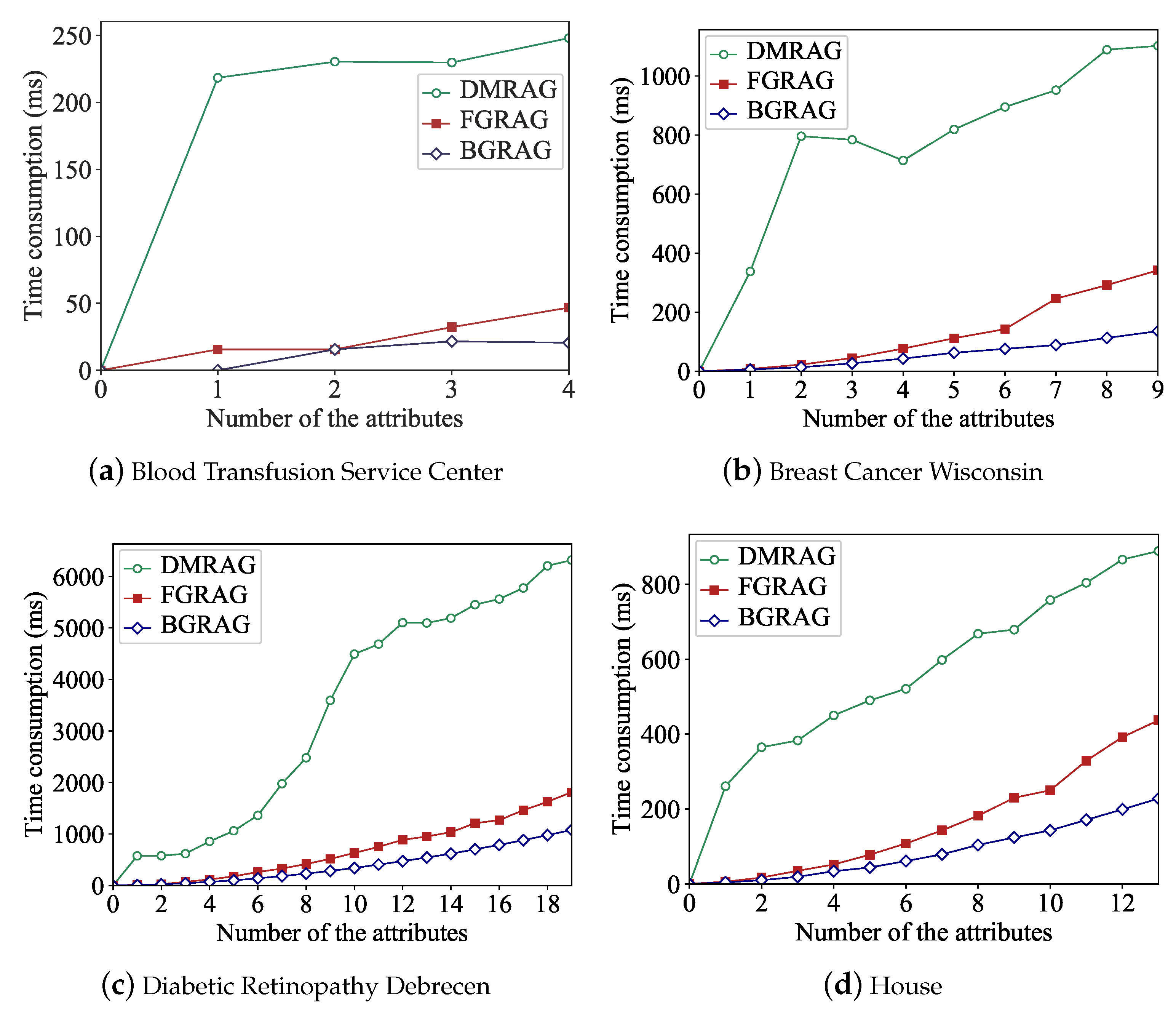
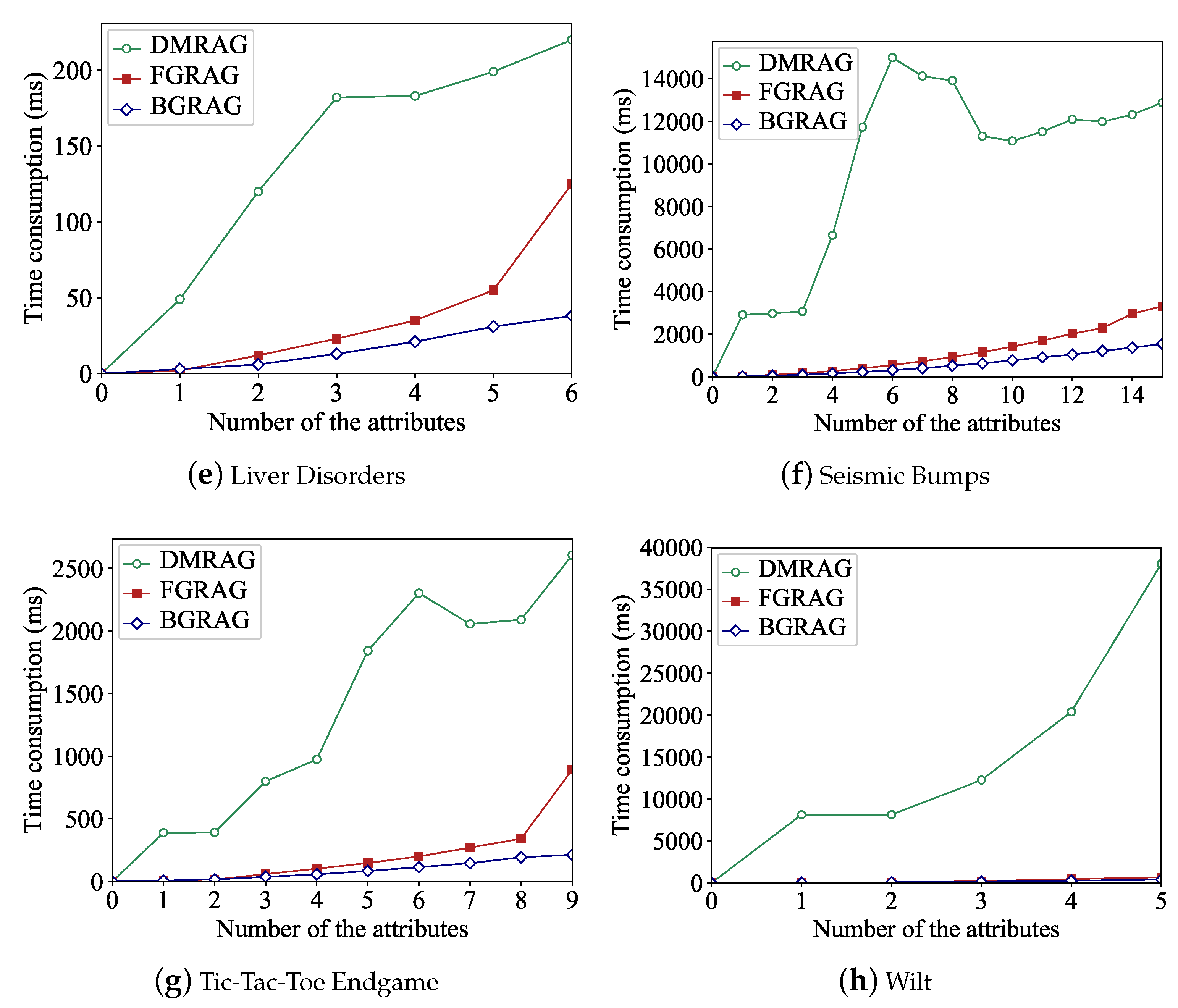
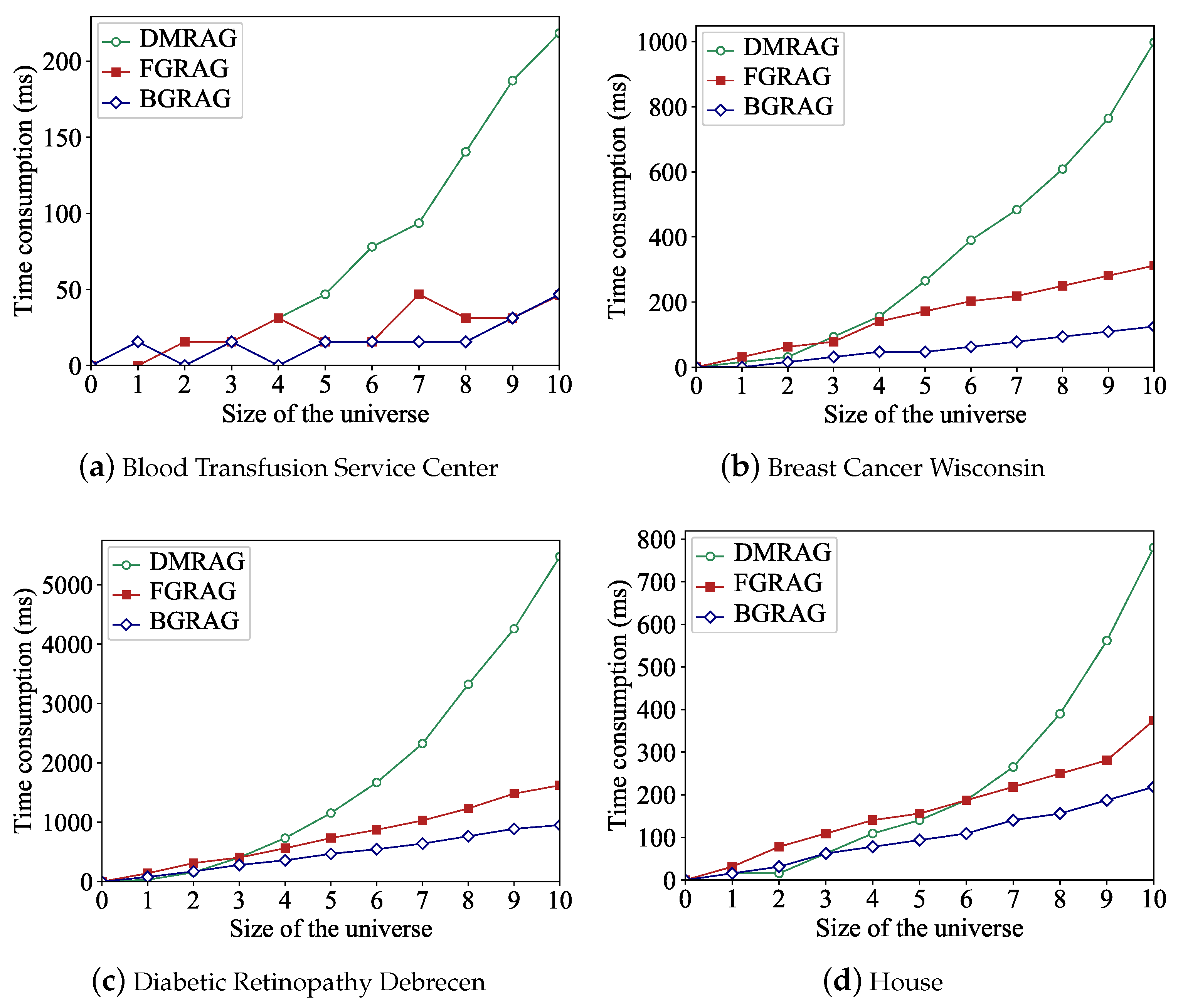
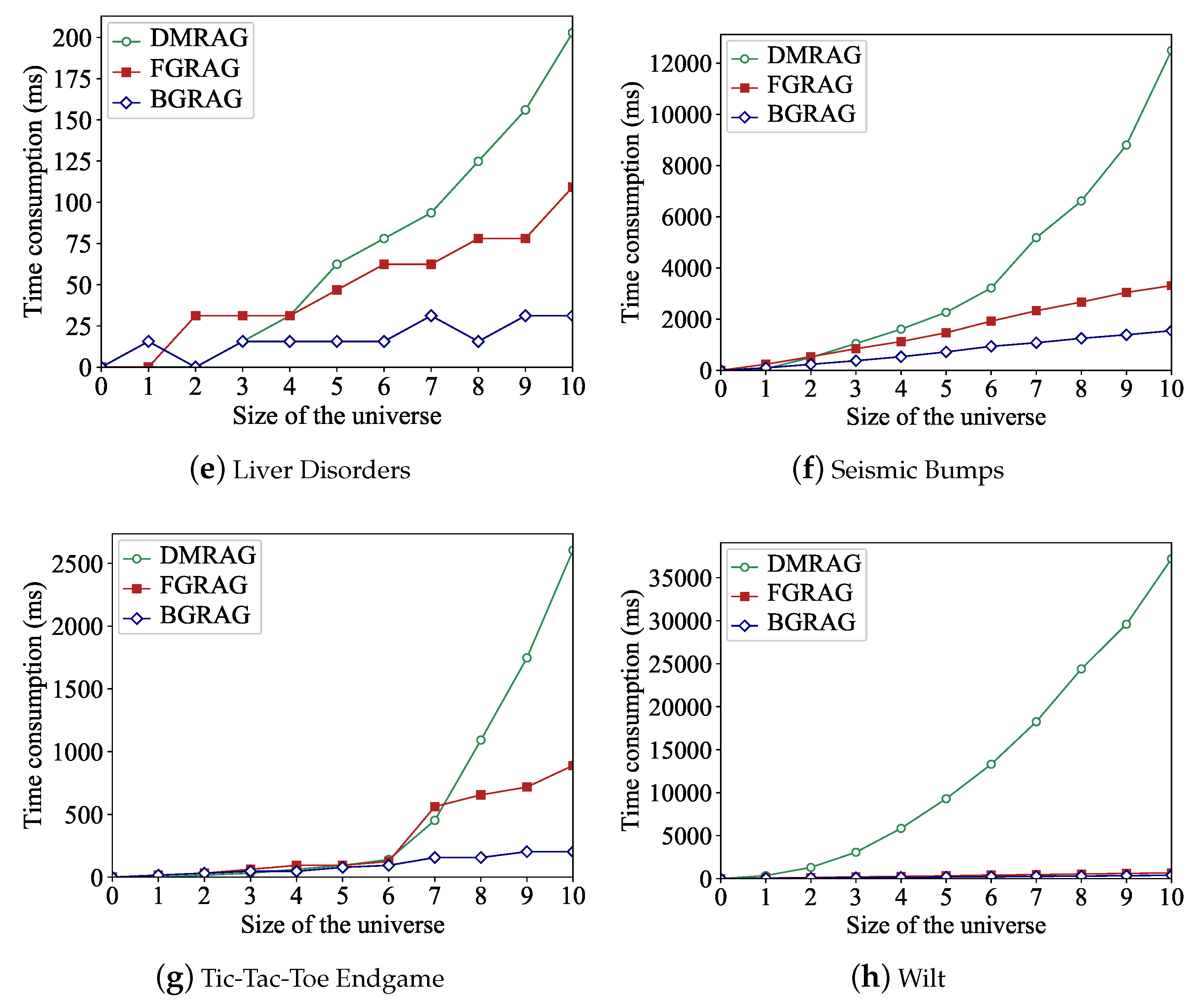
4.3. Efficiency of Proposed Attribute Reduction Algorithms

In this subsection, we will validate the efficiency of Algorithms 2 and 3. The running times of DMRAG, FGRAG, and BGRAG on the eight data sets are shown in

Table 4. Time consumption comparison of three algorithms.

Data Sets	Objects	Attributes	FGARG		BGARG		DMARG
			$|{\mathbf{Q}}_{\mathbf{1}}|$	t/ms	$|{\mathbf{Q}}_{\mathbf{2}}|$	t/ms	$|{\mathbf{Q}}_{\mathbf{3}}|$	t/ms
1	748	4	2	46	2	46	2	234
2	699	9	4	312	4	140	4.6	1029
3	1151	19	16	1687	16	1029	16	5678
4	506	13	11	405	11	202	11	920
5	345	6	5	109	5	46	5	218
6	2584	15	13	3123	13	1484	13	11,140
7	958	9	8	795	8	187	8	2888
8	4339	5	5	592	5	353	5	34,264

, where $\left|Q\right|$ denotes the number of the attributes in an attribute reduct Q. For DMRAG, $\left|Q\right|$ denotes the average number of the attributes of all reducts. Figure 2 and Figure 3 demonstrate the change trends of the running times of three algorithms (DMRAG, FGRAG, and BGRAG) with increasing size of data set. From Table 4, it is easy to see that the running time of DMRAG was the maximum among those of the three algorithms. In other words, both FGRAG and BGRAG were more efficient than DMRAG on the eight data sets. The running time of FGRAG (BGRAG) was much less than that of DMRAG. For example, DMRAG on the data set Tic-Tac-Toe Endgame (Number 7) took 2888 ms, whereas FGRAG and BGRAG took 795 ms and 187 ms, respectively. The running time of DMRAG was about 3 times and 15 times than those of FGRAG and BGRAG, respectively. From Table 4, it is clear that both FGRAG and BGRAG had higher efficiencies than DMRAG. Due to avoiding calculating the core, BGRAG was usually more efficient than FGRAG. In Table 4, the running time of BGRAG was the minimum among those of the three algorithms on seven data sets (namely, Breast Cancer Wisconsin, Diabetic Retinopathy Debrecen, House, Liver Disorders, Seismic Bumps, Tic-Tac-Toe Endgame, and Wilt).

Figure 2 indicates the change trends of the running times of three algorithms (DMRAG, FGRAG and BGRAG) with the number of the attributes increasing. In Figure 2a–h, the x-axis represents the number of the attributes, while the y-axis represents the time consumption of the three algorithms. The curves of FGRAG and BGRAG are totally under that of DMRAG. The running times of FGRAG and BGRAG were much less than that of DMRAG when dealing with the same amount of attributes. The curve of DMRAG rises rapidly when the number of the attributes increases, while those of FGRAG and BGRAG rise slowly. For example, in Figure 2a, the running time of DMRAG increased by 242 ms when the number of the attributes varied from 0 to 1, whereas the running times of FGRAG and BGRAG increased by only 10 and 6 ms, respectively. For Figure 2b, the running time of DMRAG increased by 796 ms when the number of the attributes varied from 0 to 2, whereas the running times of FGRAG and BGRAG increased by only 23 and 13 ms. It is obvious that Figure 2h is different from the others in Figure 2. The running time of FGRAG or BGRAG was much less than that of DMRAG when dealing with the same number of attributes. The differences between FGRAG and BGRAG in time consumption were much less than the differences between FGRAG (BGRAG) and DMRAG. Thus, the curves of FGRAG and BGRAG were relatively similar and very close to the x-axis. The running times of the three algorithms (DMRAG, FGRAG, and BGRAG) all increased with the number of the attributes. Nevertheless, the relationship between the number of the attributes and the running time was not strictly monotonic. For example, in Figure 2f, the running times of DMRAG were 14,126 ms and 13,907 ms, respectively, when the numbers of attributes were 7 and 8. The running time was reduced by 219 ms when the number of the attributes varied from 7 to 8. In Figure 2a–h, the curves of FGRAG and BGRAG are similar relatively. In the beginning, the differences between FGRAG and BGRAG are not visible. The differences between FGRAG and BGRAG became larger when the number of attributes increased. From Figure 2a–h, for the same number of the attributes, we can see that FGRAG (BGRAG) was more efficient than DMRAG and the efficiency of BGRAG was higher than FGRAG.

Figure 3 illustrates the change trends of the running times of three algorithms (DMRAG, FGRAG, and BGRAG) with increases in the size of the universe. For each sub-figure in Figure 3, the x-axis denotes size of the universe, while the y-axis denotes the time consumptions of the three algorithms. The size of the universe of each data set was divided into ten parts with equal size. The running times of the three algorithms (DMRAG, FGRAG, and BGRAG) increased with the size of the universe. The relationship between the size of the universe and the running time was also not monotonic strictly. For example, in Figure 3a, the running time of FGRAG was 31 ms when the size of the universe was 4, whereas the running time was 15 ms when the size of the universe was 5; that is, as the size of the universe increased from 4 to 5, the running time was reduced by 16 ms. From Figure 3, it can be easily observed that the gradient of the curve of DMRAG was bigger than that of FGRAG or BGRAG, generally. The running time of DMRAG increased significantly when the size of the universe increased, while the running time of FGRAG (or DMRAG) increased slowly. For Figure 3b, the running time of DMRAG increased by 842 ms when the size of the universe varied from 4 to 10, whereas the running times of FGRAG and BGRAG increased by only 171 ms and 78 ms, respectively. For Figure 3g, the running time of DMRAG increased by 2152 ms when the size of the universe varied from 7 to 10, whereas the running times of FGRAG and BGRAG increased by only 327 and 46 ms. In the beginning, the differences between DMRAG and FGRAG (or BGARG) were not obvious. The differences between DMRAG and FGRAG (or BGRAG) became larger when the size of the universe increased. For example, in Figure 3b, the running time of DMRAG increased significantly when the size of the universe was over 4. The differences between DMRAG and FGRAG (BGRAG) became larger than before. In Figure 3c, the differences between DMRAG and FGRAG (BGRAG) became larger when the size of the universe was over 4. It is easy to see that Figure 3h is different from the other subfigures in Figure 3. From Figure 3h, DMRAG needed far more time than FGRAG (BGARG) when dealing with the same sized universe. In other words, FGRAG (BGRAG) needed much less time than DMRAG. For example, DMRAG needed 13,306 ms, 24,398 ms, and 37,206 ms, when the size of the universe was 6, 8, and 10, respectively. Meanwhile, FGRAG needed 421 ms, 546 ms, and 670 ms, BGRAG needed 218 ms, 296 ms, and 390 ms. The differences between FGRAG and BGRAG, in terms of time consumption, were much less than the differences between FGRAG (BGRAG) and DMRAG. Thus, the curves of FGRAG and BGRAG are similar relatively and very close to x-axis. From Figure 3, it is profoundly visible that the efficiency of FGRAG (or BGRAG) was higher than that of DMRAG when dealing with the same size of the universe.

From the time complexity analyses of DMRAG, FGRAG, and BGRAG, the time complexity of DMRAG proposed by Miao et al. [12] was $O(m^{C_m^{⌈m/2⌉}}+m{n}^4)$, while the time complexities of FGRAG and BGRAG proposed in this paper were $O\left(m^{3}n\right)$ and $O\left(m^{2}n\right)$, where $m=\left|C\right|$ denotes the number of condition attributes and $n=\left|U\right|$ indicates the size of the universe (the number of objects). Therefore, in Figure 3, the running times of DMRAG, FGRAG, and BGRAG increased with the size of the universe generally. According to the time complexity of DMRAG, the running time of DMRAG was easily affected by the change of the number of objects. When the number of objects increased rapidly, the running time of DMRAG increased significantly. Therefore, in Figure 3, the curve of DMRAG rises distinctively when the size of the universe increases. The differences between FGRAG and BGRAG, in terms of time consumption, were much less than the differences between FGRAG (BGRAG) and DMRAG. The curves of FGRAG and BGRAG were relatively similar. In some cases, if the discernibility property for generalized decision preservation can be improved rapidly by adding the objects, the number of loops (or iterations) of FGRAG or BGRAG can be reduced correspondingly. Then, the running time of FGRAG or BGRAG decreases with the size of the universe increasing, in some cases. Thus, the relationship between the size of the universe and the running time was not strictly monotonic. For example, in Figure 3a, the running time of FGRAG was 46 ms when the size of the universe was 7, whereas the running time was 31 ms when the size of the universe was 8. In Figure 3a–h, due to avoiding calculating the core, BGRAG was more efficient than FGRAG in most cases.

5. Conclusions and Future Researches

Developing efficient algorithms for attribute reduction for decision systems is an important issue in many research fields, such as knowledge representation, multiple attribute decision making, and artificial intelligence. Discernibility matrix-based attribute reduction for generalized decision preservation has low computational efficiency and is intolerable for processing a large amount of data. To deal with this issue, a monotonic similarity measure for generalized decision preservation is introduced for attribute reduction. By using the proposed similarity measure, two types of heuristic attribute reduction algorithms (FGRAG and BGRAG) have been designed to obtain the reducts for generalized decision preservation in this paper. One is a forward attribute reduction algorithm based on the add-deleting strategy, the other is a backward attribute reduction algorithm based on the deleting strategy. Results of comparative experiments indicate that both FGRAG and BGRAG can significantly reduce the running time of attribute reduction, while retaining the generalized decision of each object in the universe.

The effectiveness of the proposed heuristic algorithms in machine learning and multi-attribute decision making is presented as follows: (1) In practical applications, the original data sets often contain redundant or irrelative attributes. These attributes may deteriorate the efficiency of learning algorithms. The proposed algorithms FGRAG and BGRAG can remove the redundant attributes from the original data sets quickly, and obtain the simplified data sets which only have indispensable attributes. These simplified data sets can reduce the cost of storage and improve the efficiency of learning algorithms, as well as providing an understandable approach for analyses of data set structures. (2) For a decision system, objects with the same condition attribute values may have different decision values. The rules with respect to these objects are referred to as uncertain rules. By the attribute reduction methods proposed in this paper, the possible decision values of each uncertain rule are left unchanged. Thus, the uncertain information in a decision system can be retained. Based on the reducts calculated by the proposed algorithms, simplified uncertain rules can be extracted from a decision system. These rules can be useful for multiple criteria decision making and decision conflict analyses.

Some future research directions are: (1) Attribute reduction for generalized decision preservation based on metaheuristic methods has not been proposed, so far. Based on studies of metaheuristic methods [25,27,29], attribute reduction for generalized decision preservation based on metaheuristic methods (i.e., bee colony or ant colony optimization) will be studied in the future. Some comparative experiments will be also conducted to verify that the proposed algorithms are effective. (2) The heuristic attribute reduction algorithms proposed in this paper are based on the equivalence relation and can be only used in classical Pawlak decision systems. However, in practical applications, there are many generalized decision systems, such as set-valued decision systems, interval-valued decision systems, and fuzzy decision systems. Heuristic attribute reduction algorithms for generalized decision preservation in generalized decision systems will be investigated in future studies.

References

1. Pawlak, Z. Rough sets. Int. J. Comput. Inf. Sci. 1982, 11, 341–356. [Google Scholar] [CrossRef]
2. Yao, Y.Y. Three-way decisions and cognitive computing. Cogn. Comput. 2016, 8, 543–554. [Google Scholar] [CrossRef]
3. Yao, Y.Y.; Zhou, B. Two Bayesian approaches to rough sets. Eur. J. Oper. Res. 2016, 251, 904–917. [Google Scholar] [CrossRef]
4. Qian, Y.H.; Liang, J.Y.; Yao, Y.Y.; Dang, C.Y. MGRS: A multi-granulation rough set. Inf. Sci. 2010, 180, 949–970. [Google Scholar] [CrossRef]
5. Zhang, N.; Li, B.Z.; Zhang, Z.X.; Guo, Y.Y. A quick algorithm for binary discernibility matrix simplification using deterministic finite automata. Information 2018, 9, 314. [Google Scholar] [CrossRef]
6. Wang, C.Z.; Qi, Y.L.; Shao, M.W.; Hu, Q.H.; Chen, D.G.; Qian, Y.H.; Lin, Y.J. A fitting model for feature selection with fuzzy rough sets. IEEE Trans. Fuzzy Syst. 2017, 25, 741–752. [Google Scholar] [CrossRef]
7. Lin, Y.J.; Hu, Q.H.; Liu, J.H.; Chen, J.K.; Duan, J. Multi-label feature selection based on neighborhood mutual information. Appl. Soft Comput. 2016, 38, 244–256. [Google Scholar] [CrossRef]
8. Skowron, A.; Rauszer, C. The discernibility matrices and functions in information systems. In Intelligent Decision Support: Handbook of Applications and Advances of the Rough Sets Theory; Słowiński, R., Ed.; Kluwer Academic Publishers: Dordrecht, The Netherlands, 1992; pp. 331–362. [Google Scholar]
9. Chebrolu, S.; Sanjeevi, S.G. Forward tentative selection with backward propagation of selection decision algorithm for attribute reduction in rough set theory. Int. J. -Reason.-Based Intell. Syst. 2015, 7, 221–243. [Google Scholar] [CrossRef]
10. Zhang, X.; Mei, C.L.; Chen, D.G.; Li, J.H. Feature selection in mixed data: a method using a novel fuzzy rough set-based information entropy. Pattern Recognit. 2016, 56, 1–15. [Google Scholar] [CrossRef]
11. Hu, X.H.; Cercone, N. Learning in relational databases: a rough set approach. Int. J. Comput. Intell. 1995, 11, 323–338. [Google Scholar] [CrossRef]
12. Miao, D.Q.; Zhao, Y.; Yao, Y.Y.; Li, H.; Xu, F. Relative reducts in consistent and inconsistent decision tables of the Pawlak rough set model. Inf. Sci. 2009, 179, 4140–4150. [Google Scholar] [CrossRef]
13. Kryszkiewicz, M. Rough set approach to incomplete information systems. Inf. Sci. 1998, 112, 39–49. [Google Scholar] [CrossRef]
14. Miao, D.Q.; Hu, G.R. A heuristic algorithm for reduction of knowledge. J. Comput. Res. Dev. 1999, 36, 681–684. [Google Scholar]
15. Zhang, W.X.; Mi, J.S. Knowledge reductions in inconsistent information systems. Chin. J. Comput. 2003, 261, 12–18. [Google Scholar]
16. Guan, Y.Y.; Wang, H.K.; Wang, Y.; Yang, F. Attribute reduction and optimal decision rules acquisition for continuous valued information systems. Inf. Sci. 2009, 179, 2974–2984. [Google Scholar] [CrossRef]
17. Xu, W.H.; Li, Y.; Liao, X.W. Approaches to attribute reductions based on rough set and matrix computation in consistent order information systems. Knowl.-Based Syst. 2012, 27, 78–91. [Google Scholar] [CrossRef]
18. Yang, X.B.; Qi, Y.; Yu, D.J.; Yu, H.L.; Yang, J.Y. α-Dominance relation and rough sets in interval-valued information systems. Inf. Sci. 2015, 294, 334–347. [Google Scholar] [CrossRef]
19. Du, W.S.; Hu, B.Q. Dominance-based rough fuzzy set approach and its application to rule induction. Eur. J. Oper. Res. 2017, 261, 690–703. [Google Scholar] [CrossRef]
20. Zhou, J.; Miao, D.Q.; Pedrycz, W.; Zhang, H.Y. Analysis of alternative objective functions for attribute reduction in complete decision tables. Soft Comput. 2011, 15, 1601–1616. [Google Scholar] [CrossRef]
21. Li, H.; Li, D.Y.; Zhai, Y.H.; Wang, S.G.; Zhang, J. A novel attribute reduction approach for multi-label data based on rough set theory. Inf. Sci. 2016, 367–368, 827–847. [Google Scholar] [CrossRef]
22. Du, W.S.; Hu, B.Q. A fast heuristic attribute reduction approach to ordered decision systems. Eur. J. Oper. Res. 2018, 264, 440–452. [Google Scholar] [CrossRef]
23. Wang, F.; Liang, J.Y.; Dang, C.Y. Attribute reduction for dynamic data sets. Appl. Soft Comput. 2013, 13, 676–689. [Google Scholar] [CrossRef]
24. Jensen, R. Combining Rough and Fuzzy Sets for Feature Selection. Ph.D. Thesis, University Of Edinburgh, Edinburgh, UK, 2005. [Google Scholar]
25. Chebrolu, S.; Sanjeevi, S.G. Attribute reduction on real-valued data in rough set theory using hybrid artificial bee colony: Extended FTSBPSD algorithm. Soft Comput. 2017, 21, 7543–7569. [Google Scholar] [CrossRef]
26. Chebrolu, S.; Sanjeevi, S.G. Attribute reduction in decision-theoretic rough set models using genetic algorithm. In Proceedings of the International Conference on Swarm, Evolutionary, and Memetic Computing (LNCS 7076), Visakhapatnam, India, 19–21 December 2011; pp. 307–314. [Google Scholar]
27. Chebrolu, S.; Sanjeevi, S.G. Attribute reduction on continuous data in rough set theory using ant colony optimization metaheuristic. In Proceedings of the Third International Symposiumon Women in Computing and Informatics, Kochi, India, 10–13 August 2015; pp. 17–24. [Google Scholar]
28. Chebrolu, S.; Sanjeevi, S.G. Attribute reduction in decision-theoretic rough set model using particle swarm optimization with the threshold parameters determined using LMS training rule. Procedia Comput. Sci. 2015, 57, 527–536. [Google Scholar] [CrossRef]
29. Chen, Y.M.; Miao, D.Q.; Wang, R.Z. A rough set approach to feature selection based on ant colony optimization. Pattern Recognit. Lett. 2010, 31, 226–233. [Google Scholar] [CrossRef]
30. Min, F.; Zhang, Z.H.; Dong, J. Ant colony optimization with partial-complete searching for attribute reduction. J. Comput. Sci. 2018, 25, 170–182. [Google Scholar] [CrossRef]
31. Leung, Y.; Li, D.Y. Maximal consistent block technique for rule acquisition in incomplete information systems. Inf. Sci. 2003, 153, 85–106. [Google Scholar] [CrossRef]
32. Miao, D.Q.; Zhang, N.; Yue, X.D. Knowledge reduction in interval-valued information systems. In Proceedings of the 8th International Conference on Cognitive Informatics, Hongkong, China, 15–17 June 2009; pp. 320–327. [Google Scholar]
33. Liu, G.L.; Hua, Z.; Zou, J.Y. Local attribute reductions for decision tables. Inf. Sci. 2018, 179, 204–217. [Google Scholar] [CrossRef]
34. Qian, Y.H.; Liang, J.Y.; Pedrycz, W.; Dang, C.Y. Positive approximation: an accelarator for attribute reduction in rough set thoery. Artifical Intell. 2010, 174, 595–618. [Google Scholar] [CrossRef]
35. Dai, J.H.; Hu, H.; Zheng, G.J.; Hu, Q.H.; Han, H.F.; Shi, H. Attribute reduction in interval-valued information systems based on information entropies. Front. Inf. Technol. Electron. Eng. 2016, 17, 919–928. [Google Scholar] [CrossRef]
36. Jia, X.Y.; Liao, W.H.; Tang, Z.M.; Shang, L. Minimum cost attribute reduction in decision-theoretic rough set models. Inf. Sci. 2013, 219, 151–167. [Google Scholar] [CrossRef]
37. Cheng, Y.; Zheng, Z.R.; Wang, J.; Yang, L.; Wan, S.H. Attribute reduction based on genetic algorithm for the coevolution of meteorological data in the industrial internet of things. Wirel. Commun. Mob. Comput. 2019, 2019, 3525347. [Google Scholar] [CrossRef]
38. Li, M.; Shang, C.X.; Feng, S.Z.; Fan, J.P. Quick attribute reduction in inconsistent decision tables. Inf. Sci. 2014, 254, 155–180. [Google Scholar] [CrossRef]
39. Wang, C.Z.; Shao, M.W.; Sun, B.Z.; Hu, Q.H. An improved attribute reduction scheme with covering based rough sets. Appl. Soft Comput. 2015, 26, 235–243. [Google Scholar] [CrossRef]
40. Wang, G.Y.; Yu, H.; Yang, D.C. Decision table reduction based on conditional information entropy. Chin. J. Comput. 2002, 25, 759–766. [Google Scholar]
41. Gao, C.; Lai, Z.H.; Zhou, J.; Zhao, C.R.; Miao, D.Q. Maximum decision entropy-based attribute reduction in decision-theoretic rough set model. Knowl.-Based Syst. 2018, 143, 179–191. [Google Scholar] [CrossRef]
Figure 1. Monotonicity of the similarity degree.
Applsci 09 02841 g001
Figure 2. Time consumption comparison with the attributes increasing.
Applsci 09 02841 g002aApplsci 09 02841 g002b
Figure 3. Time consumption comparison with the universe increasing.
Applsci 09 02841 g003aApplsci 09 02841 g003b