Structural Reliability Estimation with Participatory Sensing and Mobile Cyber-Physical Structural Health Monitoring Systems

Abstract

With the help of community participants, smartphones can become useful wireless sensor network (WSN) components, form a self-governing structural health monitoring (SHM) system, and merge structural mechanics with participatory sensing and server computing. This paper presents a methodology and framework of such a cyber-physical system (CPS) that generates a bridge finite element model (FEM) integrated with vibration measurements from smartphone WSNs and centralized/distributed computational facilities, then assesses structural reliability based on updated FEMs. Structural vibration data obtained from smartphones are processed on a server to identify modal frequencies of an existing bridge. Without design drawings and supportive documentation but field measurements and observations, FEM of the bridge is drafted with uncertainties in the structural mass, stiffness, and boundary conditions (BCs). Then, 2700 FEMs are autonomously generated, and the baseline FEM is updated by minimizing the error between the crowdsourcing-based modal identification results and the FEM analysis. Furthermore, using 151 strong ground motion records from databases, the bridge response time history simulations are conducted to obtain displacement demand distribution. Finally, based on reference performance criteria, structural reliability of the bridge is estimated. Integrating the cyber (FEM analysis) and the physical (the bridge structure and measured vibration characteristics) worlds, this crowdsourcing-based CPS can provide a powerful tool for supporting rapid, remote, autonomous, and objective infrastructure-related decision-making. This study presents a new example of the emerging fourth industrial revolution from structural engineering and SHM perspective.

1. Introduction

Deriving economical, sustainable, and practical solutions without a compromise in infrastructure safety and integrity is a broad challenge in civil and structural engineering disciplines. The unpredictable nature of hazardous events combined with limited resources lead the current practice to inherit performance-based criteria in structural design and evaluation. Therefore, controlling the extent of structural damage rather than exclusively avoiding it, is the trending principle in up-to-date engineering codes and regulations [1,2].

Observing the changes in vibration characteristics of structures with the state-of-the-art sensing and processing tools, structural health monitoring (SHM) technologies attract significant attention in research and industry in the last three decades [3,4,5,6]. On the other hand; instrumentation, cabling, operation, and maintenance of SHM systems require labor work, knowhow, and financing; declining the growth rate of SHM use in practice. Especially in the past decade, these drawbacks lead researchers to focus on innovative methods such as noncontact vibration measurement techniques [7,8,9], wireless sensor network (WSN) and distributed sensor network (DSN) systems [10,11,12,13,14,15,16], as well as smart [17,18,19], mobile [20,21,22,23], and multisensory [24,25,26,27] sensing platforms. Eventually, smartphones are adopted into SHM such that their built-in sensors, operating systems, computation, and wireless communication capabilities can perform as structural vibration measurement devices [28,29,30,31].

The authors’ previous works present the first vibration-based SHM system (CS4SHM) using crowdsourcing power [32] and offer multisensory solutions to citizen-induced errors by considering spatiotemporal [33] and directional [34] uncertainties. Without any prior engineering education and background, citizens as uncontrolled SHM device operators can provide a central server system with ubiquitous vibration data. The acquired data is autonomously processed for modal identification which is an important indicator of structural vibration characteristics. Unlike conventional SHM systems, CS4SHM points out unorthodox monitoring issues which are concurrently discussed in the upcoming technological boom “Industry 4.0”, the latter phase of digital revolution [35,36]. Collecting the distributed crowd sensed information through a central server and conducting modal identification autonomously, civil infrastructures as physical objects are connected with server-side computing in a massive scale forming a CPS [37,38,39,40,41], or in some cases, an Internet of Things system [42,43,44,45]. This highlights a significant potential to evolve from pure theoretical structural response simulation (FEM) to experiment-aided and calibrated models (model updating) in massive scales. In other words, with the help of autonomous, connected, scalable cyber networks; citizen-engaged sensing; digital (FEM predictions) and physical (field measurements) civil infrastructure representations; monitoring systems can be adopted to the upcoming technological innovations.

Aforementioned hybrid models can be used for large-volume analysis to retrieve quick evaluation of structural status. This can be performed by utilizing the modal identification results, calibrating mathematical models, and obtaining the probabilistic failure distribution under a wide range of strong ground motions. Eventually, using identification results as model calibration tools, civil infrastructures’ seismic response and structural reliability can be estimated [46,47] to provide the decision makers with the necessary information.

This study presents the last section of a PhD dissertation dedicated to cyber-physical system applications from structural engineering perspective [48]. The paper extends the outcomes of a crowdsourcing-based modal identification platform by modifying FEMs constructed with limited information. FEMs as cyber representatives of building behavior are updated to minimize the error between the simulated models and the identification results obtained from the “physical objects”. Then, the updated models, which represent the actual vibration characteristics to a better extent, are used to simulate structural response under different earthquake motion scenarios. Finally, collecting the simulation results obtained from numerous time history analyses, the demand distribution is evaluated according to the exemplary code and regulation criteria. To summarize, the developed platform presents an innovative mobile CPS by converting the very initial physical vibrations into highly abstracted decision-making information (i.e., service close, retrofitting, and reconstruction) through a digital and multiphase mathematical information processing framework.

Section 2 discusses the experimental and theoretical phases of the methodology followed throughout the study. These phases include information about the testbed bridge structure, the CPS adaptation, model updating, and reliability estimation methodologies. Section 3 presents the application to the testbed and presents the monitoring results including objective function minimization and determination of structural reliability. Finally, Section 4 reviews the overall work, introduces the future goals, and highlights the concluding remarks.

2. Materials and Methods

The methodology presented in this study connects the experimental data obtained from civil infrastructures with the advanced mathematical modeling and analysis procedures. The following subsections introduce the testbed structure, modal identification, FEM updating, and reliability estimation processes as a CPS framework. From sensing to decision making, Figure 1 represents an idealized cyber-physical information processing scheme, with a comparison of the current CS4SHM system. The up-to-date platform is capable of receiving vibration measurements from citizens and conduct modal identification on the server-side. Then, the identification results are collected to set the reference modal analysis values for FEM updating and reliability estimation procedures. These phases are currently conducted through a scripted Matlab and OpenSees [49] loop, and the ultimate goal is to handle these cyber procedures through cloud computing. Nevertheless, in both cases, the decision makers can be provided with the quantitative information regarding structural status. Depending on the changes made to the structural system, the effects will be reflected on the future vibration characteristics which completes the cyclic information processing scheme.

It should be noted that the probabilistic nature given here is mainly concentrated on input ground motion and FE model updating. In fact, the effect of participatory sensing is an indispensable aspect of the system proposed in this paper since citizen engagement brings numerous uncertainties into the measurements. Previously, it has been shown that actual crowdsourcing results (results from uncontrolled citizens) matched well with the reference identification results [32]. These uncertainties are extensively studied in [48] including spatiotemporal variation of a citizen sensor [33], phone orientation which is subjected to change before, during, and after the measurements [34], and biomechanical distortions caused by human nature [50]. Therefore, in this paper, the main focus is on uncertainties induced by ground motions and FE model parameters.

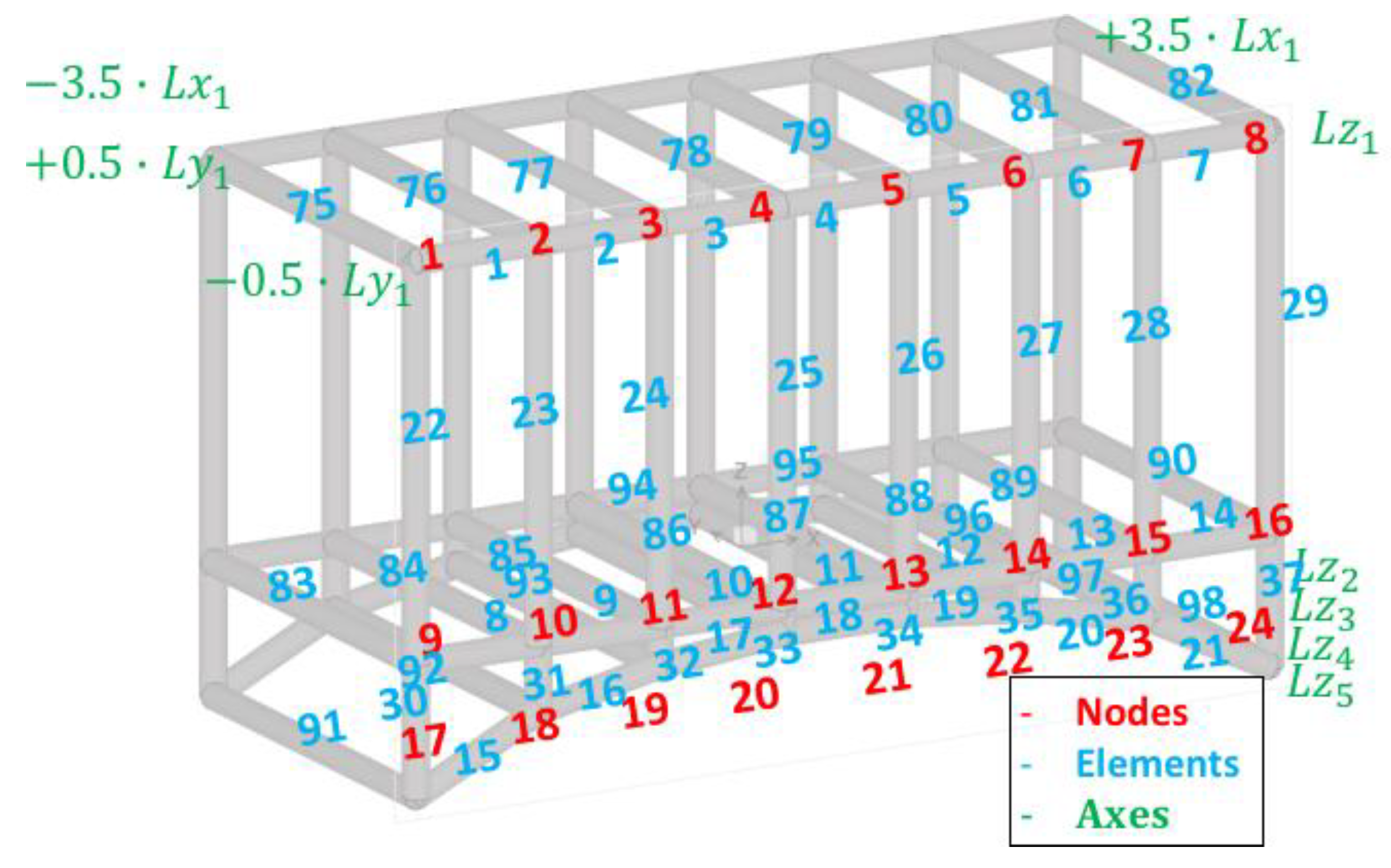
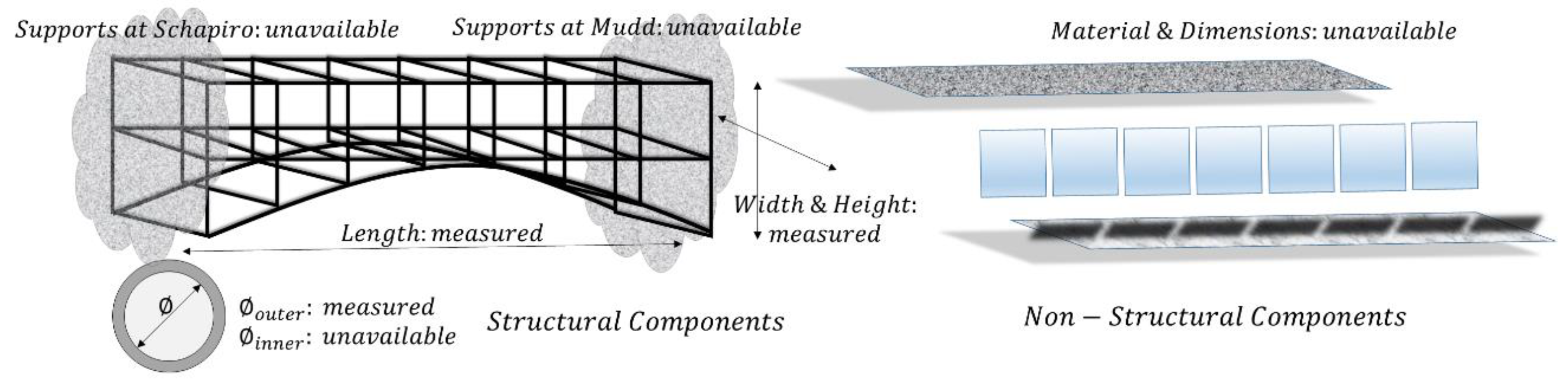
2.1. Testbed Structure

In order to select a testbed structure with crowdsourcing potential, a link bridge with pedestrian access is implemented. The bridge is a steel frame structure connecting two adjacent buildings in Columbia University Morningside Campus, namely, Mudd and Schapiro Buildings. Mudd Schapiro Link Bridge, shown in Figure 2, is an arch structure with rigid connections spanning approximately 10.5 m. Using the known dimensions of a window and a vision-based scaling procedure, the structural dimensions are approximated without any supplementary documents and design drawings. These dimensions constitute the baseline for the mathematical model, which later on, will be updated with the information from crowdsourced vibration data.

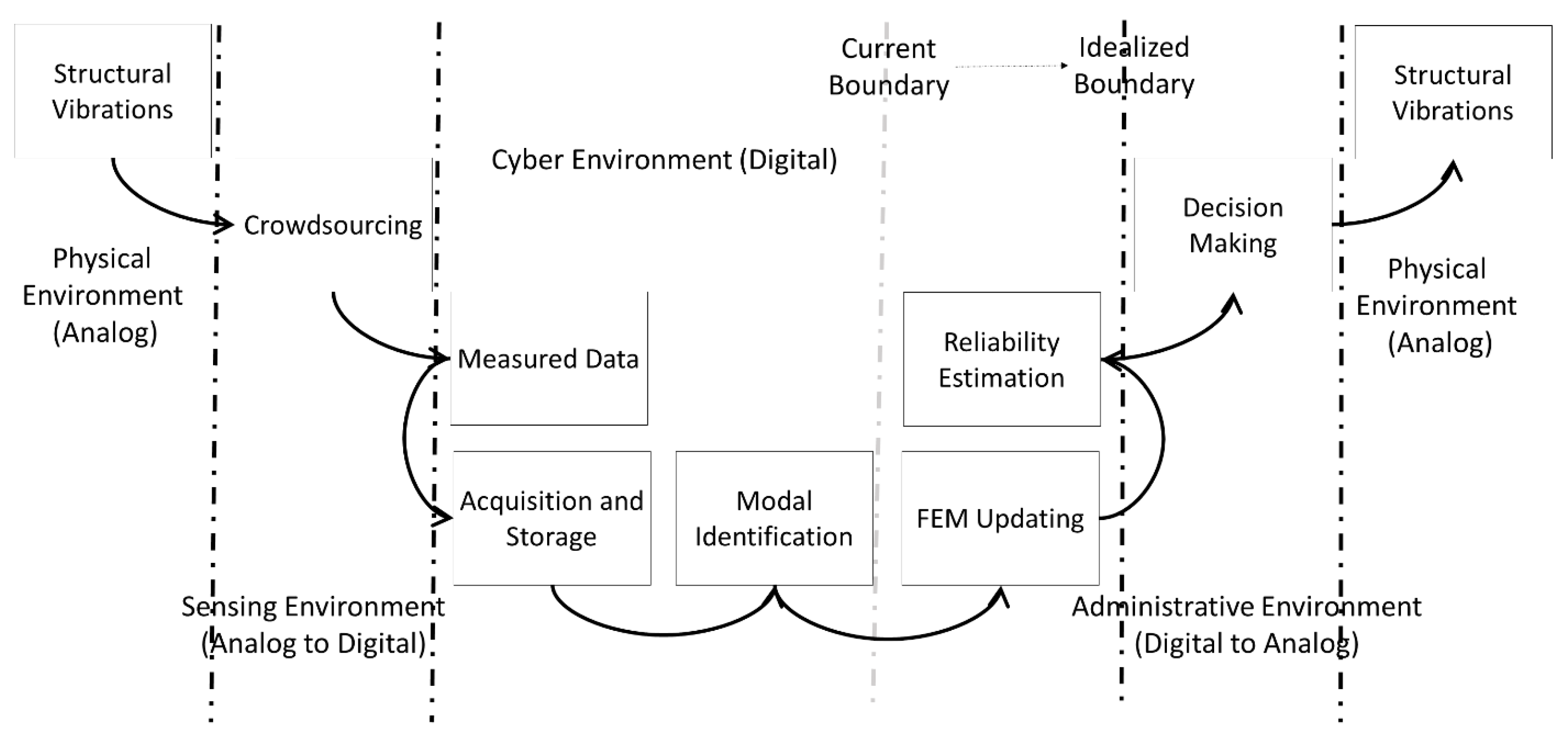
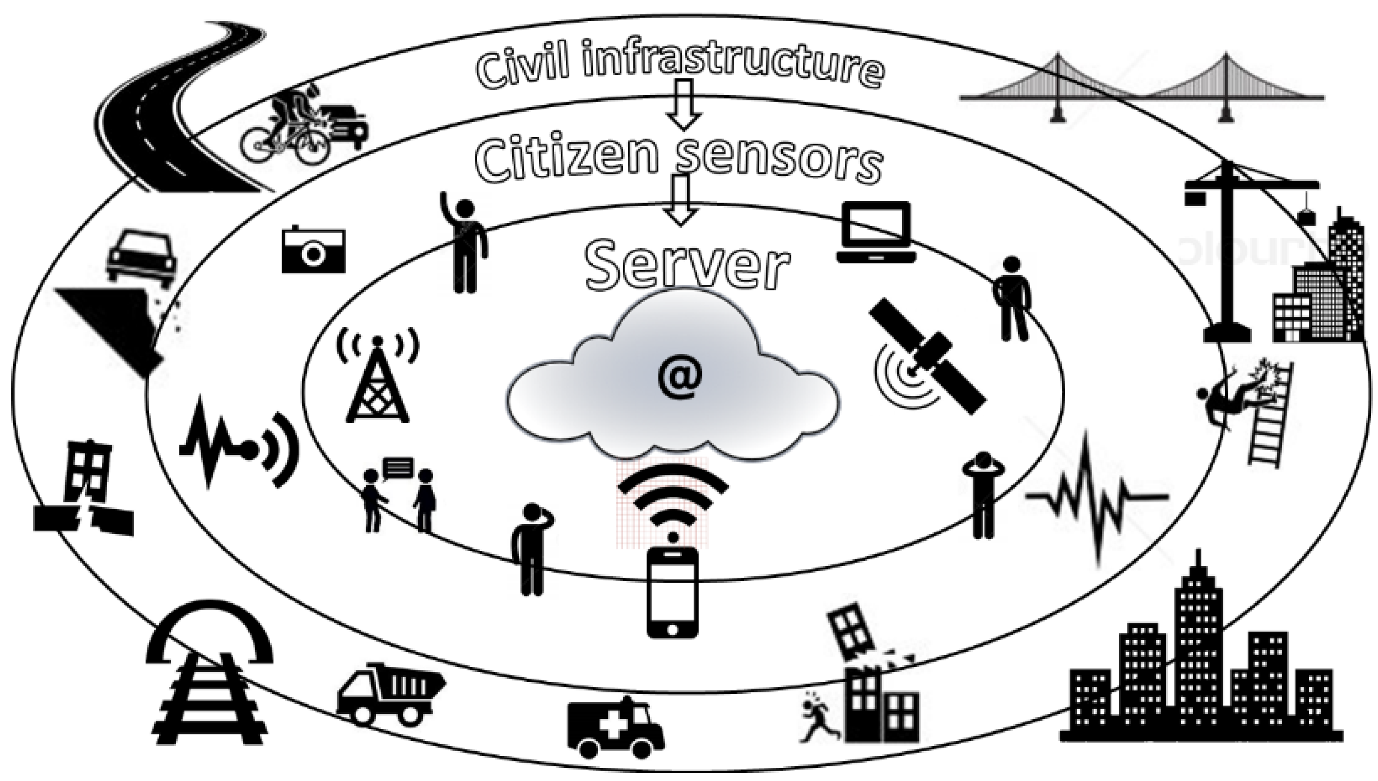
2.2. Cyber-Physical System

As a new emerging technology, CPSs attract significant attention from numerous research and industry fields in the last decade. The link and coordination between physical objects and computational resources set the fundamental system goal, which in return, brings different disciplines such as computer, control, electronic, and mechanical systems together [51]. Combining multilayered computer architectures [52] with embedded systems, sensors and control [53], or expanding WSNs to take action in the physical world [54], CPSs present a diverse interpretation of the up-to-date existing technologies.

The overall motivation of the CPS platform presented in this study is to connect the physical, cyber, and sensor system objects through a multilayered information processing SHM framework. The physical object formulated in this scheme is the bridge structure which represents the outer layer of the developed CPS system, as shown in Figure 3. The physical parameter of interest is the bridge vibrations, which can be gathered by smartphone accelerometers with the help of pedestrian volunteers. Moreover, the sensing process is enhanced by the hybrid foundation of pedestrians and sensors, composing the citizen sensor layer. Eventually, the bridge vibrations sensed by smartphone accelerometers are submitted to the server where the signal processing and data analytics take place. With the help of the cloud-based acceleration record manager system, which is the innermost layer, the vibration data can be stored, viewed, reprocessed, and their results can directly be extracted by the system administrators. Interconnecting these components successively forms the two core elements (sensor networks and application platforms) with transactions (sensing and knowledge) of a typical CPS and produce the actuation information with intelligent decision systems to complete the cyber-physical loop [39]. To summarize, citizen sensors provide the binding components of the smartphone-based SHM network by integrating the civil infrastructure with the cloud services, and the numerical representations of the bridge (FEMs) can be fed with the actual bridge response through the cyber-physical SHM system phases.

Formerly, the bridge is registered to the CS4SHM online server system and database to store, process, and monitor its structural vibrations. An iOS application is developed as a data acquisition interface to enable smartphone users gather vibration data from the bridge and submit it to the server. Pedestrians with bridge access are assigned as the test group and submitted 135 vibration measurements in total. The data is processed through the online server system, and modal identification results are recorded. These identification results can be used to calibrate the mathematical model of the bridge by following the FEM updating procedure. Figure 4 shows an exemplary citizen sample in the time and the frequency domains. Based on the whole set of submission records, first, second, and third modal frequencies are identified in [32] as 8.5, 19, and 30 Hz, respectively.

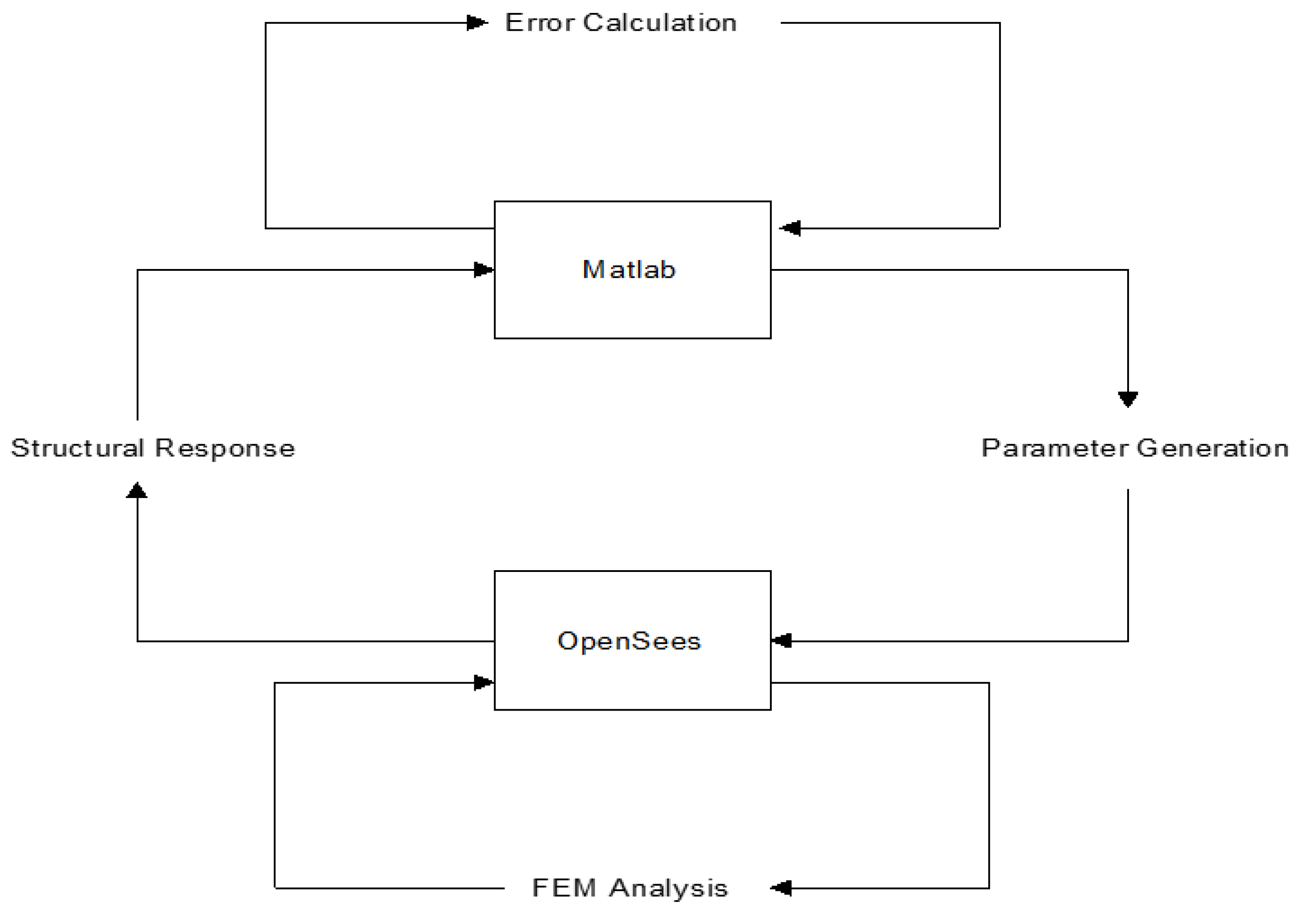
2.3. Finite Element Model Updating

In order to predict the structural response accurately, the available information should be effectively used such that FEM parameters can be determined to the best extent. In this modeling example, the design drawings and material properties are unavailable, therefore, the initial FEM is based on site observations and estimations. The observations include the length and the outer diameter of structural members by scaling the pixel values with respect to the known dimensions (i.e., window size). Although the outer diameter can be determined using bridge photographs, the cross-sectional thickness or the inner diameter is unknown. Likewise, support restraints are set as uncertain parameters with possible realizations such as fixed, pinned, or roller. Other than these, contribution of the nonstructural components is difficult to estimate, therefore, mass sources are assigned based on crude assumptions. The analysis primarily considers displacement demand in the vertical direction which is influential on glass façade safety, and the paper presents time history analysis results in z-direction. The model consists of 48 nodes and 98 beam-column elements. Figure 5 shows the node and element tags for the baseline model.

Figure 6 shows the modeling uncertainties taking place without the necessary documentation. To summarize, tubular structural member section dimensions, distributed mass due to non-structural components, and support restraints all contribute to the modeling uncertainties and will be determined throughout the FEM updating process.

The proposed FEM updating method consists of generating a large number of models changing in uncertain parameters, comparing the modal analysis results of each FEM with the experimental data, and selecting the model which minimizes the error between the simulation (model) and the reality (identification). In order to establish an autonomous parameter study and FEM updating procedure, an OpenSees-Matlab integration loop is pursued. Specifically, OpenSees scripts are simultaneously generated, run, and evaluated by a controller Matlab code. As mentioned previously, three different parameters are selected to create different FEM batches. These are the boundary conditions, element stiffness values, and nodal masses, respectively. For each boundary condition combination changing in fixity definitions, a set of models with varying stiffness and mass values are generated. Each of the model batches are evaluated according to the difference between the first, second, and the third FEM and identification results. This is conducted by developing an objective function quantifying the error between a model and the reference modal parameter values.

In the former studies, the authors adopted Least Square Method (LSM) to formulate the objective function [46,47] whereas different approaches are present in the literature [55,56], in this study, the objective function is structured in terms of error between the simulation and the experimental results and multiplication of multiple modal parameter errors. To specify, the objective function, which is a function of the support restraints, stiffness and mass distributions, is formulated as

$$\mathrm{Obj}\left(\mathrm{BC},\mathrm{K},\mathrm{M}\right)={\displaystyle \prod }_{\mathrm{mode}=1}^3\left(\left|{\mathrm{f}}_{\mathrm{mode}\mathrm{FEM}}-{\mathrm{f}}_{\mathrm{mode}\mathrm{EXP}}\right|/{\mathrm{f}}_{\mathrm{mode}\mathrm{EXP}}\right)$$

where BC, K, M represent changing FEM parameters such as boundary condition (BC), member stiffness, and mass values, respectively. Each boundary condition, stiffness, and mass combination corresponds to a different set of first, second, and third modal frequencies represented with ${\mathrm{f}}_{\mathrm{mode}\mathrm{FEM}}$ term, and the model accuracy is determined based on the deviation from experimental values represented with ${\mathrm{f}}_{\mathrm{mode}\mathrm{EXP}}$. At the end of the loop analyses, the optimal model which minimizes the error between the simulated and identified values becomes the updated model. Afterwards, this model can be used as a baseline for seismic response simulations and reliability estimation.

To summarize the updating process, Figure 7 shows the relationship between the OpenSees and Matlab platforms. The finite element model generation and updating process consists of two integrated platforms which are Matlab and OpenSees. Matlab basically works as a commander, it manipulates finite element parameters stored in OpenSees script files and utilizes the time history analysis outputs from OpenSees. OpenSees functions as a script-based modeling program (suitable for automated batch analysis), is used to conduct modal analysis or time history analysis and is controlled by Matlab. The two pieces of software work in harmony to conduct a large number of automated analysis with a common baseline model but differences in updated parameters.

2.4. Structural Reliability Estimation

In the authors’ previous studies, SHM-integrated reliability estimation is performed by generating fragility curves of different performance levels taking peak ground acceleration (PGA) as the random variable [46,47]. This method can result in high computational cost as the number of available seismic ground motions increases. Compatible with the smartphone-based identification procedure presented in this study, it is expected that ground motion demands under a seismic event can be determined by a dense seismic network composed of smartphone seismometers [57]. Besides, as the number of input ground motions increases like in a mobile CPS scenario, accuracy of the fragility curve parameters may run into obstacles due to truncation and round-off errors. Therefore, in this study, the probabilistic structural response is directly obtained from log-normal distribution of the time history analysis results. Damping term in equation of motion is modeled with Rayleigh Damping where the associated matrix is a combination of stiffness and mass proportional damping. Alpha and beta coefficients are determined based on 2% damping ratio at first and third modes.

For each ground motion taken from the 1994 Northridge Earthquake, a time history analysis is conducted, and the simulated response is obtained. Because the bridge considered in this study is a high frequency structure compared to the low frequency character of Northridge Earthquake records, it is assumed that the structure undergoes linear behavior and its response can be simulated with linear time history analysis. In this case, secondary performance indicators such as maximum drift or displacement become important as they are decisive in the basic engineering mechanics assumptions. Therefore, the response from each seismic event is collected in terms of maximum deflection and finally, the distribution demand under the given set of earthquakes is obtained. Looking at the distribution demand as well as the reference code and regulation criteria, it can be predicted whether the structural response will exceed certain performance thresholds. In conclusion, with the proposed reliability estimation framework, the high computational cost of fragility curve development is swapped with a simpler approximation, provided that the ground motion response distribution matches well with log-normal type distribution features.

It should be noted that 1994 Northridge Earthquake records perform as an exemplary dataset thanks to the high number of stations and well-distributed strong motion parameters, however, they do not necessarily mirror testbed site conditions presented in this paper. In other words, they are referred for demonstration purposes. In contrast with California, seismicity in the state of New York possesses a lower risk and lacks a comprehensive dataset available to public. However, in the event of ground motion record lack, synthetic ground motions can be generated for a particular site which has designated earthquake spectra [58]. What is more, in a futuristic scenario where there is seismic activity in urban areas, smartphones have shown feasible performance as low-cost seismometers which can be used to detect input ground motion imposed on civil infrastructure [57].

Considering the similar geometry and accordingly similar dynamic behavior of adjacent buildings, out of phase motions are not taken as a primary source of seismic damage. Therefore, forcing function at the boundaries are assumed to be uniform rather than multi-support excitation. It should be noted that changes in boundary conditions can also be monitored with the help of the proposed model updating procedure. Besides, given that the bridge lays on top of campus area with complete occupant access, glass façade integrity can also add additional life safety concerns in case of a seismic event. To incorporate that, vertical displacement behavior is taken as an exemplary performance parameter for reliability analysis.

3. Results and Discussion

Following the outline presented in the methodology, the testbed bridge data is used for modal identification, FEM updating, and reliability estimation with the updated model. The results obtained throughout the analysis are presented with two subsections discussing objective function minimization (FEM Updating) and simulation of seismic response (Reliability Estimation), respectively.

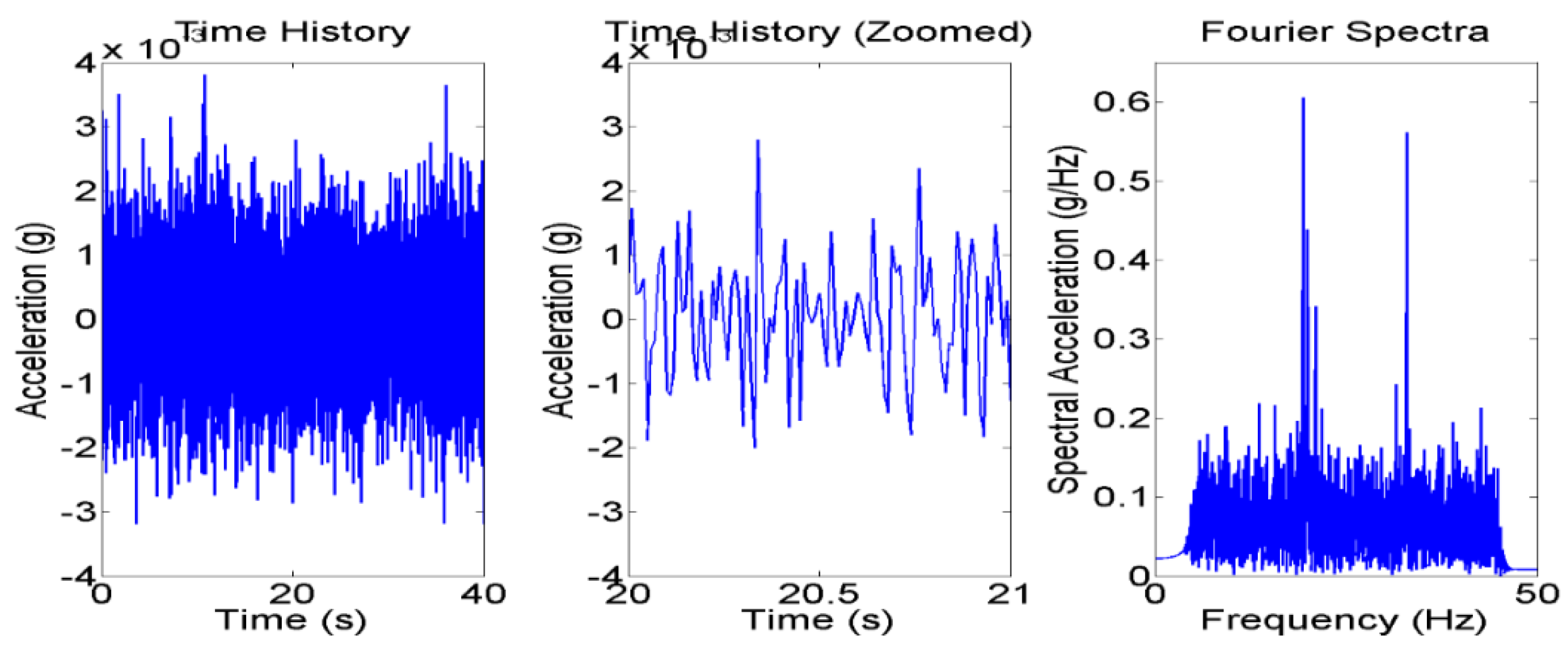
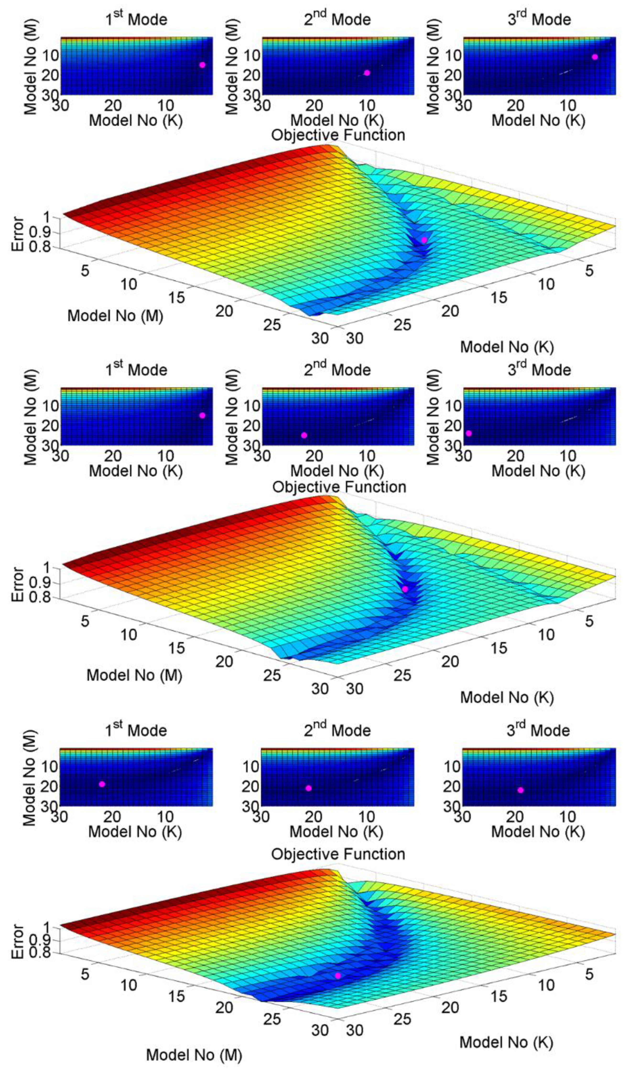
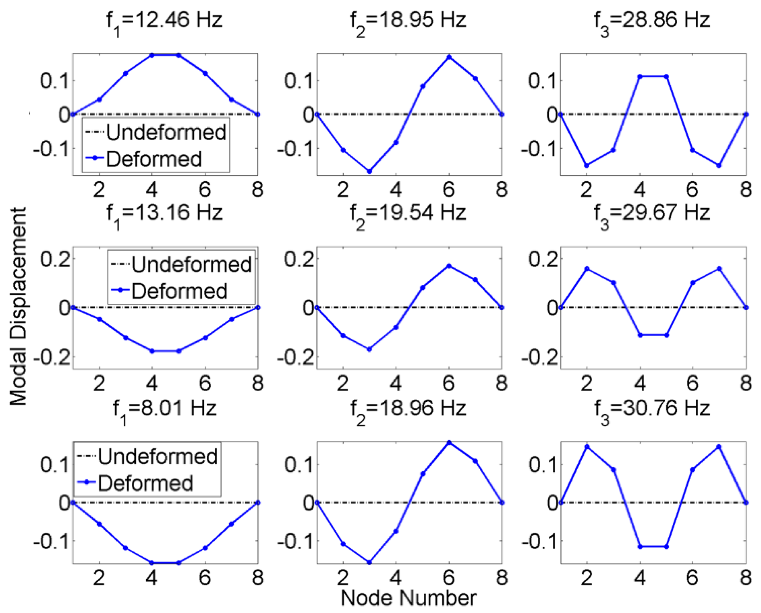
3.1. Objective Function Minimization

In order to predict the structural performance under hazardous events accurately, a well-tuned baseline model is essential. With limited modeling information due to lack of design drawings and reports, an approximate model may deviate from the actual behavior of the structure. Based on the field observations, mass estimations, and fixed BCs, modal analysis results of the initial non-updated model are 8.98, 14.41, and 22.05 Hz for first, second, and third modes, respectively. Comparing these results with the actual dynamic response obtained from the identification results, one can see there is a significant mismatch in second and third modes. Therefore, such modeling discrepancy should be diminished to improve the accuracy of the baseline model.

For this purpose, the FEM updating procedure explained in the previous section is adopted. The updating procedure is composed of three loops each manipulating one modeling variable to generate multiple FEM instances. These three parameters are related to the support restraints, member thicknesses, and distributed mass over the entire span. Looking at the support restraints of the bridge, there are two different types of BCs. The first type is anchored to the adjacent buildings, and the second type is bolted connections. The support details observed through visual inspection show that the bolted connections are only used for the arch restraints, and the rest of the connections are most likely anchored to the structure. To decrease the number of parameter updates, considering that anchored connections form rigid supports, the bolted connection type is considered as an updating parameter which leads to three different combinations such as fixed-fixed, fixed-pinned, and fixed-roller. For each BC case, 900 FEM instances are created ranging in stiffness (K), and mass (M) parameters. The objective function error between the FEMs and the modal identification results are computed to find the optimal parameter combination. Figure 8 shows the error surfaces of the fixed-fixed, fixed-pinned, and fixed-roller cases.

According to Figure 8, the uppermost three figures of each BC case shows the error due to each individual modal frequency, whereas the three-dimensional figures show the combination of these individual components as the objective function product. For visualization purposes, the error between FEM and identification results is demonstrated with colored surfaces. The error surface ranges between red and blue where red corresponds to maximum dispersion from physical reality (modal frequencies from accelerometer data) and blue corresponds to minimal difference between mathematical model and identified modal parameters. Other colors (e.g., orange, yellow, green, turquoise) lay between maximum and minimum error based on the objective function calculations. The magenta spots on each subfigure points out the optimal combination of updating parameters. The overall behavior shows that the model accuracy is very sensitive to the BCs. In other words, combinatory results as well as individual modal frequency errors heavily rely on the modeling of the support restraints.

Stiffness and mass domains are meshed into 30 pieces when candidate models are developed. So, each dimension consisting of 30 individual values represents the uncertainty range within the minimum and maximum values. To explain,

Table 1. Optimal models for different BCs.

Boundary Conditions	Optimal	Parameter	Combinations	<K, M>
	Mode 1	Mode 2	Mode 3	Objective
Fixed-Fixed	<3, 15>	<10, 19>	<5, 11>	<10, 19>
	$I_{member}=3.33\times {10}^{-5}{\mathrm{m}}^4$	$I_{member}=8.3\times {10}^{-5}{\mathrm{m}}^4$	$I_{member}=5.1\times {10}^{-5}{\mathrm{m}}^4$	$I_{member}=8.3\times {10}^{-5}{\mathrm{m}}^4$
	$A_{member}=6.0\times {10}^{-3}{\mathrm{m}}^2$	$A_{member}=1.8\times {10}^{-2}{\mathrm{m}}^2$	$A_{member}=1.0\times {10}^{-2}{\mathrm{m}}^2$	$A_{member}=1.8\times {10}^{-2}{\mathrm{m}}^2$
	$M_{per area}=0.86\mathrm{t}/{\mathrm{m}}^2$	$M_{per area}=1.09\mathrm{t}/{\mathrm{m}}^2$	$M_{per area}=0.63\mathrm{t}/{\mathrm{m}}^2$	$M_{per area}=1.09\mathrm{t}/{\mathrm{m}}^2$
Fixed-Pinned	<3, 15>	<22, 25>	<29, 24>	<11, 18>
	$I_{member}=3.33\times {10}^{-5}{\mathrm{m}}^4$	$I_{member}=11.2\times {10}^{-5}{\mathrm{m}}^4$	$I_{member}=11.5\times {10}^{-5}{\mathrm{m}}^4$	$I_{member}=8.7\times {10}^{-5}{\mathrm{m}}^4$
	$A_{member}=0.6\times {10}^{-2}{\mathrm{m}}^2$	$A_{member}=3.2\times {10}^{-2}{\mathrm{m}}^2$	$A_{member}=3.6\times {10}^{-2}{\mathrm{m}}^2$	$A_{member}=1.9\times {10}^{-2}{\mathrm{m}}^2$
	$M_{per area}=0.86\mathrm{t}/{\mathrm{m}}^2$	$M_{per area}=1.43\mathrm{t}/{\mathrm{m}}^2$	$M_{per area}=1.38\mathrm{t}/{\mathrm{m}}^2$	$M_{per area}=1.03\mathrm{t}/{\mathrm{m}}^2$
Fixed-Roller	<22, 19>	<21, 21>	<19, 22>	<21, 21>
	$I_{member}=11.2\times {10}^{-5}{\mathrm{m}}^4$	$I_{member}=11.1\times {10}^{-5}{\mathrm{m}}^4$	$I_{member}=10.9\times {10}^{-5}{\mathrm{m}}^4$	$I_{member}=11.1\times {10}^{-5}{\mathrm{m}}^4$
	$A_{member}=3.2\times {10}^{-2}{\mathrm{m}}^2$	$A_{member}=3.1\times {10}^{-2}{\mathrm{m}}^2$	$A_{member}=2.9\times {10}^{-2}{\mathrm{m}}^2$	$A_{member}=3.1\times {10}^{-2}{\mathrm{m}}^2$
	$M_{per area}=1.09\mathrm{t}/{\mathrm{m}}^2$	$M_{per area}=1.20\mathrm{t}/{\mathrm{m}}^2$	$M_{per area}=1.26\mathrm{t}/{\mathrm{m}}^2$	$M_{per area}=1.20\mathrm{t}/{\mathrm{m}}^2$

presents the modal frequency errors obtained from different BC cases and Figure 9 presents the modal parameters of optimal combination cases for each BC case. Stiffness parameters vary from $1.20\times {10}^{-5}{\mathrm{m}}^4$ to $11.5\times {10}^{-5}{\mathrm{m}}^4$ for moment of inertia and $2.1\times {10}^{-3}{\mathrm{m}}^2$ to $36.8\times {10}^{-3}{\mathrm{m}}^2$ for cross-sectional area of a single element. Meanwhile, mass per unit area ranges between $5.7\times {10}^{-2}\mathrm{t}/{\mathrm{m}}^2$ and $1.7\mathrm{t}/{\mathrm{m}}^2.$ Table 1 implies that for fixed-fixed and fixed-pinned cases, the optimal solutions from each mode varies significantly, and the objective function is either dominated by one of the modes or an irregular combination of them. Fixed-roller case, on the other hand, is contradictory with the first two BC cases. Optimal combinations obtained from first, second, and third modes are evidently similar with each other (ranging around 21th model number), as well as the optimal objective function solution.

To understand the difference between the fixed-roller case and the other cases, the modal frequencies obtained from each case are investigated. Looking at the first modal frequency of the updated models, it can be observed that the fixed-fixed and fixed-pinned cases have very high errors (47%, 55%), although the second (0.3%, 2.8%) and the third (0.5%, 1.1%) modal frequencies are represented well. In contrast, fixed-roller case represents all three modes with a fair and even accuracy such as 5.8%, 0.2%, and 2.5%. These results show that the arch support fixities are decisive to set the proportion between the first modal frequency and the others, and the fixed-roller case performs significantly better than the other BC cases.

According to Figure 9, comparing the ratio between the modal frequencies, it is seen that the BCs qualitatively do not have a significant effect on the updated mode shapes. On the other hand, without the correct proportion between modal frequencies, even if one or two modes are accurately identified, the remaining mode will have a very high error value. This phenomenon can be proven with a sensitivity study, yet it is the beyond of the scope, and therefore is not addressed further in this paper. Specifically, releasing the arch support fixities in the longitudinal direction can tremendously increase the accuracy of the FEM modal frequencies. Conclusively, an accurate FEM is developed with the presented model updating procedure, and such model can be used to simulate the seismic performance of the structure.

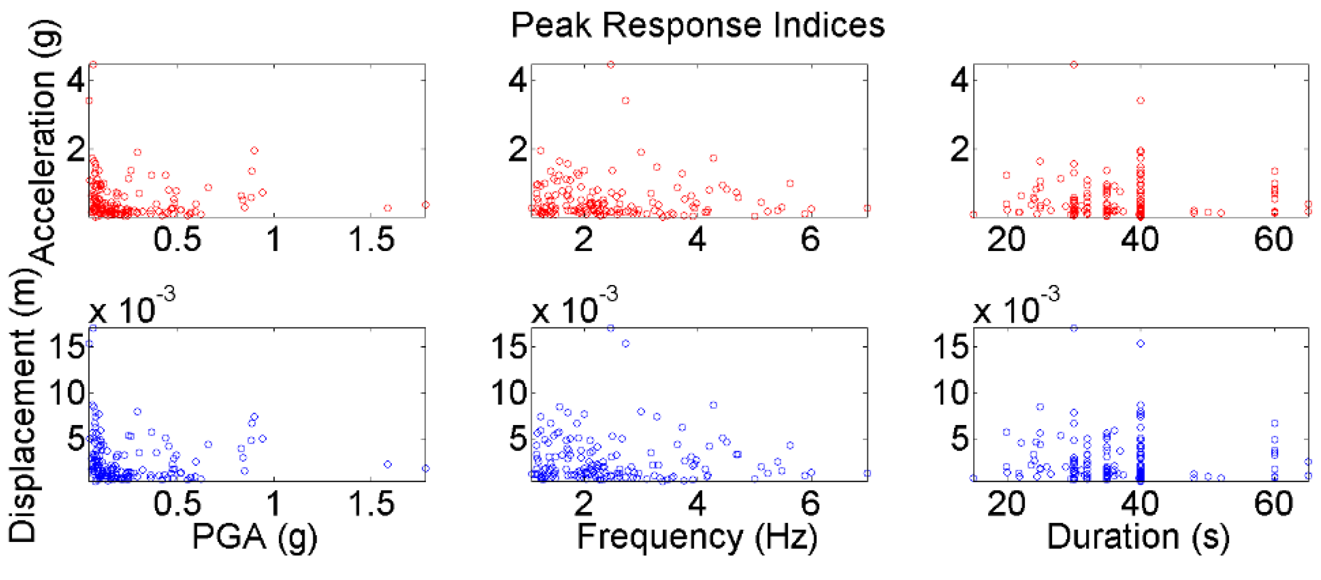
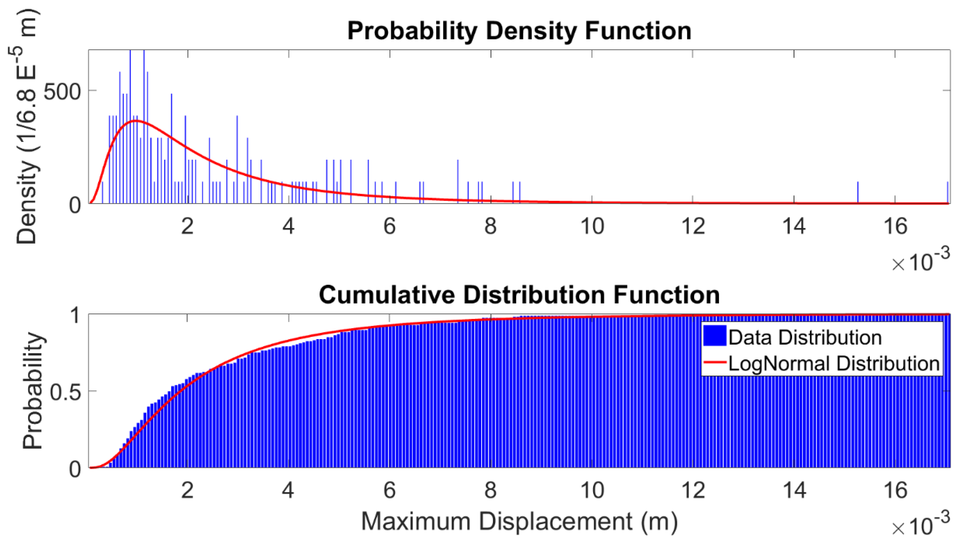
3.2. Simulation of Seismic Response and Reliability

After the optimal modeling parameters are determined and the FEM with limited information is updated, the resultant model can be used as a baseline to predict structural performance under hazardous events. Specifically, in this study, seismic response is scoped, yet similar analysis procedure can be extended to other damaging events. The PEER Strong Motion Database have an extensive set of real earthquake records, therefore, one of these largest sets, 1994 Northridge Earthquake is taken as an exemplary structural demand due to a seismic event [59].

Table 2. Ground motion dataset summary.

Ground Motion Parameter	Range 1	Range 2	Range 3	Range 4
Frequency (Hz)	0–3	3–6	6–10	10–50
Number	112	37	2	0
PGA (g)	$0\text{–}0.1$	0.1–0.4	0.4–1	1–2
Number	50	70	29	2
Duration (s)	0–25	25–50	50–75	75–100
Number	17	120	14	0

shows the overall information about the ground motion dataset features and strong motion parameters.

One hundred and fifty-one earthquake ground motion records are taken from the Northridge Earthquake dataset and used as structural input for time history analyses. With the time history analysis of the baseline model under different earthquake ground motions, the structural response can be probabilistically simulated. Figure 10 shows an example of these analyses illustrating the time and the frequency content of the structural input and outputs.

According to Figure 10, it can be observed that the frequency content of the input ground motion is dominated in low frequencies (below 5 Hz), whereas the structural response peaks around 8–9 Hz. The mode with the lowest frequency, the first mode, is excited more than the second and third modes, and therefore, the response peaks are observed around the first frequency range. This is due to the fact that the higher structural frequencies (e.g., 8.5, 19, 29 Hz) are very far away from relatively low frequency seismic activity. For these reasons, the seismic response is expected to have less structural damage compared with the low frequency civil infrastructure. As a result, the structure behaves in the linear range, yet, it should still be checked whether the bridge maximum deformations exceed certain regulations. One reason is, the nonstructural earthquake damage losses still compose a significant percentage of overall losses [60]. Likewise, even slight damages following a seismic event might result in functionality losses [61]. Besides, it is seen that the low-frequency sensitive displacement response still includes the effects of seismic input, whereas these effects vanish in case of the acceleration response. Finally, and the most important of all, excessive displacements occurring at façade components can lead to glass failure, which possesses safety threat for campus occupants nearby the bridge during the catastrophic incident [62,63].

To summarize the overall dataset results, Figure 11 shows the maximum acceleration and displacement response values indexed according to the strong motion parameters amplitude, frequency, and duration [64], respectively. The analysis results are obtained considering the excitation in the vertical direction. Location of the output corresponds to the absolute maximum displacement value observed on multiple bridge deck nodes throughout the time history analyses.

Time history analysis results are recorded and the maximum response values from each analysis are collected to form a distribution demand. Figure 12 shows the distributed and the cumulative maximum displacement distribution obtained from 151 analysis results. Assuming that the distribution type is log-normal, if the probability density function (PDF) and cumulative distribution function (CDF) are plotted, one can see that the current dataset is a good representative of such type.

The relationship between the arithmetic and logarithmic means can be established with the following relationships,

$${\sigma }_y{}^2=\ln \left(\frac{{\sigma }_x{}^2}{{\mu }_x{}^2}+1\right)$$

$${\mu }_y=\ln \left({\mu }_x\right)-\frac{1}{2}{\sigma }_y{}^2$$

where $\mu$ and $\sigma$ corresponds to mean and standard deviation, whereas y and x subscripts correspond to the normal and lognormal distributions. Distribution obtained from the 151 analysis results is treated as log-normal distribution with the specified mean and standard deviation values, rather than following a fragility curve fitting procedure described in [46,47]. Nevertheless, the red plots show that the log-normal distribution assumption is a good representative of the discrete data distribution obtained from time history analyses. Looking at these CDF values of a particular displacement demand, one can determine the structural reliability under that particular threshold.

After the CDF is determined, the bridge performance can be evaluated according to the reference criteria. An example corresponding to an alter load case is that the US pedestrian steel bridges under live loads are limited by a maximum deflection value of L/1000 [65]. Likewise, allowable live load deflection limit for the bridges in Japan ranges between L/2000 (L shorter than 10 m) and L/500 (L longer than 40 m) depending on the main span length [66]. Considering Mudd-Schapiro Bridge dimensions, L/1000 and L/2000 values correspond to approximately 0.01 and 0.005 m. Static deflection limits for the Ontario highway bridges with pedestrian sidewalks are formulated as a function of the first flexural frequency, and the allowable threshold for 10 Hz is equal to 0.002 m [67]. Although, these parameters are indirectly related to structural damage, extreme relative displacements can possess non-structural threats to the community as well. As mentioned above, Mudd-Schapiro Bridge and its glass facades lay above campus area which has pedestrian access 24 h a day. Quantifying exceedance of certain deflection values is therefore beneficial practice for occupant safety.

Finally, the exceedance probabilities of exemplary reference criteria are investigated according to the CDF values. Considering 0.010, 0.005, and 0.002 m as the performance thresholds, structural reliability values of the data distribution are 0.987, 0.868, and 0.576, respectively. Likewise, log-normal distribution reliability values of the same performance thresholds are within a close range such as 0.981, 0.887, and 0.533, respectively. In general, based on similar reliability values under Northridge Earthquake example, the authorities can take action for pre-event preparation. These can include exemplary decisions such as claiming the structure’s safety, service shutdown, initiating a retrofitting process, destruction if the performance thresholds are unachievable and reconstruction needed. Yet, it should be noted that for a different set of earthquake records with different frequency character, the structural performance is likely to be different. In the future, this issue can be further investigated with ground motion simulation using site-specific spectra (theory-driven), utilize location-aware smartphone seismic networks (measurement-driven), or both. Automated, remote, and computer-aided survey approaches will be more and more important for civil infrastructure systems which is in line with advances in measurement techniques and building information modeling. Basically, imagery data such as point clouds obtained from aerial or terrestrial tools can be converted into FEMs [68,69]. In fact, terrestrial laser scanning is recently linked to FEM updating process, and therefore, SHM [70]. In addition, the advent of drone technologies combined with photogrammetry made it possible to collect aerial information for building inspection [71]. Such complementary tools can also take part in the development of future cyber-physical infrastructure and collocated usage of similar systems is likely to happen in the near future. Nevertheless, in summary, with the multilayered and detailed analysis procedure presented in this paper, response distributions to different datasets can autonomously be performed by a well-structured cyber-physical SHM system.

4. Conclusions

In this study, present and possible future implementations of a crowdsourcing-based mobile cyber-physical SHM system are presented. Civil infrastructure as physical objects are connected to a cyber-structural model and a response simulation scheme, and the real vibration data obtained from smartphone users are used to calibrate these model parameters. This procedure includes a number of information processing phases such as mobile, server, and administrative components. The mobile platform digitizes structural vibrations via accelerometers and submits it to the server. The server conducts modal identification, returns, and stores the analysis results. The identification results obtained from smartphone sensors are used to update the FEM and increase its accuracy by minimizing the error between the model and the identified modal parameters, which is formerly created with limited information and modeling uncertainties.

Using the updated model as a baseline, structural responses subjected to 151 earthquake records are simulated by time history analyses. The displacement demand distribution obtained from the time history analysis results is evaluated according to the exemplary maximum allowed deflection criteria. Finally, for an earthquake scenario with a wide set of records, one can determine the structural reliability according to the desired performance levels. This information can provide the decision makers with a good foundation for risk assessment, preparedness, and mitigation. Based on the evaluation results of this cyber-physical information flow, the bridge service can be interrupted, structural members can be retrofitted, or the existing structure can be demolished if there is no feasible maintenance scenario. As the volume of invisible operations in computational zone increases, the cyber loops will become more remote and automated.

The framework is demonstrated on an actual pedestrian bridge structure, and the results are presented. The results show that even with limited information, accurate FEMs can be developed with the help of a model updating procedure. Besides, the necessary information is provided by smartphone sensor data and crowdsourcing which solely relies on participatory sensing and pure citizen contribution. Once the physical information is extracted from the sensors, the corresponding data can be combined with a deep mathematical process without any human intervention. Automation, connectivity, scalability, and mobility of the presented platform has a great potential for future mobile cyber-physical SHM systems. Especially, as the seismic monitoring arrays become dense and abundant (e.g., smartphone seismometers), seismic performance of a structure can be simultaneously evaluated with ubiquitous data according to the reference code regulations and standards.

References

1. ASCE. Seismic Evaluation and Retrofit of Existing Buildings (ASCE/SEI 41-13); American Society of Civil Engineers: Reston, VA, USA, 2014. [Google Scholar]
2. AASHTO. LRFD Bridge Design Specifications; American Association of State Highway and Transportation Officials: Washington, DC, USA, 2015. [Google Scholar]
3. Doebling, S.W.; Farrar, C.R.; Prime, M.B. A summary review of vibration-based damage identification methods. Shock Vib. Dig. 1998, 30, 91–105. [Google Scholar] [CrossRef]
4. Carden, E.P.; Fanning, P. Vibration based condition monitoring: A review. Struct. Health Monit. 2004, 3, 355–377. [Google Scholar] [CrossRef]
5. Brownjohn, J.M. Structural health monitoring of civil infrastructure. Philos. Trans. R. Soc. Lond. A Math. Phys. Eng. Sci. 2007, 365, 589–622. [Google Scholar] [CrossRef] [PubMed]
6. Farrar, C.R.; Worden, K. An introduction to structural health monitoring. Philos. Trans. R. Soc. Lond. A Math. Phys. Eng. Sci. 2007, 365, 303–315. [Google Scholar] [CrossRef] [PubMed]
7. Wahbeh, A.M.; Caffrey, J.P.; Masri, S.F. A vision-based approach for the direct measurement of displacements in vibrating systems. Smart Mater. Struct. 2003, 12, 785. [Google Scholar] [CrossRef]
8. Lee, J.J.; Shinozuka, M. A vision-based system for remote sensing of bridge displacement. Ndt E Int. 2006, 39, 425–431. [Google Scholar] [CrossRef]
9. Feng, D.; Feng, M.Q.; Ozer, E.; Fukuda, Y. A vision-based sensor for noncontact structural displacement measurement. Sensors 2015, 15, 16557–16575. [Google Scholar] [CrossRef]
10. Farrar, C.R.; Park, G.; Allen, D.W.; Todd, M.D. Sensor network paradigms for structural health monitoring. Struct. Control Health Monit. 2006, 13, 210–225. [Google Scholar] [CrossRef]
11. Lynch, J.P.; Loh, K.J. A summary review of wireless sensors and sensor networks for structural health monitoring. Shock Vib. Dig. 2006, 38, 91–130. [Google Scholar] [CrossRef]
12. Gao, Y.; Spencer, B.F.; Ruiz-Sandoval, M. Distributed Computing Strategy for Structural Health Monitoring. Struct. Control Health Monit. 2006, 13, 488–507. [Google Scholar] [CrossRef]
13. Lynch, J.P. An overview of wireless structural health monitoring for civil structures. Philos. Trans. R. Soc. Lond. A Math. Phys. Eng. Sci. 2007, 365, 345–372. [Google Scholar] [CrossRef] [PubMed]
14. Aygün, B.; Cagri Gungor, V. Wireless sensor networks for structure health monitoring: Recent advances and future research directions. Sens. Rev. 2011, 31, 261–276. [Google Scholar] [CrossRef]
15. Prasad, P. Recent trend in wireless sensor network and its applications: A survey. Sens. Rev. 2015, 35, 229–236. [Google Scholar] [CrossRef]
16. Farhey, D.N. Integrated virtual instrumentation and wireless monitoring for infrastructure diagnostics. Struct. Health Monit. 2006, 5, 29–43. [Google Scholar] [CrossRef]
17. Liu, S.C.; Tomizuka, M.; Ulsoy, G. Strategic issues in sensors and smart structures. Struct. Control Health Monit. 2006, 13, 946–957. [Google Scholar] [CrossRef]
18. Spencer, B.F.; Ruiz-Sandoval, M.E.; Kurata, N. Smart sensing technology: Opportunities and challenges. Struct. Control Health Monit. 2004, 11, 349–368. [Google Scholar] [CrossRef]
19. Jeong, M.J.; Koh, B.H. A decentralized approach to damage localization through smart wireless sensors. Smart Struct. Syst. 2009, 5, 43–54. [Google Scholar] [CrossRef]
20. Taylor, S.G.; Farinholt, K.M.; Flynn, E.B.; Figueiredo, E.; Mascarenas, D.L.; Moro, E.A.; Park, G.; Todd, M.D.; Farrar, C.R. A mobile-agent-based wireless sensing network for structural monitoring applications. Meas. Sci. Technol. 2009, 20, 045201. [Google Scholar] [CrossRef]
21. Chen, B.; Liu, W. Mobile agent computing paradigm for building a flexible structural health monitoring sensor network. Comput.-Aided Civ. Infrastruct. Eng. 2010, 25, 504–516. [Google Scholar] [CrossRef]
22. Zhu, D.; Yi, X.; Wang, Y.; Lee, K.M.; Guo, J. A mobile sensing system for structural health monitoring: Design and validation. Smart Mater. Struct. 2010, 19, 055011. [Google Scholar] [CrossRef]
23. OBrien, E.J.; Keenahan, J. Drive-by damage detection in bridges using the apparent profile. Struct. Control Health Monit. 2015, 22, 813–825. [Google Scholar] [CrossRef]
24. Sun, H.; Büyüköztürk, O. Identification of traffic-induced nodal excitations of truss bridges through heterogeneous data fusion. Smart Mater. Struct. 2015, 24, 075032. [Google Scholar] [CrossRef]
25. Lienhart, W. Challenges in the analysis of inhomogeneous structural monitoring data. J. Civ. Struct. Health Monit. 2013, 3, 247–255. [Google Scholar] [CrossRef]
26. Chatzi, E.N.; Smyth, A.W. The unscented Kalman filter and particle filter methods for nonlinear structural system identification with non-collocated heterogeneous sensing. Struct. Control Health Monit. 2009, 16, 99–123. [Google Scholar] [CrossRef]
27. Cho, S.; Giles, R.K.; Spencer, B.F. System identification of a historic swing truss bridge using a wireless sensor network employing orientation correction. Struct. Control Health Monit. 2015, 22, 255–272. [Google Scholar] [CrossRef]
28. Morgenthal, G.; Höpfner, H. The application of smartphones to measuring transient structural displacements. J. Civ. Struct. Health Monit. 2012, 2, 149–161. [Google Scholar] [CrossRef]
29. Oraczewski, T.; Staszewski, W.J.; Uhl, T. Nonlinear acoustics for structural health monitoring using mobile, wireless and smartphone-based transducer platform. J. Intell. Mater. Syst. Struct. 2015. [Google Scholar] [CrossRef]
30. Zhao, X.; Han, R.; Ding, Y.; Yu, Y.; Guan, Q.; Hu, W.; Ou, J. Portable and convenient cable force measurement using smartphone. J. Civ. Struct. Health Monit. 2015, 5, 481–491. [Google Scholar] [CrossRef]
31. Feng, M.; Fukuda, Y.; Mizuta, M.; Ozer, E. Citizen Sensors for SHM: Use of Accelerometer Data from Smartphones. Sensors 2015, 15, 2980–2998. [Google Scholar] [CrossRef] [Green Version]
32. Ozer, E.; Feng, M.Q.; Feng, D. Citizen Sensors for SHM: Towards a Crowdsourcing Platform. Sensors 2015, 15, 14591–14614. [Google Scholar] [CrossRef]
33. Ozer, E.; Feng, M.Q. Synthesizing spatiotemporally sparse smartphone sensor data for bridge modal identification. Smart Mater. Struct. 2016, 25, 085007. [Google Scholar] [CrossRef]
34. Ozer, E.; Feng, M.Q. Direction-sensitive smart monitoring of structures using heterogeneous smartphone sensor data and coordinate system transformation. Smart Mater. Struct. 2017, 26, 045026. [Google Scholar] [CrossRef]
35. Lasi, H.; Fettke, P.; Kemper, H.G.; Feld, T.; Hoffmann, M. Industry 4.0. Bus. Inf. Syst. Eng. 2014, 6, 239. [Google Scholar] [CrossRef]
36. Lee, J.; Bagheri, B.; Kao, H.A. A cyber-physical systems architecture for industry 4.0-based manufacturing systems. Manuf. Lett. 2015, 3, 18–23. [Google Scholar] [CrossRef]
37. Lee, E.A. The past, present and future of cyber-physical systems: A focus on models. Sensors 2015, 15, 4837–4869. [Google Scholar] [CrossRef] [PubMed]
38. Schirner, G.; Erdogmus, D.; Chowdhury, K.; Padir, T. The future of human-in-the-loop cyber-physical systems. Computer 2013, 46, 36–45. [Google Scholar] [CrossRef]
39. Wu, F.J.; Kao, Y.F.; Tseng, Y.C. From wireless sensor networks towards cyber physical systems. Pervasive Mob. Comput. 2011, 7, 397–413. [Google Scholar] [CrossRef]
40. Kim, K.D.; Kumar, P.R. Cyber–physical systems: A perspective at the centennial. Proc. IEEE 2012, 100, 1287–1308. [Google Scholar]
41. Hu, X.; Chu, T.; Chan, H.; Leung, V. Vita: A crowdsensing-oriented mobile cyber-physical system. Emerg. Top. Comput. IEEE Trans. 2013, 1, 148–165. [Google Scholar] [CrossRef]
42. Atzori, L.; Iera, A.; Morabito, G. The internet of things: A survey. Comput. Netw. 2010, 54, 2787–2805. [Google Scholar] [CrossRef]
43. Gubbi, J.; Buyya, R.; Marusic, S.; Palaniswami, M. Internet of Things (IoT): A vision, architectural elements, and future directions. Future Gener. Comput. Syst. 2013, 29, 1645–1660. [Google Scholar] [CrossRef] [Green Version]
44. Gershenfeld, N.; Krikorian, R.; Cohen, D. The Internet of things. Sci. Am. 2004, 291, 76. [Google Scholar] [CrossRef]
45. Miorandi, D.; Sicari, S.; De Pellegrini, F.; Chlamtac, I. Internet of things: Vision, applications and research challenges. Ad Hoc Netw. 2012, 10, 1497–1516. [Google Scholar] [CrossRef] [Green Version]
46. Özer, E.; Soyöz, S. Vibration-based damage detection and seismic performance assessment of bridges. Earthq. Spectra 2015, 31, 137–157. [Google Scholar] [CrossRef]
47. Ozer, E.; Feng, M.Q.; Soyoz, S. SHM-integrated bridge reliability estimation using multivariate stochastic processes. Earthq. Eng. Struct. Dyn. 2015, 44, 601–618. [Google Scholar] [CrossRef]
48. Ozer, E. Multisensory Smartphone Applications in Vibration-Based Structural Health Monitoring. Ph.D. Thesis, Columbia University, New York, NY, USA, 2016. [Google Scholar]
49. McKenna, F. OpenSees: A framework for earthquake engineering simulation. Comput. Sci. Eng. 2011, 13, 58–66. [Google Scholar] [CrossRef]
50. Ozer, E.; Feng, M.Q. Biomechanically influenced mobile and participatory pedestrian data for bridge monitoring. Int. J. Distrib. Sens. Netw. 2017, 13, 1550147717705240. [Google Scholar] [CrossRef]
51. Suh, S.C.; Tanik, U.J.; Carbone, J.N.; Eroglu, A. Applied Cyber-Physical Systems; Springer: New York, NY, USA, 2014. [Google Scholar]
52. Liu, C.H.; Zhang, Y. Cyber Physical Systems: Architectures, Protocols and Applications; CRC Press: Boca Raton, FL, USA, 2015. [Google Scholar]
53. Hu, F. Cyber-Physical Systems: Integrated Computing and Engineering Design; CRC Press: Boca Raton, FL, USA, 2013. [Google Scholar]
54. Siddesh, G.M.; Deka, G.; Srinivasa, K.G.; Patnaik, L.M. Cyber-Physical Systems: A Computational Perspective; CRC Press: Boca Raton, FL, USA, 2016. [Google Scholar]
55. Ghanem, R.; Shinozuka, M. Structural-system identification. I: Theory. J. Eng. Mech. 1995, 121, 255–264. [Google Scholar] [CrossRef]
56. Shinozuka, M.; Ghanem, R. Structural system identification. II: Experimental verification. J. Eng. Mech. 1995, 121, 265–273. [Google Scholar] [CrossRef]
57. Dashti, S.; Bray, J.D.; Reilly, J.; Glaser, S.; Bayen, A.; Mari, E. Evaluating the reliability of phones as seismic monitoring instruments. Earthq. Spectra 2014, 30, 721–742. [Google Scholar] [CrossRef]
58. Shinozuka, M.; Deodatis, G. Simulation of stochastic processes by spectral representation. Appl. Mech. Rev. 1991, 44, 191–204. [Google Scholar] [CrossRef]
59. Chiou, B.; Darragh, R.; Gregor, N.; Silva, W. NGA project strong-motion database. Earthq. Spectra 2008, 24, 23–44. [Google Scholar] [CrossRef]
60. Kircher, C.A.; Reitherman, R.K.; Whitman, R.V.; Arnold, C. Estimation of earthquake losses to buildings. Earthq. Spectra 1997, 13, 703–720. [Google Scholar] [CrossRef]
61. Nielson, B.G.; DesRoches, R. Analytical seismic fragility curves for typical bridges in the central and southeastern United States. Earthq. Spectra 2007, 23, 615–633. [Google Scholar] [CrossRef]
62. GANA, B. GANA Glazing Manual; Glass Association of North America: Topeka, KS, USA, 2004. [Google Scholar]
63. O’Brien, W.C., Jr.; Memari, A.M.; Kremer, P.A.; Behr, R.A. Fragility curves for architectural glass in stick-built glazing systems. Earthq. Spectra 2012, 28, 639–665. [Google Scholar] [CrossRef]
64. Kramer, S.L. Geotechnical Earthquake Engineering; Prentice Hall: Upper Saddle River, NJ, USA, 1996. [Google Scholar]
65. Roeder, C.W.; Barth, K.E.; Bergman, A. Effect of live-load deflections on steel bridge performance. J. Bridge Eng. 2004, 9, 259–267. [Google Scholar] [CrossRef]
66. Nishikawa, K.; Murakoshi, J.; Matsuki, T. Study on the fatigue of steel highway bridges in Japan. Constr. Build. Mater. 1998, 12, 133–141. [Google Scholar] [CrossRef]
67. Billing, J.R. Dynamic loading and testing of bridges in Ontario. Can. J. Civ. Eng. 1984, 11, 833–843. [Google Scholar] [CrossRef]
68. Hinks, T.; Carr, H.; Truong-Hong, L.; Laefer, D.F. Point cloud data conversion into solid models via point-based voxelization. J. Surv. Eng. 2012, 139, 72–83. [Google Scholar] [CrossRef]
69. Castellazzi, G.; D’Altri, A.; Bitelli, G.; Selvaggi, I.; Lambertini, A. From laser scanning to finite element analysis of complex buildings by using a semi-automatic procedure. Sensors 2015, 15, 18360–18380. [Google Scholar] [CrossRef]
70. Yang, H.; Xu, X.; Neumann, I. Laser scanning-based updating of a finite-element model for structural health monitoring. IEEE Sens. J. 2015, 16, 2100–2104. [Google Scholar] [CrossRef]
71. Rakha, T.; Gorodetsky, A. Review of Unmanned Aerial System (UAS) applications in the built environment: Towards automated building inspection procedures using drones. Autom. Constr. 2018, 93, 252–264. [Google Scholar] [CrossRef]
Figure 1. Cyber-physical processes of CS4SHM system.
Applsci 09 02840 g001
Figure 2. Mudd Schapiro Link Bridge.
Applsci 09 02840 g002
Figure 3. Conceptual CPS scheme for smartphone-based SHM.
Applsci 09 02840 g003
Figure 4. Exemplary crowdsourced submission time histories and Fourier spectra.
Applsci 09 02840 g004
Figure 5. Finite element model nodes, elements and axes.
Applsci 09 02840 g005
Figure 6. Finite element modeling uncertainties.
Applsci 09 02840 g006
Figure 7. Integration scheme of Matlab and OpenSees software.
Applsci 09 02840 g007
Figure 8. Modal frequency error surfaces for fixed-fixed, fixed-pinned, fixed-roller BCs.
Applsci 09 02840 g008
Figure 9. Updated FEM modal parameters for fixed-fixed, fixed-pinned, fixed-roller BCs.
Applsci 09 02840 g009
Figure 10. Exemplary input ground motion and simulated structural response.
Applsci 09 02840 g010
Figure 11. Peak responses indexed according to the strong motion parameters.
Applsci 09 02840 g011
Figure 12. Maximum displacement demands based on Northridge Earthquake records.
Applsci 09 02840 g012