Article

Detection of a Semi-Rough Target in Turbulent Atmosphere by an Electromagnetic Gaussian Schell-Model Beam

1
Shandong Provincial Engineering and Technical Center of Light Manipulations & Shandong Provincial Key Laboratory of Optics and Photonic Device, School of Physics and Electronics, Shandong Normal University, Jinan 250014, China
2
School of Physical Science and Technology, Soochow University, Suzhou 215006, China
*
Authors to whom correspondence should be addressed.
Appl. Sci. 2019, 9(14), 2790; https://doi.org/10.3390/app9142790
Submission received: 19 April 2019 / Revised: 3 July 2019 / Accepted: 9 July 2019 / Published: 11 July 2019
(This article belongs to the Special Issue Recent Advances in Statistical Optics and Plasmonics)

Abstract

:
The interaction of an electromagnetic Gaussian Schell-model beam with a semi-rough target located in atmospheric turbulence was studied by means of a tensor method, and the corresponding inverse problem was analyzed. The equivalent model was set up on the basis of a bistatic laser radar system and a rough target located in a turbulent atmosphere. Through mathematical deduction, we obtained detailed information about the parameters of the semi-rough target by measuring the beam radius, coherence radius of the incident beam and the polarization properties of the returned beam.

1. Introduction

The issue of laser beam propagation in atmospheric turbulence has been explored widely over the past decades. It is well-known that atmospheric turbulence induces random variations in the phase, propagating direction and intensity of beams, which are characterized by beam spreading, beam wander and scintillation [1,2,3]. These phenomena have negative effects on the laser transport performance. In contrast to fully coherent beams, partially coherent beams are better at resisting the negative effects induced by atmospheric turbulence, and this has been verified in several experiments [4,5]. Thus, partially coherent beams are expected to improve the performance of laser communication systems [6,7]. The Gaussian Schell-model (GSM) beam [8,9] is a representative partially coherent beam, whose intensity and spectral degree of coherence satisfy Gaussian distributions, and much attention has been paid to its transmission properties in free space or random media. Several relevant research methods have been proposed [10,11,12].
Although researchers have made many efforts on the subject of GSM beam propagation through atmospheric turbulence [13,14,15,16,17], most studies have been limited to scalar fields without considering the vector properties of light. The degree of polarization represents the relevance of two rectangular components of the electric field at one single point [18,19,20]. In 2003, a unified theory of coherence and polarization was proposed [21], and this is highly advantageous for in-depth study of the spectrum, coherence and polarization of the beam [22,23,24]. The electromagnetic Gaussian Schell-model (EGSM) beam is a classical partially coherent vector beam and any point in this field has the same polarization [25,26,27,28,29,30]. In recent years, a number of researchers have increasingly focused on the propagation of EGSM beams in free space and in random media [31,32,33,34,35,36,37,38]. In comparison with the GSM beam, under appropriate conditions, the EGSM beam can significantly reduce the light fluctuations caused by atmospheric turbulence, and this conclusion has been well verified [39,40,41]. There are numerous studies on the effect of atmospheric turbulence on the coherence degree and polarization state of an EGSM beam [42,43,44,45,46]. Many experimental and theoretical studies have demonstrated that EGSM beams have significant applications in many areas such as free-space optical communications, remote sensing, LIDAR systems, and optical illumination [47,48,49].
In an active bistatic LIDAR system, the returned beam passing through atmospheric turbulence aggravates the system noise, and then, the detection accuracy and efficiency is reduced. Many studies have found that the properties of laser beams are affected by the transmission medium, besides target scattering [50,51,52,53,54]. Accordingly, it is necessary to study the combined action of the atmospheric turbulence and target scattering on laser beams with the object embedded in atmospheric turbulence. In previous work, attention has been focused on the forward transmission in atmospheric turbulence. The interaction of the EGSM beam with a semi-rough target located in atmospheric turbulence was explored in [39]; the paper qualitatively analyzed the combined effect of the surface roughness and the object size on the coherence and polarization. In this paper, through inversion analysis of the interaction of isotropic EGSM beams with a semi-rough target in atmospheric turbulence, we found that it is possible to quantitatively obtain accurate parameters of the object surface by contrasting the characteristics of the incident beam and its returned beam.
We assumed the atmospheric turbulence to be homogeneous and isotropic. Moreover, the surface of the target was set as semi-rough and isotropic. The model of the target consisted of two components: a thin lens with good reflective properties and a thin phase screen to cause phase perturbations [55,56,57,58]. The complete process was divided into three main stages. Firstly, the EGSM beam travels from the source plane to the target plane in atmospheric turbulence. Then, after the interaction of the laser beam with the object surface, the beam propagates from the target plane to the receiver plane. Finally, we calculated the degree of polarization of the returned beam and the detailed parameters of the object were derived.

2. Theoretical Analysis

We analyzed the propagation process with the help of a tensor method. The tensor method developed in [59] is quite useful for treating the propagation of a partially coherent beam in random media directly. With the aid of the calculation method, the atmospheric turbulence and the object surface are embedded in the optical system. The object is supposed to be isotropic. The representative model of the object is composed of a Gaussian mirror and a thin phase screen as shown in Figure 1 [56,57]. All the optical elements in the system can be expressed in 4 × 4 tensor form.
According to the unified theory of coherence and polarization, 2 × 2 cross-spectral density matrices are used to describe the second-order statistical properties of the EGSM beam. In this paper, we use vector symbols to denote the matrices in different parts. W i j ( r ˜ ) represents the EGSM beam generated by the source, W i j ( t ˜ ) represents the beam at the target plane, and W i j ( ρ ˜ ) represents the beam at the receiver plane.

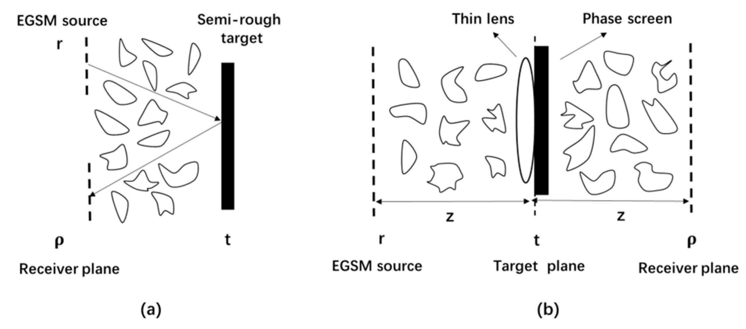
2.1. Transmission from the Source to the Target Plane

At z = 0, the general expression for the elements of the cross-spectral density (CSD) matrix of the isotropic EGSM beam in the space-frequency domain can be expressed as follows [4]:
W i j ( r 1 , r 2 ) = E i ( r 1 ) E j ( r 2 ) = A i A j B i j exp [ r 1 2 4 σ i 2 r 2 2 4 σ j 2 ] exp [ ( r 2 r 1 ) 2 2 δ i j 2 ] , ( i = x , y ; j = x , y ) .
In this model, A i , A j are the spectral amplitudes of the electric field components; B i j is the complex correlation coefficient between two electric field components; σ i , σ j are the beam radius along two orthogonal directions, respectively; δ i j denotes the transverse coherence radius of field components, respectively. Also, δ i j = δ j i , B i j = B j i follow from the fact W i j ( r 1 , r 2 , ω ) = W j i ( r 2 , r 1 , ω ) , which is obtained from the definition of the correlation matrix W. For a uniformly polarized source, we set σ x = σ y = σ [60]. Under this condition, every point in the source plane has an identical degree of polarization. Finally, the constraints to ensure the source can be realized are obtained as follows [21]:
δ x x 2 + δ y y 2 2 δ x y δ x x δ y y | B x y | ,
1 4 σ 2 + 1 δ i i 2 2 π 2 λ 2 ( i = x , y ) .
The factor B i j obeys the following properties [40]:
B i j = 1   when i = j ;   | B i j | 1   when   i j
In the source plane, the elements of the CSD matrix of the beam generated by an EGSM source can be expressed in the following form [17]
W i j ( r ˜ ) = A i A j B i j exp [ i k 2 r ˜ T M 0 i j 1 r ˜ ] , ( i = x , y ; j = x , y ) ,
M 0 i j 1 = ( ( i 2 k σ 2 i k δ i j 2 ) I i k δ i j 2 I i k δ i j 2 I ( i 2 k σ 2 i k δ i j 2 ) I ) ,
where r ˜ T = ( r 1 , r 2 ) T , I is a 2 × 2 unit matrix and M 0 i j 1 is a transpose symmetric matrix in the source plane. Following [54], the atmospheric turbulence is supposed to be homogeneous and isotropic. The transmission process of the beam can be expressed in the tensor form. From the source plane to the target plane, under the paraxial approximation, the atmospheric propagation obeys the following generalized Collins formula [52],
W i j ( t ˜ ) = k 2 4 π det ( B ˜ ) 1 2 W i j ( r ˜ ) exp [ i k 2 ( r ˜ T B ˜ 1 A ˜ r ˜ r ˜ T B ˜ 1 t ˜ t ˜ T B ˜ 1 r ˜ + t ˜ T D ˜ B ˜ 1 t ˜ ) ] × exp [ i k 2 ( r ˜ T P ˜ r ˜ + r ˜ T P ˜ t ˜ + t ˜ T P ˜ t ˜ ) ] d r ˜ .
Substituting from Equations (5)–(7), we obtain the following expression for the elements of the CSD matrix of the EGSM beam at the target plane.
W i j ( t ˜ ) = A i A j B i j [ det ( A ˜ + B ˜ M 0 i j 1 + B ˜ P ˜ ) ] 1 2 exp [ i k 2 t ˜ T M 1 i j 1 t ˜ ] ,
M 1 i j 1 = ( B ˜ 1 1 2 P ˜ ) T ( M 0 1 + B ˜ 1 A ˜ + P ˜ ) 1 ( B ˜ 1 1 2 P ˜ ) + ( D ˜ B ˜ 1 + P ˜ ) .
In the derivation process of Equation (8), the integral formula exp ( a x 2 ) d x = π a has been used. Here, M 1 i j 1 denotes the partially coherent complex curvature tensors in the target plane, A ˜ , B ˜ , D ˜ and P ˜ are all 4 × 4 transfer matrices that describe the optical system,
A ˜ = ( I 0 I 0 I I ) , B ˜ = ( z I 0 I 0 I z I ) , D ˜ = ( ( 1 z / f ) I 0 I 0 I ( 1 z / f ) I ) , P ˜ = 2 i k ρ 0 2 ( I I I I ) ,
ρ 0 = ( 0.545 k 2 C n 2 z ) 3 / 5 ,
where C n 2 is the refractive-index structure parameter and k = 2 π / λ is the wave number. ρ 0 is the coherence length of a spherical length propagating in weak atmospheric turbulence with Kolmogorov power spectrum.

2.2. Transmission from the Target to the Receiver Plane

As mentioned in the previous section, we assume that the surface of the target is isotropic and semi-rough. We describe the surface using a helpful model proposed by Goodman several years ago [58]. The model can be thought of so that, under some conditions, surface scattering is regarded as passing through a thin random phase screen. Therefore, we use Equations (12) and (13) to describe the action of the target scattering on laser beams.
T ( t 1 ) T ( t 2 ) = 4 π β 2 k 2 exp [ i k 2 t ˜ T T ˜ t ˜ ] ,
T ˜ = ( ( 2 i k w R 2 2 i k l c 2 ) I 2 i k l c 2 I 2 i k l c 2 I ( 2 i k w R 2 2 i k l c 2 ) I ) ,
where “< >” denotes an ensemble average, “∗” denotes the complex conjugate, and t ˜ T = ( t 1 , t 2 ) T . w R is the target size, l c is the typical transverse correlation width, and β is the normalization parameter.
Similar to Equation (7), after the combined action of atmospheric turbulence and target scattering on a laser beam, the atmospheric propagation obeys the following generalized Collins formula from the target plane to the receiver plane [52].
W i j ( ρ ˜ ) = k 2 4 π det ( B ˜ ) 1 2 W i j ( t ˜ ) × T ( t 1 ) T ( t 2 ) × exp [ i k 2 ( t ˜ T B ˜ 1 t ˜ t ˜ T B ˜ 1 ρ ˜ ρ ˜ T B ˜ 1 t ˜ + ρ ˜ T B ˜ 1 ρ ˜ ) ] × exp [ i k 2 ( t ˜ T P ˜ t ˜ + t ˜ T P ˜ ρ ˜ + ρ ˜ T P ˜ ρ ˜ ) ] d t ˜ .
Substituting from Equations (8), (12)–(14), the elements of the CSD matrix of the EGSM beam at the receiver plane are given by the following expressions,
W i j ( ρ ˜ ) = 4 π β 2 A i A j B i j k 2 [ d e t ( I ˜ + B ˜ M 1 i j 1 + B ˜ T ˜ + B ˜ P ˜ ) ] 1 2 [ d e t ( A ˜ + B ˜ M 0 i j 1 + B ˜ P ˜ ) ] 1 2 exp [ i k 2 ρ ˜ T M 2 i j 1 ρ ˜ ] ,
M 2 i j 1 = P ˜ + B ˜ 1 ( B ˜ 1 1 2 P ˜ ) T ( M 1 i j 1 + T ˜ + B ˜ 1 + P ˜ ) 1 ( B ˜ 1 1 2 P ˜ ) .
where M 2 ij 1 denote the partially coherent complex curvature tensor in the receiver plane, respectively. According to the tensor method, we can express M 2 ij 1 as follows,
W i j ( ρ 1 , ρ 2 ) = 4 π β 2 A i A j B i j k 2 [ det ( I ˜ + B ˜ M 1 i j 1 + B ˜ T ˜ + B ˜ P ˜ ) ] 1 2 [ det ( A ˜ + B ˜ M 0 i j 1 + B ˜ P ˜ ) ] 1 2 × exp [ ρ 1 2 + ρ 2 2 4 σ i j o u t 2 ] × exp [ ( ρ 2 ρ 1 ) 2 2 δ i j o u t 2 ] × exp [ i k ( ρ 1 2 ρ 2 2 ) 2 R i j o u t ] .
Then, Equation (15) reduces to
M 2 i j 1 = ( m 21 I m 22 I m 23 I m 24 I ) = ( R i j o u t 1 + ( i 2 k σ i j o u t 2 i k δ i j o u t 2 ) I i k δ i j o u t 2 I i k δ i j o u t 2 I R i j o u t 1 + ( i 2 k σ i j o u t 2 i k δ i j o u t 2 ) I ) .
From Equation (18), we can obtain the following equations
1 σ i j out 2 = k i ( m 21 + m 24 ) 2 k i m 22 .
By substituting Equations (6), (9), (13), (16), (18) and (19), we obtain the following equations
1 σ i j o u t 2 = e 2 i j l c 2 w R 2 + f 2 i j l c 2 w R 4 a 1 i j w R 4 + 2 b 1 i j w R 2 + b 1 i j l c 2 + c 1 i j l c 2 w R 2 + d 1 i j l c 2 w R 4 ,
a 1 i j = 8 R 1 i j 2 z 2 ρ 0 2 δ 1 i j 2 σ 1 i j 2 ,
b 1 i j = 16 R 1 i j 2 z 2 ρ 0 2 δ 1 i j 2 σ 1 i j 4 ,
c 1 i j = R 1 i j 2 z 2 σ 1 i j 2 [ 16 ρ 0 2 σ 1 i j 2 + δ 1 i j 2 ( 8 ρ 0 2 + 32 σ 1 i j 2 ) ] ,
d 1 i j = 8 k 2 R 1 i j z ρ 0 2 δ 1 i j 2 σ 1 i j 4 + 4 k 2 z 2 ρ 0 2 δ 1 i j 2 σ 1 i j 4 + R 1 i j 2 [ 4 k 2 ρ 0 2 δ 1 i j 2 σ 1 i j 4 + z 2 ( 4 ρ 0 2 σ 1 i j 2 + δ 1 i j 2 ( ρ 0 2 + 8 σ 1 i j 2 ) ) ] ,
e 2 i j = 16 R 1 i j 2 k 2 ρ 0 2 δ 1 i j 2 σ 1 i j 4 ,
f 2 i j = 4 R 1 i j 2 k 2 ρ 0 2 δ 1 i j 2 σ 1 i j 2 ,
δ 1 i j 2 = 4 k 2 ρ 0 4 δ i j 2 σ 4 + z 2 ρ 0 2 ( 4 ρ 0 2 σ 2 + δ i j 2 ( ρ 0 2 + 8 σ 2 ) ) k 2 ρ 0 2 ( 24 δ i j 2 + 4 ρ 0 2 ) σ 4 + z 2 ( 8 ρ 0 2 σ 2 + δ i j 2 ( 2 ρ 0 2 + 12 σ 2 ) ) ,
σ 1 i j 2 = 4 k 2 ρ 0 2 δ i j 2 σ 4 + z 2 ( 4 ρ 0 2 σ 2 + δ i j 2 ( ρ 0 2 + 8 σ 2 ) ) 4 k 2 ρ 0 2 δ i j 2 σ 2 ,
R 1 i j 1 = 1 f + z ( ρ 0 2 σ 2 + δ ij 2 ( 0.25 ρ 0 2 + 3 σ 2 ) ) k 2 ρ 0 2 δ i j 2 σ 4 + z 2 ( ρ 0 2 σ 2 + δ i j 2 ( 0.25 ρ 0 2 + 2 σ 2 ) ) .

2.3. Degree of the Polarization

According to the definition, the spectral degree of polarization of the EGSM beam at a point ρ is defined as the following expression [18],
P = 1 4 det W i j ( ρ , ρ ) T r W i j ( ρ , ρ ) 2 = ( F x x exp ( ρ 2 2 1 σ x x o u t 2 ) F y y exp ( ρ 2 2 1 σ y y o u t 2 ) ) 2 + 4 F x y F y x exp ( ρ 2 2 ( 1 σ x y o u t 2 + 1 σ y x o u t 2 ) ) | F x x exp ( ρ 2 2 1 σ x x o u t 2 ) + F y y exp ( ρ 2 2 1 σ y y o u t 2 ) | ,
F i j = 4 π β 2 B i j A i A j k 2 [ d e t ( I ˜ + B ˜ M 1 i j 1 + B ˜ T ˜ + B ˜ P ˜ ) ] 1 2 [ d e t ( A ˜ + B ˜ M 0 i j 1 + B ˜ P ˜ ) ] 1 2 , ( i = x , y ; j = x , y )
where “Tr” and “det” denote the trace and the determinant of a matrix.
The amplitudes of the electric field components along x and y directions are selected with the same value, then, in Equation (4) A x = A y = 1 and δ x x = δ y y = δ . Using the relation, δ x y = δ y x and Equations (4), (9), (16) and (30), we can obtain the degree of polarization of the received beam
P o u t = | B x y | [ d e t ( I ˜ + B ˜ M 1 x x 1 + B ˜ T ˜ + B ˜ P ˜ ) ] 1 2 [ d e t ( A ˜ + B ˜ M 0 x x 1 + B ˜ P ˜ ) ] 1 2 [ d e t ( I ˜ + B ˜ M 1 x y 1 + B ˜ T ˜ + B ˜ P ˜ ) ] 1 2 [ d e t ( A ˜ + B ˜ M 0 x y 1 + B ˜ P ˜ ) ] 1 2 exp ( ρ 2 2 ( 1 σ x y o u t 2 1 σ x x o u t 2 ) ) .
For simplicity, we choose points on the optical axis ( ρ = 0 ), then Equation (32) reduces to the following form
P o u t = | B x y | [ d e t ( I ˜ + B ˜ M 1 x x 1 + B ˜ T ˜ + B ˜ P ˜ ) ] 1 2 [ d e t ( A ˜ + B ˜ M 0 x x 1 + B ˜ P ˜ ) ] 1 2 [ d e t ( I ˜ + B ˜ M 1 x y 1 + B ˜ T ˜ + B ˜ P ˜ ) ] 1 2 [ d e t ( A ˜ + B ˜ M 0 x y 1 + B ˜ P ˜ ) ] 1 2
After several operations, we obtain the following relations
P o u t ( 0 , z , ω ) 2 δ 1 x x 2 σ 1 x x 2 R 1 x x 2 B x y 2 δ 1 x y 2 σ 1 x y 2 R 1 x y 2 = a 1 x x w R 4 + 2 b 1 x x w R 2 + b 1 x x l c 2 + c 1 x x l c 2 w R 2 + d 1 x x l c 2 w R 4 a 1 x y w R 4 + 2 b 1 x y w R 2 + b 1 x y l c 2 + c 1 x y l c 2 w R 2 + d 1 x y l c 2 w R 4 .
From Equation (20), we can determine the following equation:
1 σ x y o u t 2 = e 2 x y l c 2 w R 2 + f 2 x y l c 2 w R 4 a 1 x y w R 4 + 2 b 1 x y w R 2 + b 1 x y l c 2 + c 1 x y l c 2 w R 2 + d 1 x y l c 2 w R 4 .
By solving Equations (34) and (35), we obtain the following solutions for w R 2 :
A 2 w R 4 + B 2 w R 2 + C 2 = 0 ,
w R 1 2 = B 2 + B 2 2 4 A 2 C 2 2 A 2 ,
w R 2 2 = B 2 B 2 2 4 A 2 C 2 2 A 2 ,
A 2 = ( a 1 x y a 1 x x p ) ( σ x y o u t 2 f 2 x y d 1 x y ) a 1 x y ( d 1 x y + p d 1 x x ) ,
B 2 = ( a 1 x y a 1 x x p ) ( σ x y o u t 2 e 2 x y c 1 x y ) + ( 2 b 1 x y 2 p b 1 x x ) ( σ x y o u t 2 f 2 x y d 1 x y ) a 1 x y ( c 1 x y + p c 1 x x ) 2 b 1 x y ( d 1 x y + p d 1 x x ) ,
C 2 = b 1 x y ( a 1 x y a 1 x x p ) + ( 2 b 1 x y 2 p b 1 x x ) ( σ x y o u t 2 e 2 x y c 1 x y ) a 1 x y ( p b 1 x x b 1 x y ) 2 b 1 x y ( c 1 x y + p c 1 x x ) ,
p = B x y 2 δ 1 x y 2 σ 1 x y 2 R 1 x y 2 P o u t ( 0 , z , ω ) 2 δ 1 x x 2 σ 1 x x 2 R 1 x x 2 .
By applying Equations (35) and (36), we obtain the following solutions for l c 2 :
l c 1 2 = a 1 x y w R 1 4 + 2 b 1 x y w R 1 2 ( e 2 x y σ x y o u t 2 w R 1 2 + f 2 x y σ x y o u t 2 w R 1 4 b 1 x y c 1 x y w R 1 2 d 1 x y w R 1 4 ) ,
l c 2 2 = a 1 x y w R 2 4 + 2 b 1 x y w R 2 2 ( e 2 x y σ x y o u t 2 w R 2 2 + f 2 x y σ x y o u t 2 w R 2 4 b 1 x y c 1 x y w R 2 2 d 1 x y w R 2 4 ) .
Because of the properties of quadratic equations, we get two sets of solutions for w R 2 , l c 2 by solving Equations (37), (38), (43) and (44). In fact, there is only one set of solutions that corresponds to the target. Therefore, it is necessary to find the correct solutions. After measuring the σ i n , δ x x , δ x y , σ x y o u t , P o u t ( 0 , z , ω ) in the experiment, we obtain the two sets of solutions for w R 2 , l c 2 by applying Equations (37), (38), (43) and (44). Then, we can substitute these values into Equations (25) and (26) to calculate the values of σ x y o u t , P o u t ( 0 , z , ω ) , and these are the correct solutions, the obtained values of which are equal to the measured values of σ x y o u t and P o u t ( 0 , z , ω ) .
Let us consider an example, the target is set 500 m away from the light source, when the parameters of source beams and the turbulence are λ = 1550 nm , σ i n = 2.5 cm , δ x x = 5 mm , δ x y = 6 mm , C n 2 = 10 15 m 2 / 3 , the parameters of the received beam are σ x y o u t = 7.5 cm , P o u t ( 0 , z , ω ) = 0.32 . Through applying Equations (37), (38), (43) and (44), we get the information for the target surface w R = 1 m , l c = 3 mm without considering other invalid solutions. After calculating Equations (34) and (35), the values of σ x y o u t , P o u t ( 0 , z , ω ) are the same as the measured values.
Based on the parameter measurement system of EGSM beams proposed in [8], the experimental measurement of the received beam radius σ x y o u t can be carried out easily and efficiently. Moreover, according to [61], by using the polarizer and quarter-wave plate, we can also measure the degree of polarization in the receiver plane P o u t ( 0 , z , ω ) .

3. Conclusions

By applying the tensor method for treating the propagation of light beams through the ABCD system, we carried out an analysis of the interaction of an isotropic EGSM beam with a semi-rough object located in atmospheric turbulence. Analytical formulas were derived for predicting the typical roughness and size of the target surface, and we found that we can obtain the detailed parameters ( w R and l c ) of the target surface by measuring σ i n the effective radius of the incident beam, δ x x the coherence widths of x components, δ x y the mutual correlation function of x and y field components of the illumination beam and P o u t ( 0 , z , ω ) the degree of polarization on the optical axis and σ x y o u t the beam radius of the returned beam. Our results are helpful in the application of active bistatic LIDAR systems.

Author Contributions

Data curation, X.L.; Writing—original draft, X.L., Y.C.; Writing—review and editing; Supervision, Y.Z., X.L., Y.C.; Project administration, Y.C. All authors read and approved the final manuscript.

Funding

This work was supported by the National Natural Science Fund for Distinguished Young Scholars (11525418), the National Natural Science Foundation of China (91750201&11804198) and Natural Science Foundation of Shandong Province (ZR2019BA030).

Conflicts of Interest

The authors declare no conflict of interest.

References

  1. Beran, M. Propagation of a Finite Beam in a Random Medium. J. Opt. Soc. Am. 1970, 60, 518–521. [Google Scholar] [CrossRef]
  2. Fante, R.L. Mutual coherence function and frequency spectrum of a laser beam propagating through atmospheric turbulence. J. Opt. Soc. Am. 1974, 64, 592–598. [Google Scholar] [CrossRef]
  3. Lutomirski, R.F.; Yura, H.T. Propagation of a Finite Optical Beam in an Inhomogeneous Medium. Appl. Opt. 1971, 10, 1652–1658. [Google Scholar] [CrossRef] [PubMed]
  4. Liu, X.; Wang, F.; Wei, C.; Cai, Y. Experimental study of turbulence-induced beam wander and deformation of a partially coherent beam. Opt. Lett. 2014, 39, 3336. [Google Scholar] [CrossRef] [PubMed]
  5. Dogariu, A.; Amarande, S. Propagation of partially coherent beams:turbulence-induced degradation. Opt. Lett. 2003, 28, 10–12. [Google Scholar] [CrossRef] [PubMed]
  6. Korotkova, O.; Andrews, L.C.; Phillips, R.L. Model for a Partially Coherent Gaussian Beam in Atmospheric Turbulence with Application in Lasercom. Opt. Eng. 2004, 43, 341. [Google Scholar] [CrossRef]
  7. Ricklin, J.C.; Davidson, F.M. Atmospheric turbulence effects on a partially coherent Gaussian beam: Implications for free-space laser communication. J. Opt. Soc. Am. A 2002, 19, 1794–1802. [Google Scholar] [CrossRef]
  8. Collett, E.; Wolf, E. Is complete spatial coherence necessary for the generation of highly directional light beams. Opt. Lett. 1978, 2, 27. [Google Scholar] [CrossRef]
  9. Foley, J.T.; Zubairy, M.S. The directionality of gaussian Schell-model beams. Opt. Commun. 1978, 26, 297–300. [Google Scholar] [CrossRef]
  10. Wang, F.; Wu, G.; Liu, X.; Zhu, S.; Cai, Y. Experimental measurement of the beam parameters of an electromagnetic Gaussian Schell-model source. Opt. Lett. 2011, 36, 2722–2724. [Google Scholar] [CrossRef]
  11. Voelz, D.; Xiao, X.; Korotkova, O. Numerical modeling of Schell-model beams with arbitrary far-field patterns. Opt. Lett. 2015, 40, 352–355. [Google Scholar] [CrossRef] [PubMed]
  12. Andrews, L.C.; Phillips, R.L. Laser Beam Propagation through Random Media; SPIE Press: New York, NY, USA, 2005. [Google Scholar] [CrossRef]
  13. Gbur, G.; Wolf, E. Spreading of partially coherent beams in random media. J. Opt. Soc. Am. A 2002, 19, 1592. [Google Scholar] [CrossRef]
  14. Shirai, T.; Dogariu, A.; Wolf, E. Mode analysis of spreading of partially coherent beams propagating through atmospheric turbulence. J. Opt. Soc. Am. A 2003, 20, 1094–1102. [Google Scholar] [CrossRef]
  15. Cai, Y.; He, S. Propagation of a partially coherent twisted anisotropic Gaussian Schell-model beam in a turbulent atmosphere. Appl. Phys. Lett. 2006, 89, 2419. [Google Scholar] [CrossRef]
  16. Xu, Y.; Dan, Y.; Yu, J.; Cai, Y. Propagation properties of partially coherent dark hollow beam in inhomogeneous atmospheric turbulence. J. Mod. Opt. 2016, 63, 2186–2197. [Google Scholar] [CrossRef]
  17. Wei, W.; Ying, J.; Hu, M.; Liu, X.; Cai, Y.; Zou, C.; Luo, M.; Zhou, L.; Chu, X. Beam wander of coherent and partially coherent Airy beam arrays in a turbulent atmosphere. Opt. Commun. 2018, 415, 48–55. [Google Scholar] [CrossRef]
  18. Korotkova, O.; Wolf, E. Changes in the state of polarization of a random electromagnetic beam on propagation. Opt. Commun. 2005, 246, 35–43. [Google Scholar] [CrossRef]
  19. Cai, Y.; Chen, Y.; Yu, J.; Liu, X.; Liu, L. Generation of Partially Coherent Beams. Prog. Opt. 2016, 62, 157–223. [Google Scholar] [CrossRef]
  20. Cai, Y.; Lin, Q.; Eyyuboğlu, H.T.; Baykal, Y. Average irradiance and polarization properties of a radially or azimuthally polarized beam in a turbulent atmosphere. Opt. Express 2008, 16, 7665–7673. [Google Scholar] [CrossRef] [PubMed]
  21. Wolf, E. Introduction to the Theory of Coherence and Polarization of Light; Cambridge U. Press: Cambridge, UK, 2007. [Google Scholar] [CrossRef]
  22. Chen, X.; Chang, C.; Chen, Z.; Lin, Z.; Pu, J. Generation of stochastic electromagnetic beams with complete controllable coherence. Opt. Express 2016, 24, 21587–21596. [Google Scholar] [CrossRef] [PubMed]
  23. Wu, G.; Visser, T.D. Hanbury Brown-Twiss effect with partially coherent electromagnetic beams. Opt. Lett. 2014, 39, 2561. [Google Scholar] [CrossRef] [PubMed]
  24. Davis, B.; Kim, E.; Piepmeier, J.R. Stochastic modeling and generation of partially polarized or partially coherent electromagnetic waves. Radio Sci. 2004, 39, 1–8. [Google Scholar] [CrossRef]
  25. Gori, F.; Santarsiero, M.; Borghi, R.; Ramírez-Sánchez, J. Realizability condition for electromagnetic Schell-model sources. J. Opt. Soc. Am. A 2008, 25, 1016–1021. [Google Scholar] [CrossRef]
  26. Roychowdhury, H.; Korotkova, O. Realizability conditions for electromagnetic Gaussian Schell-model sources. Opt. Commun. 2005, 249, 379–385. [Google Scholar] [CrossRef]
  27. Basu, S.; Hyde, M.W.; Xiao, X.; Voelz, D.G.; Korotkova, O. Computational approaches for generating electromagnetic Gaussian Schell-model sources. Opt. Express 2014, 22, 31691–31707. [Google Scholar] [CrossRef] [PubMed]
  28. Ostrovsky, A.S.; Rodríguezzurita, G.; Menesesfabián, C.; Olvera-Santamaría, M.Á.; Rickenstorff-Parrao, C. Experimental generating the partially coherent and partially polarized electromagnetic source. Opt. Express 2010, 18, 12864. [Google Scholar] [CrossRef]
  29. Korotkova, O.; Ahad, L.; Setälä, T. Three-dimensional electromagnetic Gaussian Schell-model sources. Opt. Lett. 2017, 42, 1792. [Google Scholar] [CrossRef]
  30. Hyde, M.W.; Bose-Pillai, S.R.; Korotkova, O. Monte Carlo simulations of three-dimensional electromagnetic Gaussian Schell-model sources. Opt. Express 2018, 26, 2303–2313. [Google Scholar] [CrossRef]
  31. Korotkova, O.; Salem, M.; Wolf, E. Beam conditions for radiation generated by an electromagnetic Gaussian Schell-model source. Opt. Lett. 2004, 29, 1173. [Google Scholar] [CrossRef]
  32. Mei, Z.; Korotkova, O. Electromagnetic Schell-model sources generating far fields with stable and flexible concentric rings profiles. Opt. Express 2016, 24, 5572. [Google Scholar] [CrossRef]
  33. Du, X.; Zhao, D. Propagation of random electromagnetic beams through axially nonsymmetrical optical systems. Opt. Commun. 2008, 281, 2711–2715. [Google Scholar] [CrossRef]
  34. Wang, J.; Zhu, S.; Wang, H.; Cai, Y.; Li, Z. Second-order statistics of a radially polarized cosine-Gaussian correlated Schell-model beam in anisotropic turbulence. Opt. Express 2016, 24, 11626–11639. [Google Scholar] [CrossRef] [PubMed]
  35. Zhu, S.; Cai, Y.; Korotkova, O. Propagation factor of a stochastic electromagnetic Gaussian Schell-model beam. Opt. Express 2010, 18, 12587–12598. [Google Scholar] [CrossRef] [PubMed]
  36. Cao, P.; Fu, W.; Sun, Q. The second–order moment statistics of a twisted electromagnetic Gaussian Schell-Model propagating in a uniaxial crystal. Optik 2018, 162, 19–26. [Google Scholar] [CrossRef]
  37. Zhuang, F.; Du, X.; Zhao, D. Polarization modulation for a stochastic electromagnetic beam passing through a chiral medium. Opt. Lett. 2011, 36, 2683–2685. [Google Scholar] [CrossRef] [PubMed]
  38. Liu, L.; Huang, Y.; Chen, Y.; Guo, L.; Cai, Y. Orbital angular moment of an electromagnetic Gaussian Schell-model beam with a twist phase. Opt. Express 2015, 23, 30283. [Google Scholar] [CrossRef] [PubMed]
  39. Sahin, S.; Tong, Z.; Korotkova, O. Sensing of semi-rough targets embedded in atmospheric turbulence by means of stochastic electromagnetic beams. Opt. Commun. 2010, 283, 4512–4518. [Google Scholar] [CrossRef]
  40. Korotkova, O.; Salem, M.; Wolf, E. The far-zone behavior of the degree of polarization of electromagnetic beams propagating through atmospheric turbulence. Opt. Commun. 2004, 233, 225–230. [Google Scholar] [CrossRef]
  41. Salem, M. Changes in the polarization ellipse of random electromagnetic beams propagating through the turbulent atmosphere. Waves Random Complex 2005, 15, 353–364. [Google Scholar] [CrossRef]
  42. Salem, M.; Korotkova, O.; Dogariu, A.; Wolf, E. Polarization changes in partially coherent electromagnetic beams propagating through turbulent atmosphere. Waves Random Media 2004, 14, 513–523. [Google Scholar] [CrossRef] [Green Version]
  43. Li, J. Polarization singularities of random partially coherent electromagnetic beams in atmospheric turbulence. Opt. Laser Technol. 2018, 107, 67–71. [Google Scholar] [CrossRef]
  44. Cai, Y.; Korotkova, O.; Eyyuboğlu, H.T.; Baykal, Y. Active laser radar systems with stochastic electromagnetic beams in turbulent atmosphere. Opt. Express 2008, 16, 15834–15846. [Google Scholar] [CrossRef] [PubMed]
  45. Zhu, Y.; Zhao, D.; Du, X. Propagation of stochastic Gaussian-Schell model array beams in turbulent atmosphere. Opt. Express 2008, 16, 18437–18442. [Google Scholar] [CrossRef] [PubMed]
  46. Roychowdhury, H.; Ponomarenko, S.A.; Wolf, E. Change in the polarization of partially coherent electromagnetic beams propagating through the turbulent atmosphere. J. Mod. Opt. 2005, 52, 1611–1618. [Google Scholar] [CrossRef]
  47. Wang, Y.; Li, C.; Wang, T.; Zhang, H.; Xie, J.; Liu, L.; Guo, J. The effects of polarization changes of stochastic electromagnetic beams on heterodyne detection in turbulence. Laser Phys. Lett. 2016, 13, 116006. [Google Scholar] [CrossRef]
  48. De Sande, J.C.G.; Piquero, G.; Santarsiero, M.; Gori, F. Partially coherent electromagnetic beams propagating through double-wedge depolarizers. J. Opt. 2014, 16, 035708. [Google Scholar] [CrossRef]
  49. Gori, F.; Santarsiero, M.; Piquero, G.; Borghi, R.; Mondello, A.; Simon, R. Partially polarized Gaussian Schell-model beams. J. Opt. A Pure Appl. Opt. 2001, 3, 1. [Google Scholar] [CrossRef]
  50. Hao, Q.; Cheng, Y.; Cao, J.; Zhang, F.; Zhang, X.; Yu, H. Analytical and numerical approaches to study echo laser pulse profile affected by target and atmospheric turbulence. Opt. Express 2016, 24, 25026. [Google Scholar] [CrossRef]
  51. Vorontsov, M.A.; Lachinova, S.L.; Majumdar, A.K. Target-in-the-loop remote sensing of laser beam and atmospheric turbulence characteristics. Appl. Opt. 2016, 55, 5172–5179. [Google Scholar] [CrossRef]
  52. Korotkova, O.; Cai, Y.; Watson, E. Stochastic electromagnetic beams for LIDAR systems operating through turbulent atmosphere. Appl. Phys. B 2009, 94, 681–690. [Google Scholar] [CrossRef]
  53. Zhao, Y.; He, T.; Shan, C.; Sun, H. Influence of atmosphere turbulence and laser coherence on the identification method based on interference multiple-beam scanning of optical targets. Ukr. J. Phys. Opt. 2017, 18, 213. [Google Scholar] [CrossRef] [Green Version]
  54. Wu, G.; Cai, Y. Detection of a semirough target in turbulent atmosphere by a partially coherent beam. Opt. Lett. 2011, 36, 1939–1941. [Google Scholar] [CrossRef] [PubMed]
  55. Wang, J.; Zhu, S.; Li, Z. Vector properties of a tunable random electromagnetic beam in non-Kolmogrov turbulence. Chin. Opt. Lett. 2016, 14. [Google Scholar] [CrossRef]
  56. Korotkova, O.; Andrews, L.C. Speckle propagation through atmospheric turbulence: Effects of partial coherence of the target[C]//Laser Radar Technology and Applications VII. Int. Soc. Opt. Photonics 2002, 4723, 73–84. [Google Scholar] [CrossRef]
  57. Korotkova, O.; Andrews, L.C.; Phillips, R.L. Laser radar in turbulent atmosphere: Effect of target with arbitrary roughness on second-and fourth-order statistics of Gaussian beam. Proc. Spie 2003, 5086, 173–183. [Google Scholar] [CrossRef]
  58. Goodman, J.W. Statistical properties of laser speckle patterns. In Laser Speckle & Related Phenomena; Dainty, J.C., Ed.; Springer: New York, NY, USA, 1975. [Google Scholar] [CrossRef]
  59. Lin, Q.; Cai, Y. Tensor ABCD law for partially coherent twisted anisotropic Gaussian-Schell model beams. Opt. Lett. 2002, 27, 216–218. [Google Scholar] [CrossRef] [PubMed]
  60. Zhao, D.; Wolf, E. Light beams whose degree of polarization does not change on propagation. Opt. Commun. 2008, 281, 3067–3070. [Google Scholar] [CrossRef]
  61. Meemon, P.; Salem, M.; Lee, K.S.; Chopra, M.; Rolland, J.P. Determination of the coherency matrix of a broadband stochastic electromagnetic light beam. J. Mod. Opt. 2008, 55, 2765–2776. [Google Scholar] [CrossRef]
Figure 1. (a) Schematic diagram for an isotropic electromagnetic Gaussian Schell-model (EGSM) beam interacting with a semi-rough target in turbulent atmosphere, and (b) its equivalent (unfolded) version.
Applsci 09 02790 g001

