A Method for Identification of Multisynaptic Boutons in Electron Microscopy Image Stack of Mouse Cortex

Abstract
1. Introduction
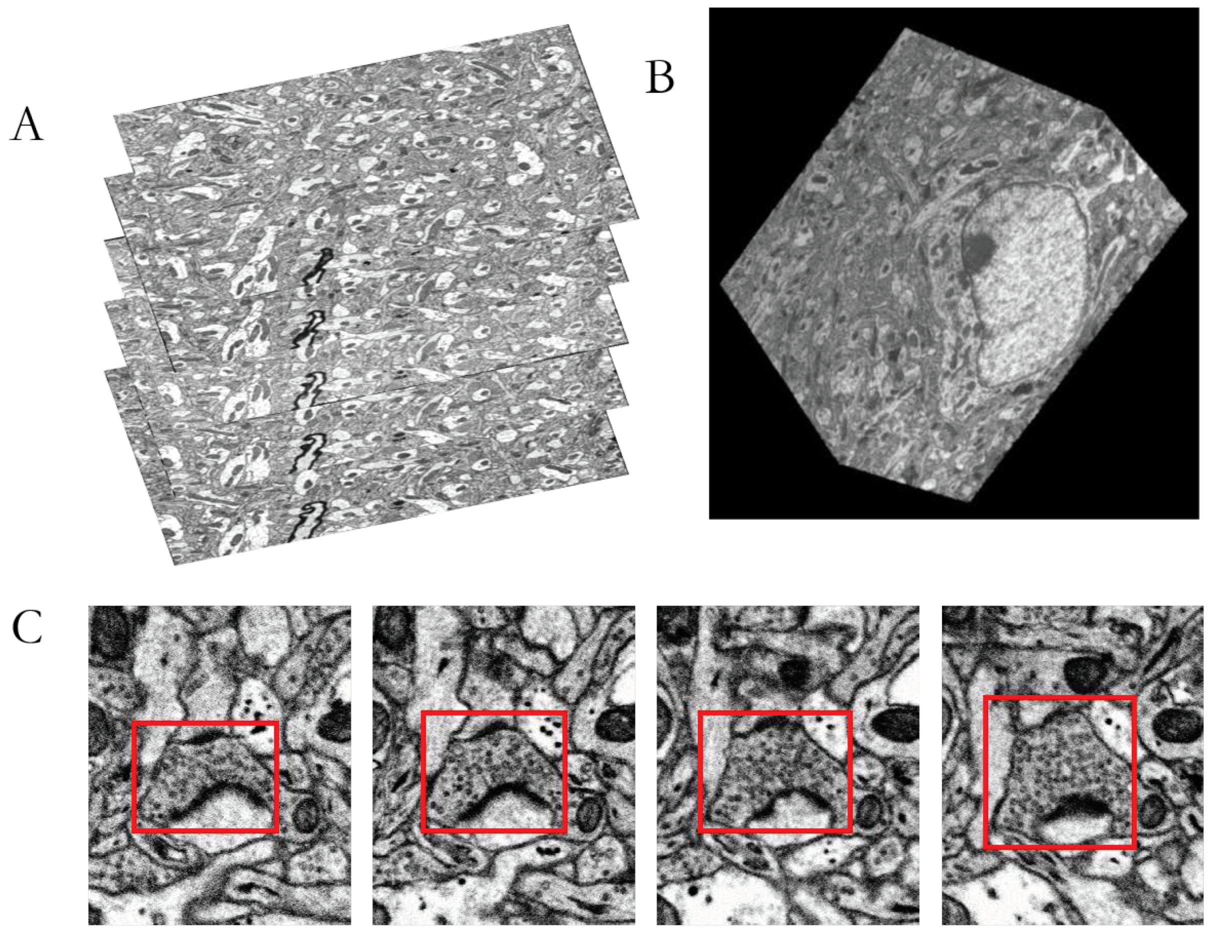
2. Materials
3. Methods
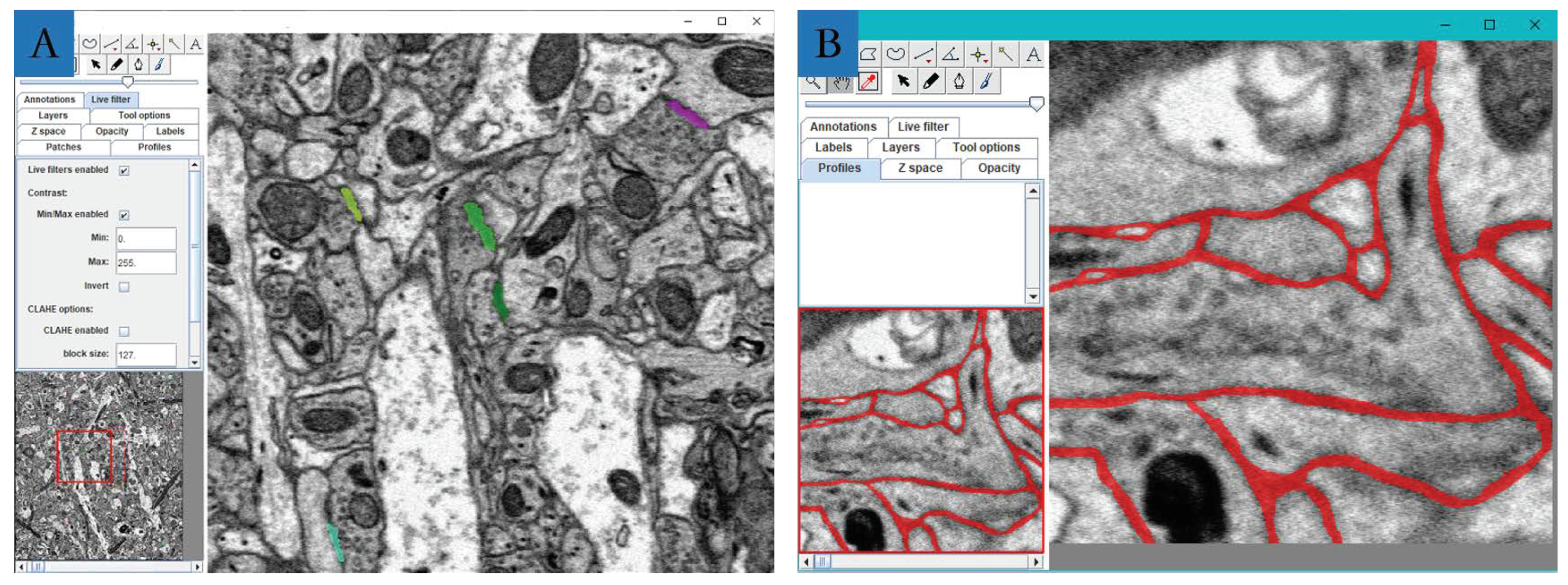
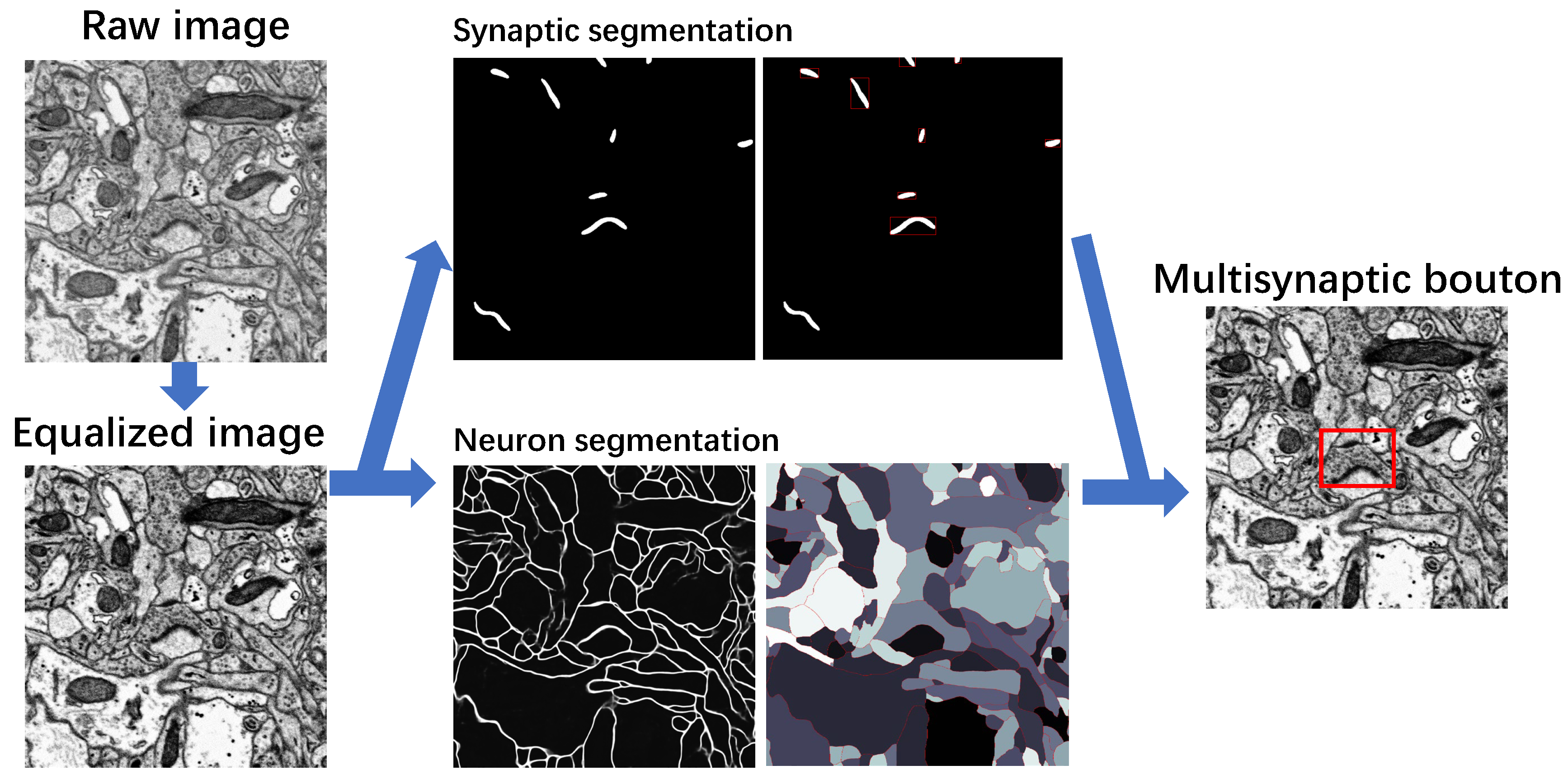
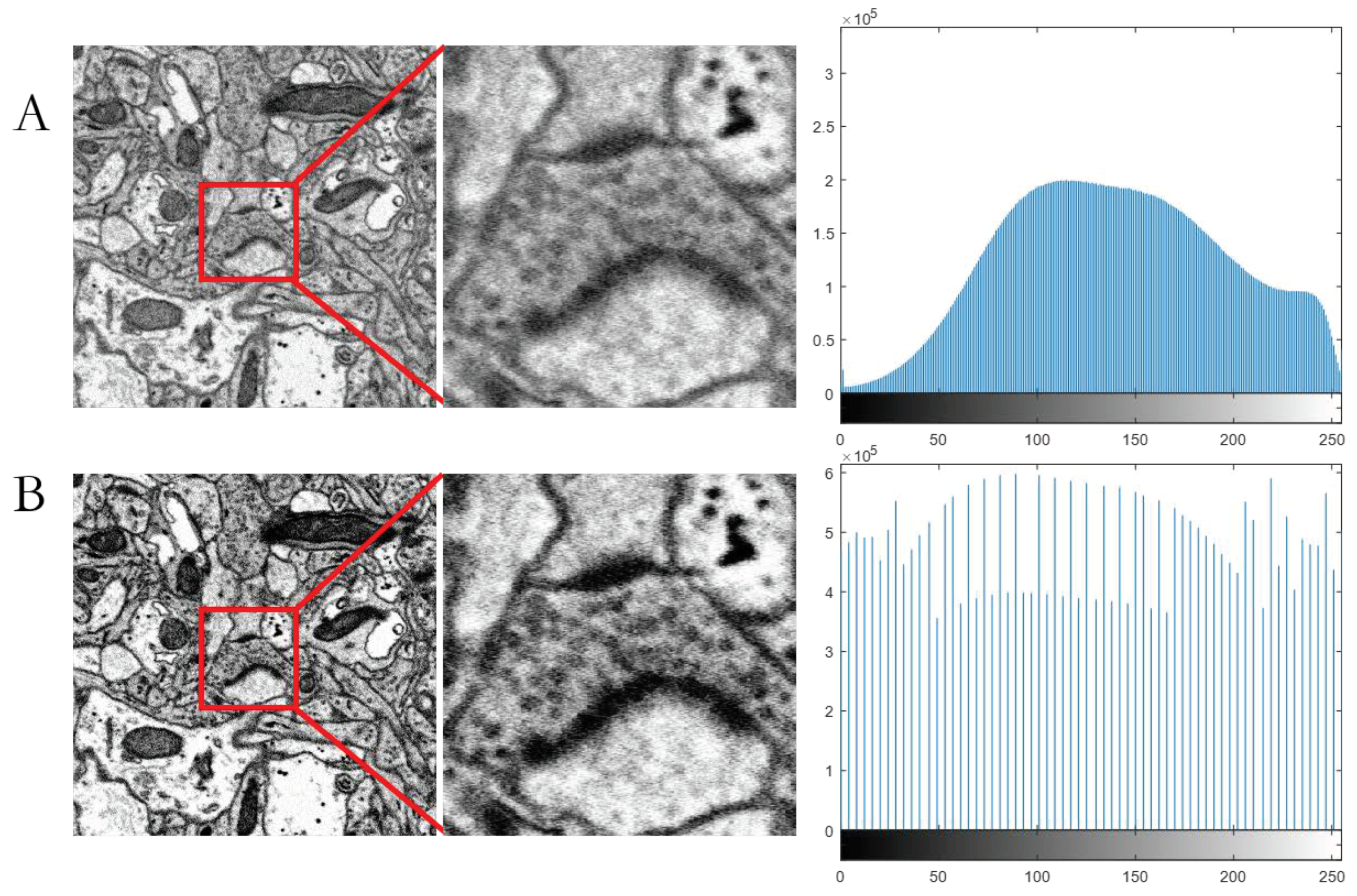
3.1. Image Preprocessing
3.2. Recognition of Synapse
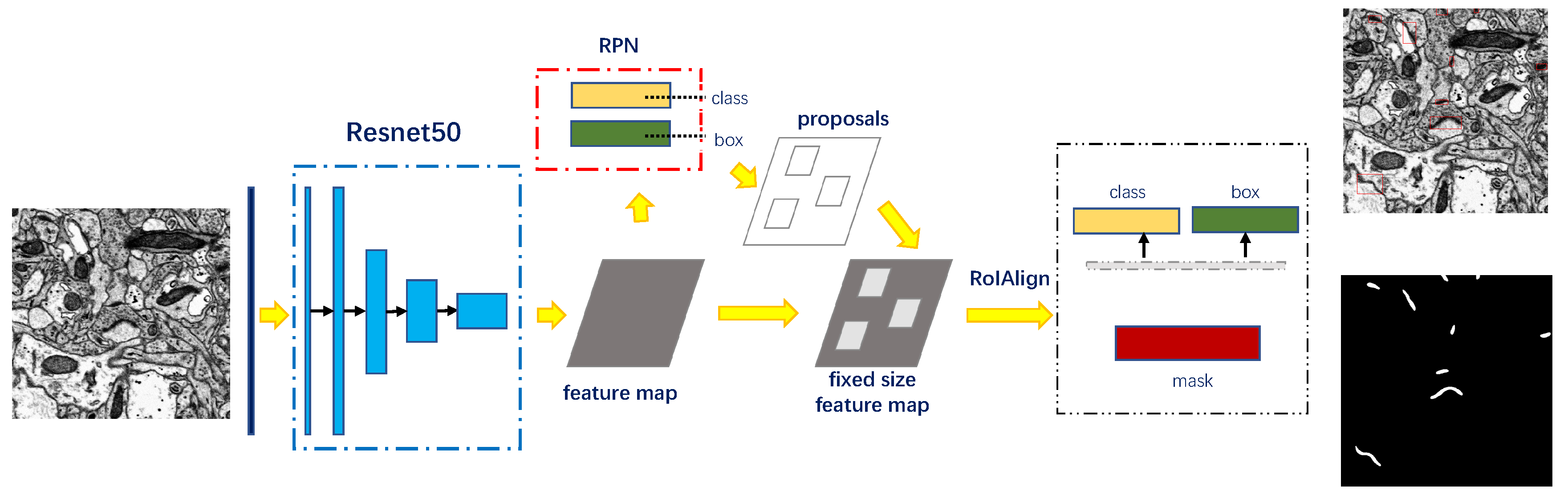
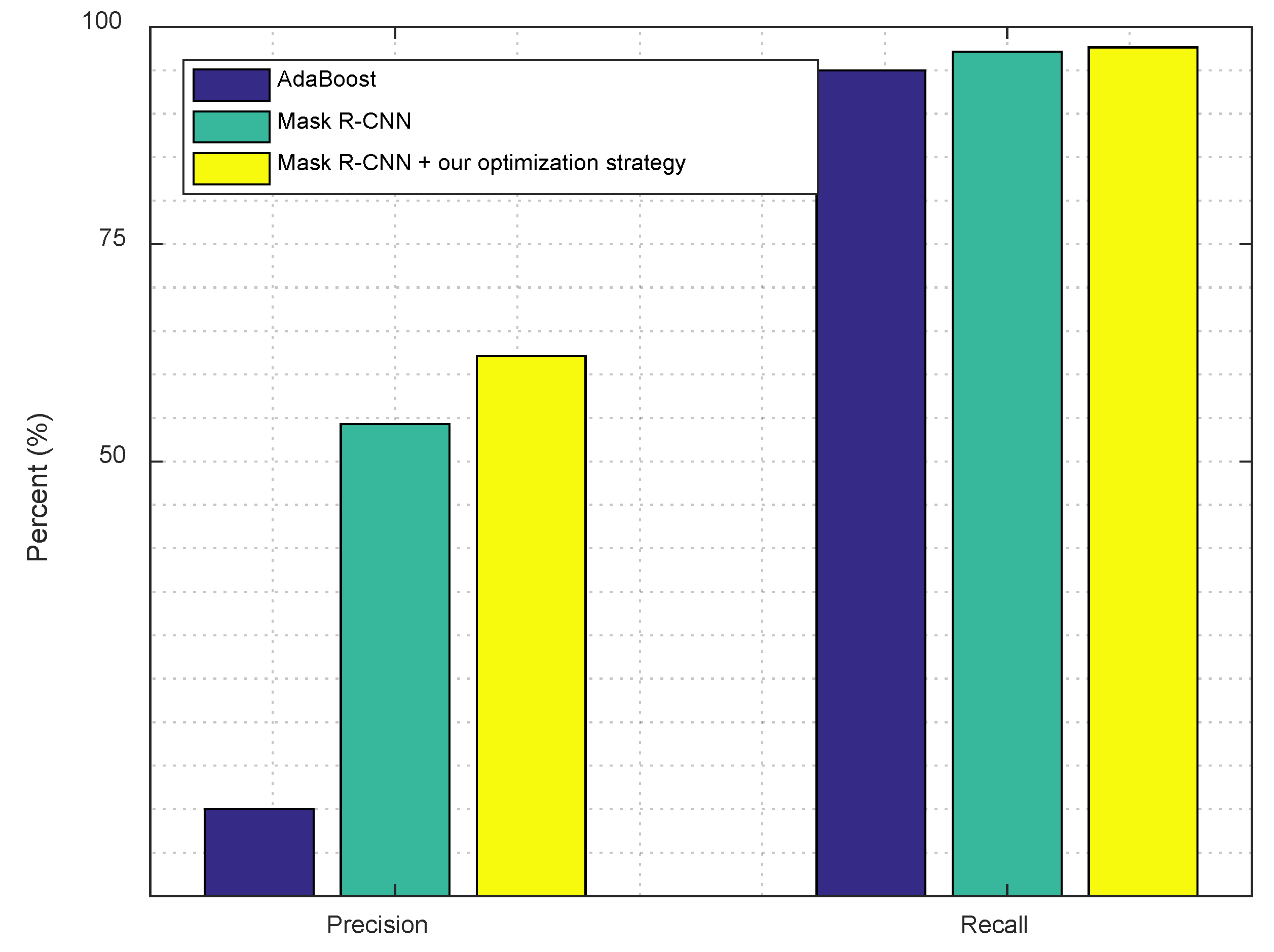
3.2.1. Detection and Segmentation with Mask R-CNN
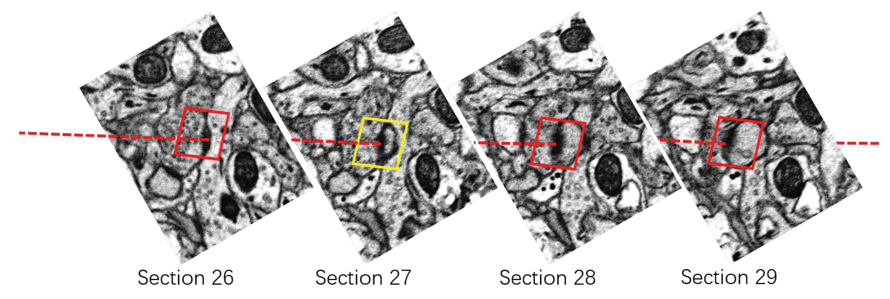
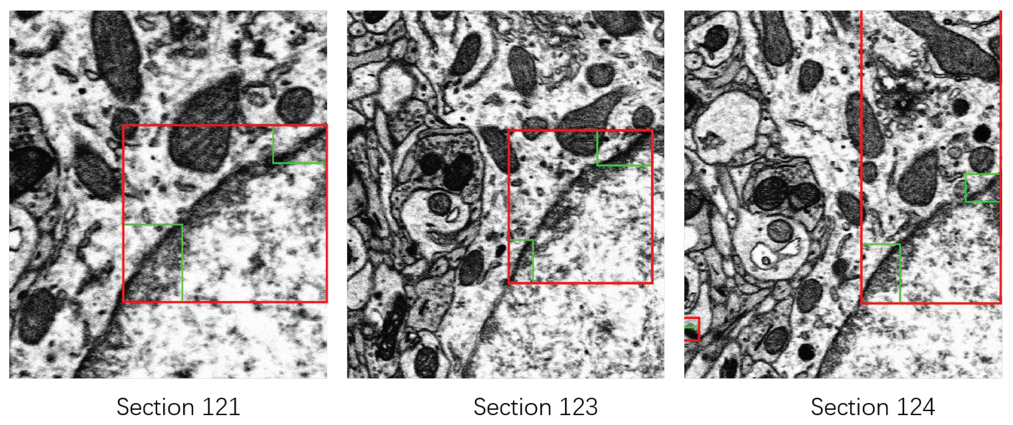
3.2.2. Rectifying Detection Results of Synapses on the Serial EM Image Stack
- For the synapse on the first section , we assign it a 3D serial number .
- For the synapse on the section , we calculate the Euclidean distance between and . Denote by the distance between and :where is the centroid of the bounding box of .
- Find the closest synapse to , and denote it by .
- Verify if is the closest synapse to on the section. Find the closest synapse to on the section, and denote it by .If and the distance between and is smaller than a given threshold (according to the thickness of sections of 50 nm, i.e., 25 pixels in the x-y direction, we set ),we consider that and are the same synapse appearing on different sections. Then, we assign the 3D serial number of to . If or Equation (6) is not satisfied, we consider that and are not the same synapse in the 3D perspective. We assign a new 3D serial number to .
3.3. Segmentation of Neuron
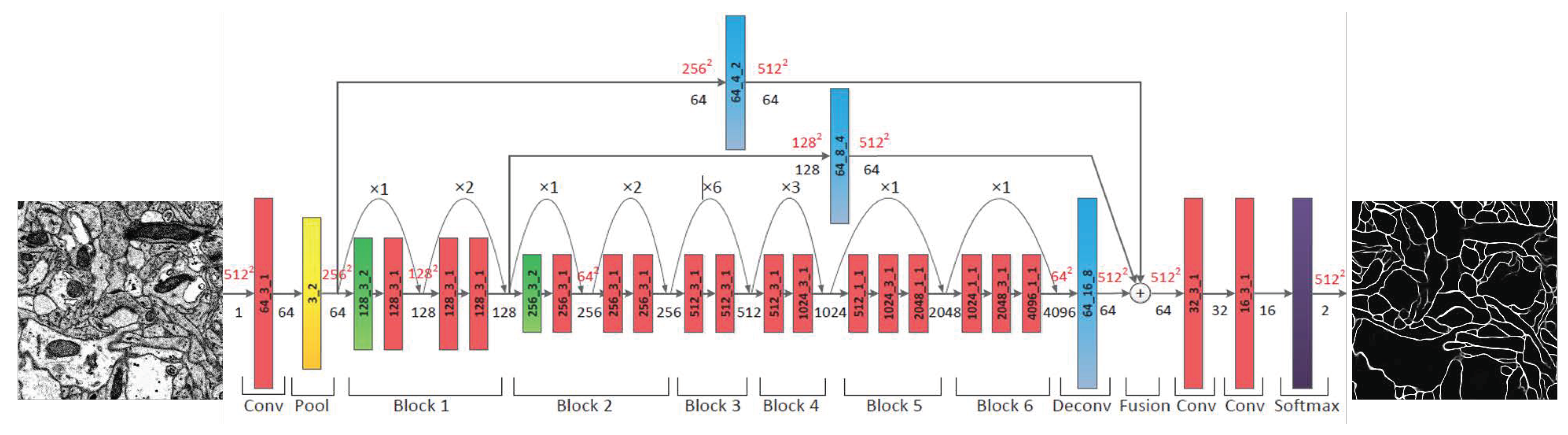
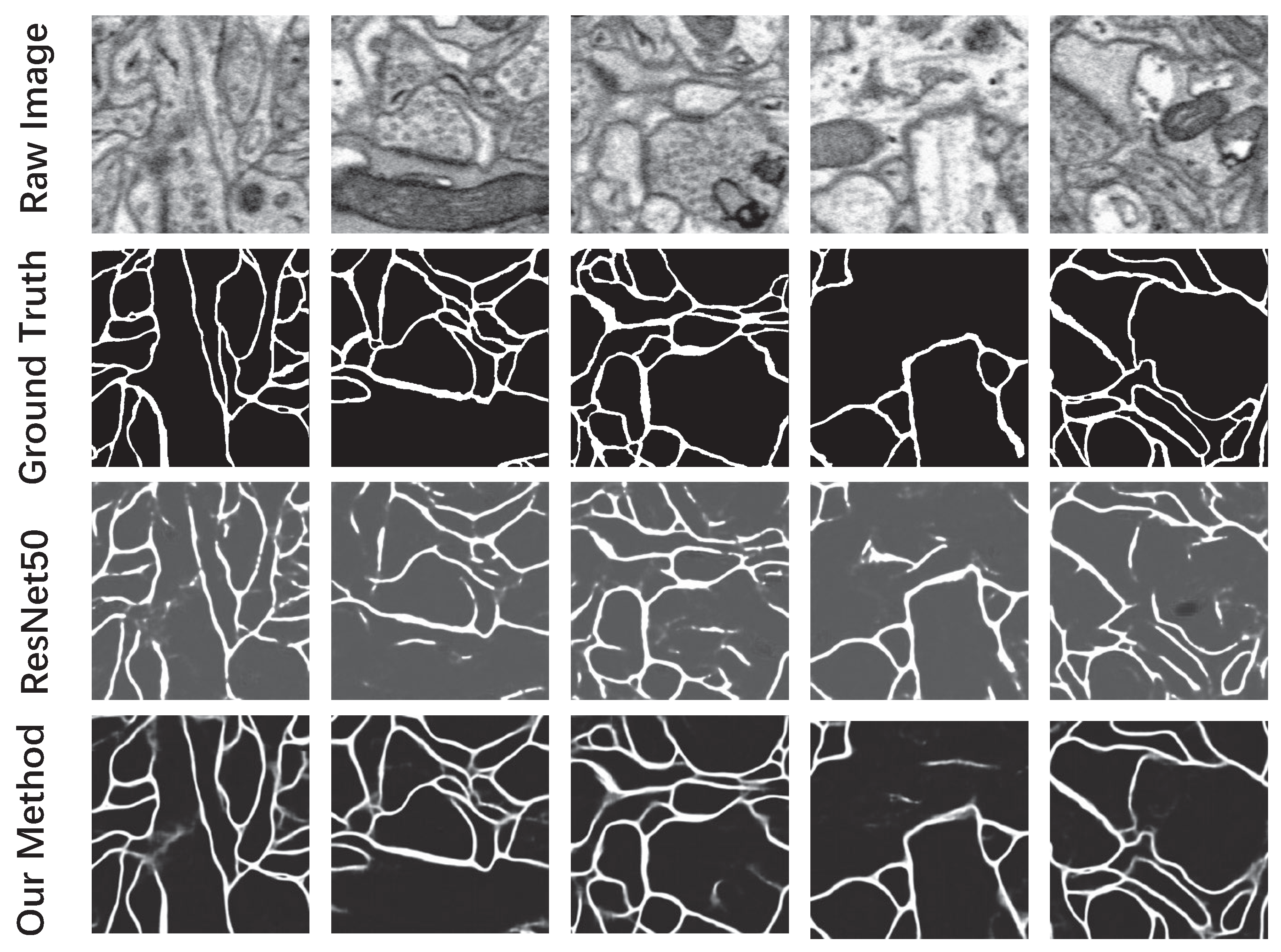
3.3.1. Probability Map of the Neuronal Membrane
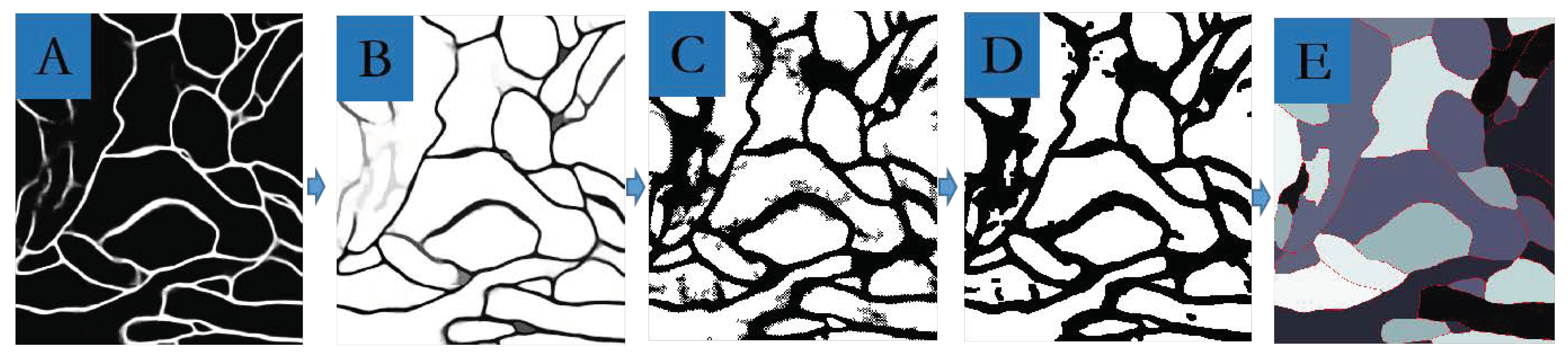
3.3.2. Neuron Segmentation with the Marker-Controlled Watershed Algorithm
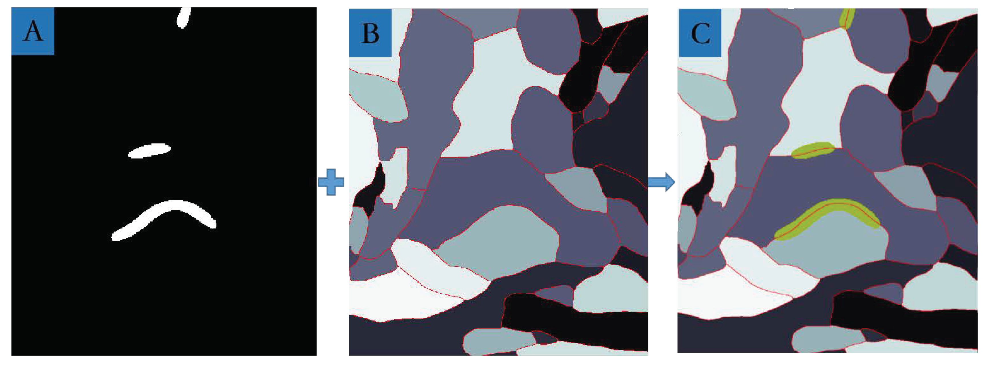
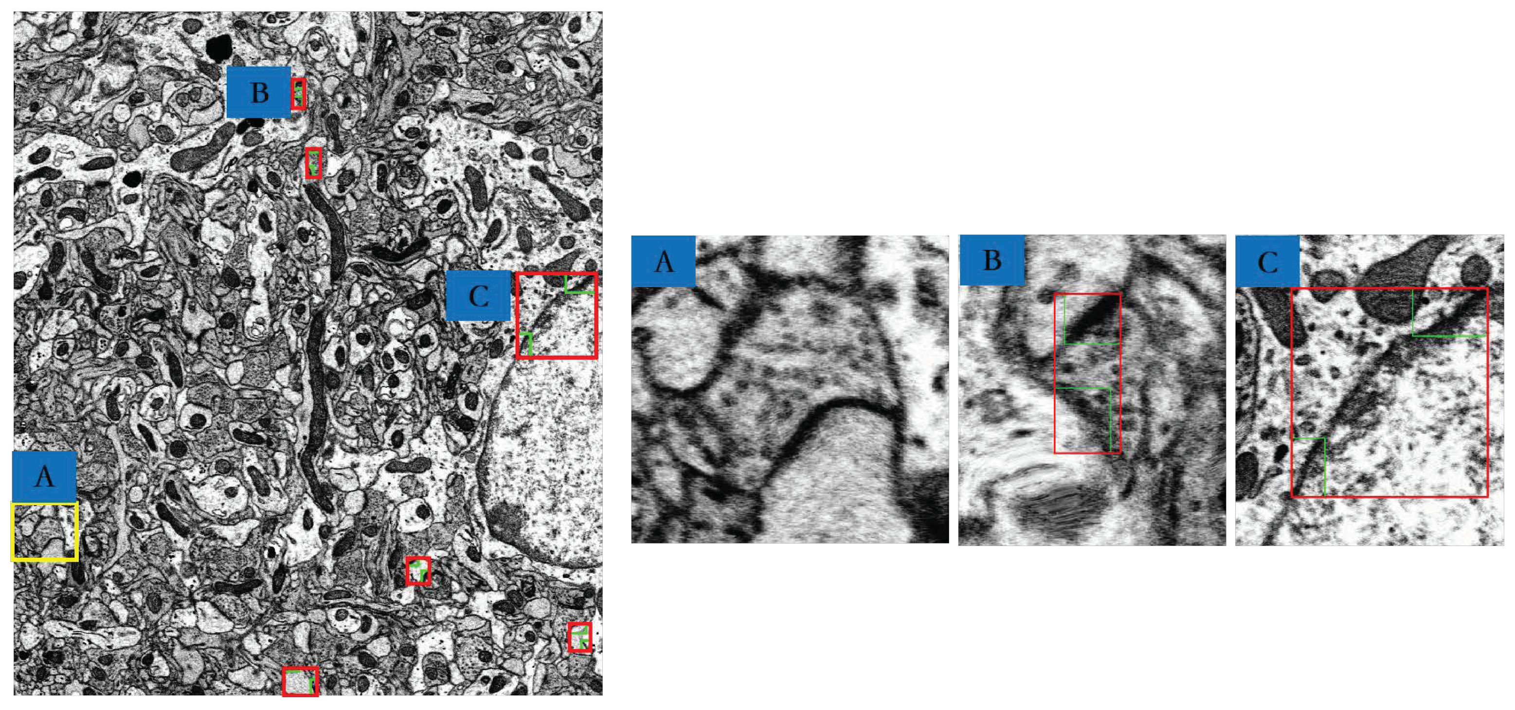
3.4. MSB Identification
4. Results
5. Discussion
6. Conclusions
Author Contributions
Funding
Acknowledgments
Conflicts of Interest
References
- Quan, T.; Hildebrand, D.G.; Jeong, W. Fusionnet: A deep fully residual convolutional neural network for image segmentation in connectomics. arXiv 2016, arXiv:1612.05360. [Google Scholar]
- Briggman, K.L.; Bock, D.D. Volume electron microscopy for neuronal circuit reconstruction. Curr. Opin. Neurobiol. 2012, 22, 154–161. [Google Scholar] [CrossRef] [PubMed]
- Januszewski, M.; Maitin-Shepard, J.; Li, P.; Kornfeld, J.; Denk, W.; Jain, V. High-precision automated reconstruction of neurons with flood-filling networks. arXiv 2016, arXiv:1611.00421. [Google Scholar] [CrossRef]
- Vitaladevuni, S.; Mishchenko, Y.; Genkin, A.; Chklovskii, D.; Harris, K. Mitochondria Detection in Electron Microscopy Images. In Workshop on Microscopic Image Analysis with Applications in Biology. 2008, Volume 42. Available online: https://webcache.googleusercontent.com/search?q=cache:XOIGQp_Yui8J:https://pdfs.semanticscholar.org/bde5/7551f74722159237d338ad961dae1847df76.pdf+&cd=1&hl=zh-CN&ct=clnk&gl=hk (accessed on 25 June 2019).
- Lucchi, A.; Smith, K.; Achanta, R.; Knott, G.; Fua, P. Supervoxel-based segmentation of mitochondria in em image stacks with learned shape features. IEEE Trans. Med. Imaging 2012, 31, 474–486. [Google Scholar] [CrossRef] [PubMed]
- Staffler, B.; Berning, M.; Boergens, K.M.; Gour, A.; van der Smagt, P.; Helmstaedter, M. SynEM, automated synapse detection for connectomics. Elife 2017, 6, e26414. [Google Scholar] [CrossRef]
- Xiao, C.; Li, W.; Deng, H.; Chen, X.; Yang, Y.; Xie, Q.; Han, H. Effective automated pipeline for 3D reconstruction of synapses based on deep learning. BMC Bioinform. 2018, 19, 263. [Google Scholar] [CrossRef] [PubMed]
- Friedlander, M.J.; Martin, K.A.; Wassenhove-Mccarthy, D. Effects of monocular visual deprivation on geniculocortical innervation of area 18 in cat. J. Neurosci. Off. J. Soc. Neurosci. 1991, 11, 3268. [Google Scholar] [CrossRef]
- Kea Joo, L.; In Sung, P.; Hyun, K.; Greenough, W.T.; Pak, D.T.S.; Im Joo, R. Motor skill training induces coordinated strengthening and weakening between neighboring synapses. J. Neurosci. Off. J. Soc. Neurosci. 2013, 33, 9794–9799. [Google Scholar]
- Jones, T.A.; Klintsova, A.Y.; Kilman, V.L.; Sirevaag, A.M.; Greenough, W.T. Induction of Multiple Synapses by Experience in the Visual Cortex of Adult Rats. Neurobiol. Learn. Mem. 1997, 68, 13–20. [Google Scholar] [CrossRef]
- Jones, E.G.; Powell, T.P. Morphological variations in the dendritic spines of the neocortex. J. Cell Sci. 1969, 5, 509–529. [Google Scholar]
- Toni, N.; Buchs, P.A.; Nikonenko, I.; Bron, C.R.; Muller, D. LTP promotes formation of multiple spine synapses between a single axon terminal and a dendrite. Nature 1999, 402, 421–425. [Google Scholar] [CrossRef] [PubMed]
- Yang, Y.; Liu, D.Q.; Huang, W.; Deng, J.; Sun, Y.; Zuo, Y.; Poo, M.M. Selective synaptic remodeling of amygdalocortical connections associated with fear memory. Nat. Neurosci. 2016, 19, 1348–1355. [Google Scholar] [CrossRef] [PubMed]
- Steward, O.; Vinsant, S.L.; Davis, L. The process of reinnervation in the dentate gyrus of adult rats: An ultrastructural study of changes in presynaptic terminals as a result of sprouting. J. Comp. Neurol. 1988, 267, 203–210. [Google Scholar] [CrossRef] [PubMed]
- Geinisman, Y.; Berry, R.W.; Disterhoft, J.F.; Power, J.M.; Van der Zee, E.A. Associative learning elicits the formation of multiple-synapse boutons. J. Neurosci. Off. J. Soc. Neurosci. 2001, 21, 5568–5573. [Google Scholar] [CrossRef]
- Yuko, H.; C Sehwan, P.; Janssen, W.G.M.; Michael, P.; Rapp, P.R.; Morrison, J.H. Synaptic characteristics of dentate gyrus axonal boutons and their relationships with aging, menopause, and memory in female rhesus monkeys. J. Neurosci. 2011, 31, 7737–7744. [Google Scholar]
- Zhou, W.; Li, H.; Zhou, X. 3D Dendrite Reconstruction and Spine Identification. In Proceedings of the International Conference on Medical Image Computing & Computer-assisted Intervention, New York, NY, USA, 6–10 September 2008. [Google Scholar]
- Moolman, D.L.; Vitolo, O.V.; Vonsattel, J.P.G.; Shelanski, M.L. Dendrite and dendritic spine alterations in alzheimer models. J. Neurocytol. 2004, 33, 377–387. [Google Scholar] [CrossRef] [PubMed]
- Eduard, K.; David, H.; Menahem, S. Dynamic regulation of spine-dendrite coupling in cultured hippocampal neurons. Eur. J. Neurosci. 2015, 20, 2649–2663. [Google Scholar]
- Fischer, M.; Kaech, S.; Knutti, D.; Andrew, M. Rapid Actin-Based Plasticity in Dendritic Spines. Neuron 1998, 20, 847–854. [Google Scholar] [CrossRef]
- Martinez-Cerdeno, V. Dendrite and spine modifications in autism and related neurodevelopmental disorders in patients and animal models. Dev. Neurobiol. 2017, 77, 393–404. [Google Scholar] [CrossRef]
- Segal, M.; Andersen, P. Dendritic spines shaped by synaptic activity. Curr. Opin. Neurobiol. 2000, 10, 582–586. [Google Scholar] [CrossRef]
- Matus, A. Actin-based plasticity in dendritic spines. Science 2000, 290, 754–758. [Google Scholar] [CrossRef]
- Wang, Y.; Yuan, Y.T.; Li, L.; Wang, J. Face recognition via collaborative representation based multiple one-dimensional embedding. Int. J. Wavelets Multiresolut. Inf. Process. 2016, 14, 1640003. [Google Scholar] [CrossRef]
- Xie, Q.; Chen, X.; Deng, H.; Liu, D.; Sun, Y.; Zhou, X.; Yang, Y.; Han, H. An automated pipeline for bouton, spine, and synapse detection of in vivo two-photon images. Biodata Min. 2017, 10, 40. [Google Scholar] [CrossRef] [PubMed]
- Hong, B.; Liu, J.; Li, W.; Xiao, C.; Xie, Q.; Han, H. Fully Automatic Synaptic Cleft Detection and Segmentation from EM Images Based on Deep Learning. In Proceedings of the International Conference on Brain Inspired Cognitive Systems, Xi’an, China, 7–8 July 2018; pp. 64–74. [Google Scholar]
- He, K.; Gkioxari, G.; Dollar, P.; Girshick, R. Mask R-CNN. IEEE Trans. Pattern Anal. Mach. Intell. 2017. [Google Scholar] [CrossRef]
- Li, W.; Liu, J.; Xiao, C.; Deng, H.; Xie, Q.; Han, H. A fast forward 3D connection algorithm for mitochondria and synapse segmentations from serial EM images. BioData Min. 2018, 11, 24. [Google Scholar] [CrossRef]
- Xiao, C.; Liu, J.; Chen, X.; Han, H.; Shu, C.; Xie, Q. Deep contextual residual network for electron microscopy image segmentation in connectomics. In Proceedings of the IEEE International Symposium on Biomedical Imaging, Washington, DC, USA, 4–7 April 2018; pp. 378–381. [Google Scholar]
- Liu, H.; Chen, Z.; Xie, C. Multiscale morphological watershed segmentation for gray level image. Int. J. Wavelets Multiresolut. Inf. Process. 2008, 4, 627–641. [Google Scholar] [CrossRef]
- Neumann, U.; Riemenschneider, M.; Sowa, J.P.; Baars, T.; Kalsch, J.; Canbay, A.; Heider, D. Compensation of feature selection biases accompanied with improved predictive performance for binary classification by using a novel ensemble feature selection approach. Biodata Min. 2016, 9, 36. [Google Scholar] [CrossRef]
- Unnikrishnan, R.; Pantofaru, C.; Hebert, M. Toward objective evaluation of image segmentation algorithms. IEEE Trans. Pattern Anal. Mach. Intell. 2007, 6, 929–944. [Google Scholar] [CrossRef]
- Lamb, A.; Binas, J.; Goyal, A.; Serdyuk, D.; Subramanian, S.; Mitliagkas, I.; Bengio, Y. Fortified networks: Improving the robustness of deep networks by modeling the manifold of hidden representations. arXiv 2018, arXiv:1804.02485. [Google Scholar]
- Unger, M.; Pock, T.; Bischof, H. Continuous globally optimal image segmentation with local constraints. In Computer Vision Winter Workshop. 2008, Volume 2008. Available online: https://www.semanticscholar.org/paper/Continuous-Globally-Optimal-Image-Segmentation-with-Unger-Pock/2781ccb8c9e8135b6063b19d117901b91b8d2fdd (accessed on 25 June 2019).
- Roberts, M.; Jeong, W.K.; Vázquez-Reina, A.; Unger, M.; Bischof, H.; Lichtman, J.; Pfister, H. Neural process reconstruction from sparse user scribbles. In Proceedings of the International Conference on Medical Image Computing and Computer-Assisted Intervention, Toronto, ON, Canada, 18–22 September 2011; pp. 621–628. [Google Scholar]
- Li, W.; Deng, H.; Rao, Q.; Xie, Q.; Chen, X.; Han, H. An automated pipeline for mitochondrial segmentation on atum-sem stacks. J. Bioinform. Comput. Biol. 2017, 15, 1750015. [Google Scholar] [CrossRef]
- He, K.; Zhang, X.; Ren, S.; Sun, J. Deep residual learning for image recognition. In Proceedings of the IEEE Conference on Computer Vision and Pattern Recognition, Las Vegas, NV, USA, 27–30 June 2016; pp. 770–778. [Google Scholar]
- Geinisman, Y. Structural synaptic modifications associated with hippocampal LTP and behavioral learning. Cerebral Cortex 2000, 10, 952–962. [Google Scholar] [CrossRef] [PubMed]
- Lalo, U.; Palygin, O.; Verkhratsky, A.; Grant, S.G.; Pankratov, Y. ATP from synaptic terminals and astrocytes regulates NMDA receptors and synaptic plasticity through PSD-95 multi-protein complex. Sci. Rep. 2016, 6, 33609. [Google Scholar] [CrossRef] [PubMed]
- Kim, H.W.; Oh, S.; Lee, S.H.; Lee, S.; Na, J.E.; Lee, K.J.; Rhyu, I.J. Different types of multiple-synapse boutons in the cerebellar cortex between physically enriched and ataxic mutant mice. Microsc. Res. Tech. 2018, 82, 25–32. [Google Scholar] [CrossRef] [PubMed]


| Morphology Method | Variational Model Method [34,35,36] | Mask R-CNN | |
|---|---|---|---|
| J(Synapses, Ground truth) | 19.21% | 18.49% | 65.55% |
| Our Method | ResNet50 [37] | |
|---|---|---|
| Pixel-error | 5.61% | 7.81% |
| Rand-error [32] | 12.74% | 27.34% |
| Image | Manual | Our Method | ||
|---|---|---|---|---|
| Total | False Positive | False Negative | ||
| Layer 1 | 8 | 10 | 2 | 0 |
| Layer 21 | 7 | 10 | 3 | 0 |
| Layer 41 | 6 | 7 | 1 | 0 |
| Layer 61 | 3 | 5 | 2 | 0 |
| Layer 81 | 3 | 4 | 2 | 1 |
| Layer 101 | 4 | 7 | 3 | 0 |
| Layer 121 | 5 | 6 | 2 | 1 |
| Layer 141 | 4 | 7 | 4 | 1 |
| Layer 161 | 8 | 11 | 3 | 0 |
| Layer 178 | 3 | 3 | 0 | 0 |
| Average | 5.1 | 7 | 2.2 | 0.3 |
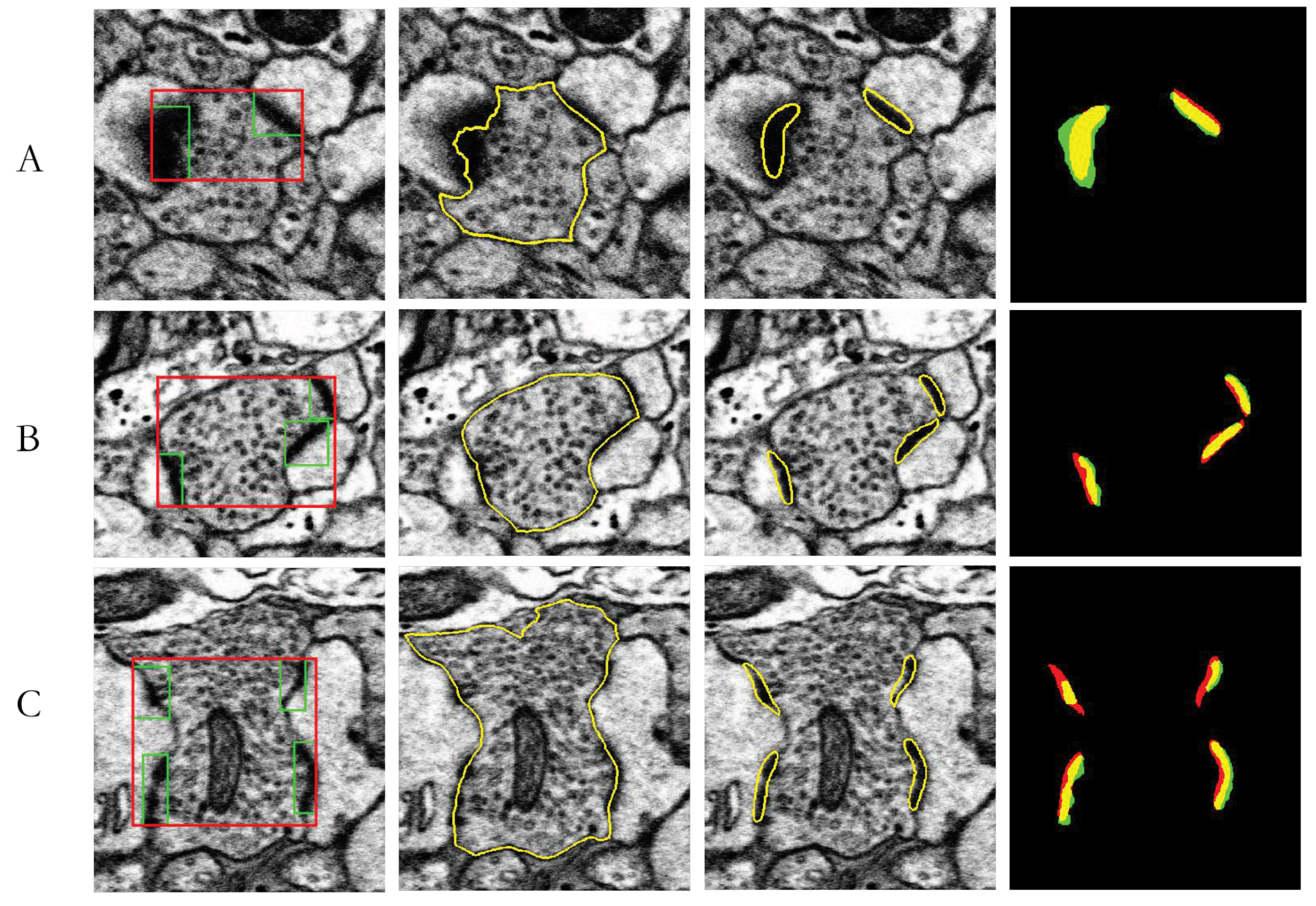
| J(Synapses, Ground truth) | Area(Neuron) (µm2) | Area(Synapse) (µm2) | Area(Neuron)/Area(Synapses) | |
|---|---|---|---|---|
| A | 62.54% | 0.2050 | 0.0266 | 12.98% |
| B | 57.48% | 0.3634 | 0.0334 | 9.20% |
| C | 48.40% | 0.6497 | 0.0048 | 7.40% |
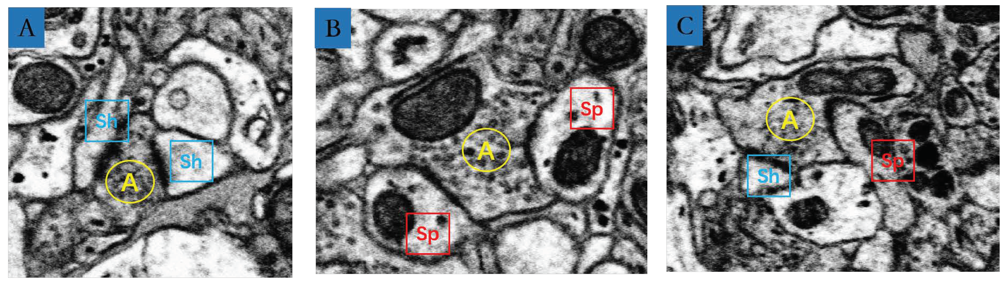
| Type A | Type B | Type C | Total | |
|---|---|---|---|---|
| Numbers | 946 | 50 | 7 | 1003 |
| Ratio | 94.31% | 4.99% | 0.7% | 100% |
© 2019 by the authors. Licensee MDPI, Basel, Switzerland. This article is an open access article distributed under the terms and conditions of the Creative Commons Attribution (CC BY) license (http://creativecommons.org/licenses/by/4.0/).
Share and Cite
Deng, H.; Ma, C.; Han, H.; Xie, Q.; Shen, L. A Method for Identification of Multisynaptic Boutons in Electron Microscopy Image Stack of Mouse Cortex. Appl. Sci. 2019, 9, 2591. https://doi.org/10.3390/app9132591
Deng H, Ma C, Han H, Xie Q, Shen L. A Method for Identification of Multisynaptic Boutons in Electron Microscopy Image Stack of Mouse Cortex. Applied Sciences. 2019; 9(13):2591. https://doi.org/10.3390/app9132591
Chicago/Turabian StyleDeng, Hao, Chao Ma, Hua Han, Qiwei Xie, and Lijun Shen. 2019. "A Method for Identification of Multisynaptic Boutons in Electron Microscopy Image Stack of Mouse Cortex" Applied Sciences 9, no. 13: 2591. https://doi.org/10.3390/app9132591
APA StyleDeng, H., Ma, C., Han, H., Xie, Q., & Shen, L. (2019). A Method for Identification of Multisynaptic Boutons in Electron Microscopy Image Stack of Mouse Cortex. Applied Sciences, 9(13), 2591. https://doi.org/10.3390/app9132591