Research on Measurement Technology of Thermophysical Properties for Full-Scale Phase Change Material Product in a Container

Featured Application

This paper proposed a method to measure the thermophysical properties for full-scale phase change material product which can be used in the field of temperature control. It is helpful to determine the temperature control performance of the full-scale phase change material products.

Abstract

The thermophysical properties of phase change material include thermal conductivity, heat of absorption, and phase change temperature range. This paper investigates the measurement methods of thermophysical properties for phase change material inside a full-scale container. The influence of contact thermal resistance is considered in a thermal conductivity test, and the formula for calculating the thermal conductivity of a phase change material inside the full-scale container is derived. In addition, the heat of absorption is measured based on the calibration results of the correction coefficient for heat flux sensors. In order to verify the reliability of the measurement method, the thermophysical properties of docosane and erythritol inside a full-scale specimen are measured, and the results are compared with HotDisk analyzer results and published data. The comparison results reveal that the method proposed in this paper can accurately measure the thermophysical properties of phase change material inside a full-scale specimen.

1. Introduction

With the development of science and technology, energy storage technology has been widely used in many practical applications [1,2,3,4,5]. In order to optimize the design of energy storage systems, it is important to accurately measure the thermophysical properties of a phase change material (PCM) used in an energy storage system, including the thermal conductivity, the heat of absorption, and the temperature range of the phase change. Furthermore, for a full-scale PCM product, it is necessary to measure the thermophysical properties of a PCM inside its container to determine whether the product is qualified. Therefore, an appropriate measurement method is needed.

For the measurement of thermal conductivity for a solid PCM, the hot wire method [6,7,8], the HotDisk method [9,10,11], and the steady state method [12,13,14] are widely used. In addition, the steady state method, including the heat flow method analysis (HFMA) method, is generally used to measure the thermal conductivity of a full-scale product. However, the steady state method is susceptible to the influence of contact thermal resistance [15]. In order to minimize the impact of thermal contact resistance, a flexible material with a high thermal conductivity is added to the specimen, hot plate, and cold plate. Silicone grease is the most widely used material to reduce contact thermal resistance [16]. However, the maximum operating temperature of silicone grease is 300 °C, which limits the temperature range of a thermal conductivity measurement. Moreover, after heating, silicone grease will pollute the specimen, hot plate, and cold plate. Therefore, a compensation method is needed to reduce the impact of contact thermal resistance without polluting the specimen so as to achieve an accurate measurement of thermal conductivity.

For the measurement of the heat of absorption and the temperature range of the phase change, differential scanning calorimetry (DSC) is widely used. For instance, Sun et al. [17] measured the melting temperature and enthalpy variations of n-octadecane paraffin and calcium chloride hexahydrate. Jiang et al. [18] tested the melting point and latent heat of Na₂CO₃–NaCl eutectic salt. This method requires very small samples of about 1–10 mg. Though it is possible to estimate the heat of absorption of a pure PCM during phase change process [19], it is obviously inappropriate for widely used composite materials. In order to test the heat of absorption of a larger specimen during the phase change process, Zhang et al. [20] proposed a temperature reference method called the T-history method. This method measures the phase change temperature range and latent heat of a PCM by comparing the step cooling temperature curve of a PCM with that of a comparative specimen. Several researchers improved this method in recent years [21,22,23]. Compared with the DSC method, this method requires larger samples of about 15 g.

However, in practical applications, an appropriate method is still needed to measure the heat of absorption and phase change temperature range of a full-scale PCM product, even in a container. In 2012, based on the American Standard Test Method (ASTM) C518, Shukla et al. [24] proposed a new method called the dynamic heat flow meter analysis (DHFMA) method to measure the PCM content in gypsum board. Then, several researchers focused on this method, and a new ASTM standard called ASTM C1784 was established. Kosny et al. [25] carried out experimental and theoretical analyses on this method to measure the heat of absorption of fiber insulation materials containing a microcapsule PCM. In 2018, Biswas et al. [26] studied the thermal storage characteristics of two PCM-containing qualitative building materials by using this method, and they determined the temperature-dependent enthalpy functions for phase change.

This paper presents a measurement of thermal conductivity for a solid PCM in a container using the HFMA method with contact thermal resistance compensation; it also presents the phase change temperature range and heat of absorption measurements for a PCM in a container using the DHFMA method. The measurement methods for solid thermal conductivity and heat of absorption of a PCM product are established, and the calculation methods for solid thermal conductivity and heat of absorption of a PCM are deduced. Through the calibration of the sensitivity coefficient and correction coefficient for the heat of absorption of heat flux meter that varies with temperature, and the calibration of contact thermal resistance that varies with temperature, the thermophysical parameters of PCM can be accurately measured.

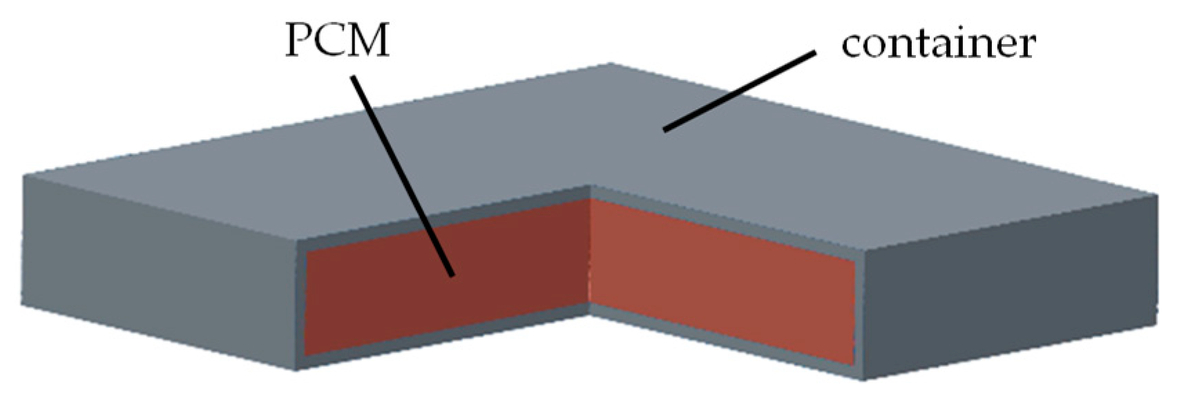
2. Measurement Method of Thermophysical Parameters for PCM in the Container

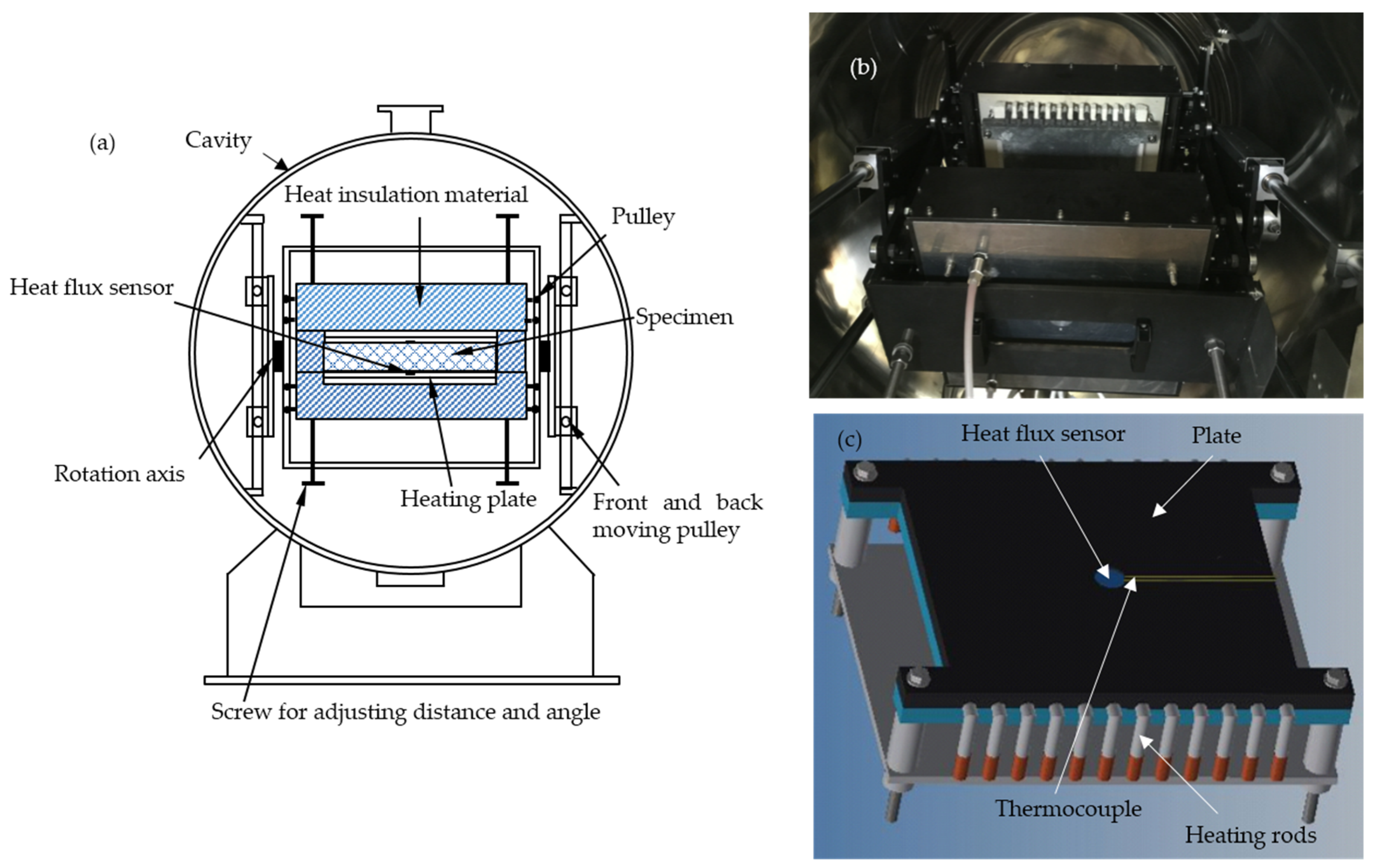
2.1. Measurement Apparatus

Figure 1a,b shows the diagrammatic sketch and photograph of the measurement apparatus which is design and constructed by our team, respectively [27]. The apparatus consisted of upper and lower plates with the same structures. The plates were made of silicon carbide (SiC), which has a large thermal conductivity in order to ensure temperature uniformity. A heat flux sensor and a thermocouple were placed on the center of the surface of each plate, as shown in Figure 1c. The model of the heat flux sensor was HT-50, which was purchased from the International Thermal Instrument Company (Del Mar, CA, USA). It is a conductive plate heat flux sensor with a diameter of 15.9 mm and a thickness of 3.5 mm. During the measurement, a test specimen with a dimension of 300 mm × 300 mm × 50 mm was sandwiched between the two plates, and its sides were insulated by thermal insulation cotton. In the measurement of thermal conductivity, one plate was heated, while, in the measurement of heat of absorption, both plates were heated to the same temperature.

A specimen made of 304L stainless steel with dimensions of 300 mm × 300 mm × 50 mm was used as the calibration specimen. In the testing experiment, a container, made of 304L stainless steel with same surface processing as the calibration material, was filled with a PCM. The pressure on the container filled with the PCM during the experiment was the same as that on the calibration specimen. The thickness of the container’s envelope was 5 mm. Figure 2 shows the 3D diagram and cross section of the testing specimen.

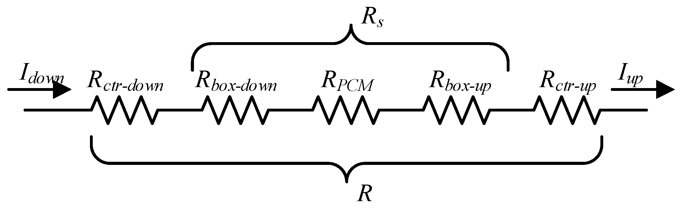
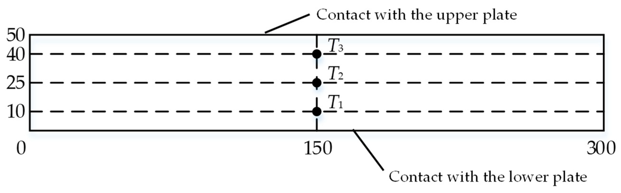
2.2. HFMA Method of PCM in the Container Considering Contact Thermal Resistance

The HFMA method is based on Fourier’s law for calculating the thermal conductivity of solid material. More than one heat flux meter should be used in this method to obtain the heat flux across the specimen. Then, the thermal conductivity is expressed as

$$\lambda =\frac{q\times \delta }{\Delta T}$$

(1)

in which q is the heat flow measured by heat flux meter, δ represents the thickness of the specimen, and ΔT is the temperature difference between two ends of the specimen. The thermal resistance of the specimen is expressed in Equation (2).

$$R=\frac{\Delta T}{q}=\frac{\delta }{\lambda }$$

(2)

Compared with the formula of Ohm’s law in circuits, the total thermal resistance between the hot plate and the cold plate is shown in Figure 3, in which I_down = I_up represents the heat flow between the two plates, R_ctr is the contact thermal resistance between the specimen and the plate, R_box is the thermal resistance of container material, and R_PCM is the thermal resistance of the PCM inside the container. In addition, the PCM is put into the container when it is in liquid phase. Then, the container is placed vertically during the solidification process of the PCM, which makes the PCM fully touch with the wall of the container. Therefore, the contact thermal resistance between the PCM and the container is neglected.

Based on the traditional steady-state method, the total thermal resistance between the hot plate and the cold plate, R, is expressed in Equation (3), in which R_s is the thermal resistance of the full-scale specimen (as shown in Equation (4)).

$$R=R_{ctr-down}+R_s+R_{ctr-up}$$

(3)

$$R_s=R_{box-down}+R_{PCM}+R_{box-up}$$

(4)

The thermal conductivity of the container wall is measured by a HotDisk analyzer, and the thermal resistance of the container wall is calculated by Equation (5).

$$R_{box-down}+R_{box-up}=\frac{{\delta }_{box-down}+{\delta }_{box-up}}{{\lambda }_{box}}$$

(5)

Then, the calculation model of R_PCM is deduced, as shown in Equation (6), in which R_ctr-down and R_ctr-up are calibrated functions that vary with temperature.

$$R_{PCM}=R-R_{ctr-down}-R_{ctr-up}-\frac{{\delta }_{box-down}+{\delta }_{box-up}}{{\lambda }_{box}}$$

(6)

Therefore, the thermal conductivity of the PCM in the container can be obtained in Equation (7).

$${\lambda }_{PCM}=\frac{{\delta }_{PCM}}{R_{PCM}}$$

(7)

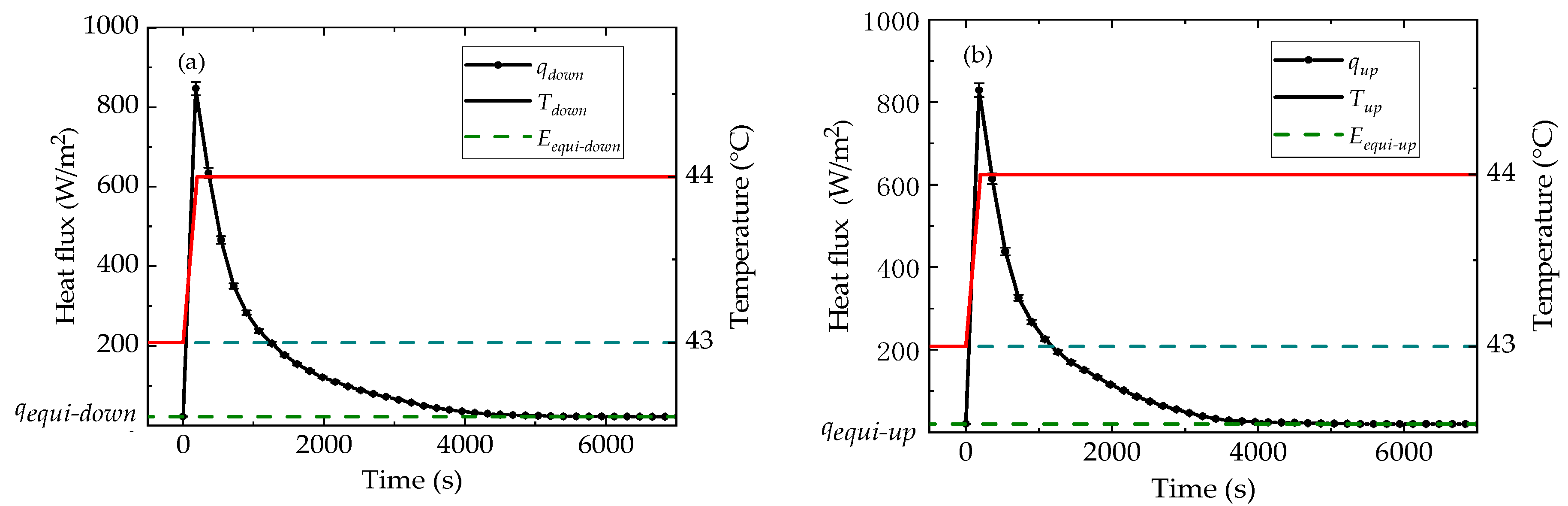
2.3. DHFMA Method of PCM in the Container

In the DHFMA method, the specimen is in thermal equilibrium at the beginning and the end of each temperature step. After considering the correction coefficient of the heat flux sensors, the integral of heat flow in each step can be calculated as the heat of absorption in each temperature step. Based on ASTM C1784, two heat flux sensors are used. When the temperature of the specimen changes from T_a to T_b, the change of areal enthalpy h_A can be obtained by measuring the values of both heat flux sensors installed on the two plates, as shown in Equation (8).

$$h_A\left(T_a,T_b\right)={\displaystyle \sum _{i=1}^n{S}_{up}\left(E_{i-up}-E_{equi-up}\right)\Delta \tau }+{\displaystyle \sum _{i=1}^n{S}_{down}\left(E_{i-down}-E_{equi-down}\right)\Delta \tau }$$

(8)

in which S is the sensitivity coefficient of the heat flux sensor after calibration, E represents the output voltage value of the heat flux sensor, and Δτ is the time interval. E_equi represents the value of heat flow returning to the steady state after loading the temperature step. In theory, if the heating plates and the specimen are well insulated, the E_equi will be zero when the value of heat flow returns to the steady state. However, in the experiment, it was impossible to achieve complete insulation. As such, the E_equi was near zero but not equal to zero. At the same time, the subscript up represents the heating plate on the top, while the subscript down represents the heating plate on the bottom.

Because the areal enthalpy of the heat flux sensor is not linear in the whole temperature range, the correction coefficient S_HFM (T_a,T_b) needs to be calibrated. Then, the areal enthalpy of the specimen (h_As (T_a,T_b)) can be calculated in Equation (9), which contains the areal enthalpy of the container and the PCM. In addition, the volume specific heat within each temperature step is considered to be linear, so the volume specific heat of the specimen with the container at the average temperature (Equation (10)) is obtained, which is shown in Equation (11).

$$h_{As}\left(T_a,T_b\right)=h_A\left(T_a,T_b\right)-{\displaystyle {\int }_{T_a}^{T_b}{S}_{HFM}\left(T_a,T_b\right)}\mathrm{d}T$$

(9)

$$T_{mean}=\frac{1}{2}\times \left(T_a+T_b\right)$$

(10)

$$C_V\left(T_{mean}\right)=\frac{h_{As}\left(T_a,T_b\right)}{\delta \times \left(T_b-T_a\right)}$$

(11)

In order to obtain the heat of absorption of the PCM in the container, further calculation is needed. Since the volume of a PCM changes during the phase change, the specific heat of a PCM is expressed by mass specific heat. Firstly, the heat of absorption of full-scale specimen is expressed in Equation (12), and the heat of absorption of the container is calculated by Equation (13), where the volume specific heat of the container (C_V-box (T)) is measured by a HotDisk analyzer with an accuracy of 7%. V_s refers to the volume of the full-scale specimen, and V_box is the volume of the container’s wall. Therefore, Equation (14) gives the mass specific heat of the PCM inside the full-scale container, in which m_PCM refers to the mass of the PCM. When a PCM is in the liquid or solid phase, C_m-PCM refers to the sensible specific heat of a PCM.

$$Q_s\left(T_a,T_b\right)=V_s\times {\displaystyle {\int }_{T_a}^{T_b}{C}_V}\left(T\right)\mathrm{d}T$$

(12)

$$Q_{box}\left(T_a,T_b\right)=V_{box}\times {\displaystyle {\int }_{T_a}^{T_b}{C}_{V-box}}\left(T\right)\mathrm{d}T$$

(13)

$$C_{m-PCM}\left(T_{mean}\right)=C_{m-PCM}\left(T_a,T_b\right)=\frac{Q_s\left(T_a,T_b\right)-Q_{box}\left(T_a,T_b\right)}{m_{PCM}\times \left(T_b-T_a\right)}$$

(14)

In addition, the latent heat of the PCM inside the full-scale container needs to be calculated and compared with the DSC test result to verify the rationality of this method. Through the non-linear fitting of the test points of the solid and liquid phases, the fitting results can be used as the baseline in the phase transition interval. The baseline is regarded as the sensible heat of the PCM in the phase change range, so the latent enthalpy of the PCM is expressed by Equation (15).

$$L={\displaystyle \sum _{T_a}^{T_b}\left(h_{PCM}-h_{sensible}\right)}$$

(15)

The linear fitting of the heat of absorption at different temperature steps in the solid phase is used as the baseline of the solid phase region. When the heat of absorption in a temperature step deviates from the baseline, the average temperature of this temperature step is regarded as the starting point of phase change, which is named T_a. Similarly, the linear fitting of the liquid phase is used as the baseline of the liquid phase region. When the heat of absorption in a temperature step returns to the liquid phase baseline, the average temperature of the temperature range is used as the phase transition termination point T_b.

3. Calibration

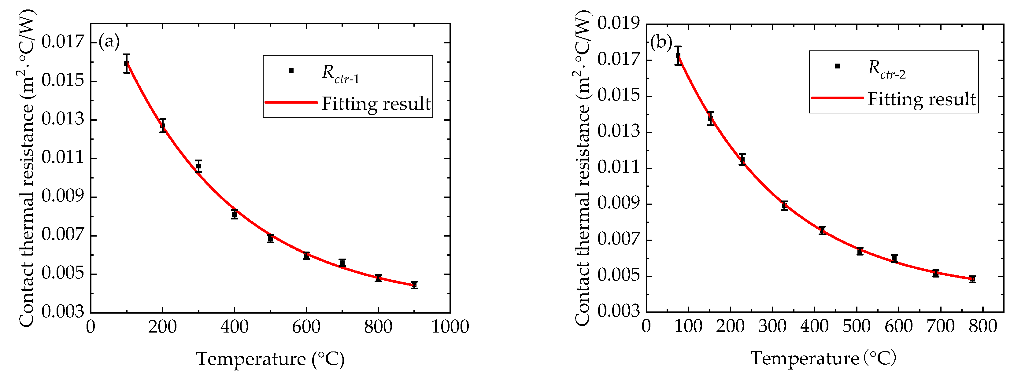
3.1. Calibration Method of Contact Thermal Resistance

Contact thermal resistance is mainly affected by surface geometry, pressure load, temperature, and contact material. In the calibration process, factors other than temperature should be avoided as far as possible. In this paper, 304L stainless steel was used as the calibration material of contact thermal resistance. The geometrical morphology of the material is represented by its surface roughness, so the 304L stainless steel with the same surface processing type as the full-scale container was selected to reduce the influence of roughness. In addition, the contact material is always an SiC plate and 304L stainless steel, so this factor can be ignored. Therefore, the function relationship between temperature and contact thermal resistance needs to be calibrated under the same pressure loaded on the specimen.

In order to obtain the temperature gradient across the 304L stainless steel, three thermocouples sheathed with stainless steel of 2 mm in diameter, were placed in the holes drilled to the center of the specimen at distances of 10 mm, 25 mm, and 40 mm from the heating plate. The locations of the thermocouples are shown in Figure 4.

In a previous study [27], the sensitivities of both heat flux sensors installed on the plates were calibrated with varying temperatures, as shown in Equation (16) and Equation (17). Thus, the heat flux across the calibration material can be calculated by Equation (18), in which E₁ and E₂ represent the output voltage of two heat flux sensors, respectively.

$$S_{down}(T_{down})=2.82\times {10}^{-3}\times T_{down}+48.25$$

(16)

$$S_{up}(T_{up})=2.59\times {10}^{-3}\times T_{up}+48.93$$

(17)

$$q=\frac{S_{up}\left(T_{up}\right)\times E_{up}+S_{down}\left(T_{down}\right)\times E_{down}}{2}$$

(18)

The measurement results for when the heating temperature was 100 °C are shown in Figure 5; here, Figure 5a gives the two heat flux testing results, and Figure 5b shows the linearity of the temperature gradient in the material. According to the least square method, the temperature value of the hot end (T_H) was 89.3 °C, while the cold end (T_C) of the calibration material was 87.1 °C. The average heat flux across the specimen was 672.03 W/m², which was calculated by Equation (18).

Therefore, the contact thermal resistances of both plates are expressed by Equation (19) and Equation (20).

$$R_{ctr-down}\left(T_{down}\right)=\frac{T_{down}-T_H}{q}$$

(19)

$$R_{ctr-up}\left(T_{up}\right)=\frac{T_C-T_{up}}{q}$$

(20)

In order to study the relationship between contact thermal resistance and temperature (as well as for future research), the setting temperature range of the calibration experiment was from 100 to 900 °C for every 100 °C, and the values of contact thermal resistance at other temperatures were deduced. Figure 6 shows the calibration results of contact thermal resistance at different heating temperatures. It can be seen that there were non-linear exponential relationships between the contact thermal resistances of both plates and temperature. With the increase of temperature, the contact thermal resistance between the two plates and the calibration material decreased gradually. Due to the expansion of the calibration material, the actual contact area between the two plates increased. The contact thermal resistance fitting results of both plates are shown in Equation (21) and Equation (22).

$$R_{ctr-down}\left(T_{down}\right)=0.00334+0.01722\times e^{-\frac{T_{down}}{325.68973}}$$

(21)

$$R_{ctr-up}\left(T_{up}\right)=0.00392+0.01776\times e^{-\frac{T_{up}}{262.50754}}$$

(22)

Therefore, during the experimental test, the contact thermal resistance between the PCM specimen in a container and the plates could be estimated approximately under the same pressure by using Equation (21) and Equation (22).

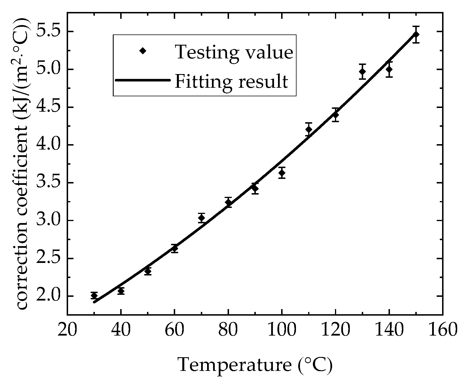
3.2. Calibration Method of Calorific Absorption Correction Coefficient of Heat Flux Sensor

In the measurement of heat of absorption, the correction coefficient related to the heat flux sensor needs to be calibrated. The 304L stainless steel was also used as the calibration material, and its volume specific heat value varying with temperature (C_V-304 (T)) was measured by a HotDisk analyzer. The relationship between the volume specific heat and temperature is expressed in Equation (23).

$$C_{V-304L}(T)=3.8254+0.0014\times T$$

(23)

In each temperature step, the correction coefficient is considered to be linear. When the temperature is changed from T_a to T_b, the change of areal enthalpy h_A (T_a, T_b) can be expressed as h_A (T_mean). Based on Equations (8)–(11), the correction coefficient S_HFM (T_mean) can be calculated by Equation (24) at each mean calibration temperature, which represents the heat stored by the heat flux sensors within the temperature step from T_a to T_b.

$$S_{HFM}(T_{mean})=\frac{h_A-C_{V-304L}(T_{mean})\times {\delta }_{304L}\times \Delta T}{\Delta T}$$

(24)

During the calibration process, the initial temperature of both heating plates was set to 25 °C, and the temperature step was 10 °C. The calibration average temperature range was from 30 to 150 °C. Equation (24) was used for every temperature step to calculate the correction coefficient at its mean temperature. After the calibration process was finished, the calibration results were fitted to obtain the function of the correction coefficient varying with the average temperature. The fitting function is shown in Equation (25), and the fitting curve is shown in Figure 7.

$$S_{HFM}\left(T_{mean}\right)=1.2971+0.0190\times T_{mean}+5.9365\times {10}^{-5}\times T_{mean}^2$$

(25)

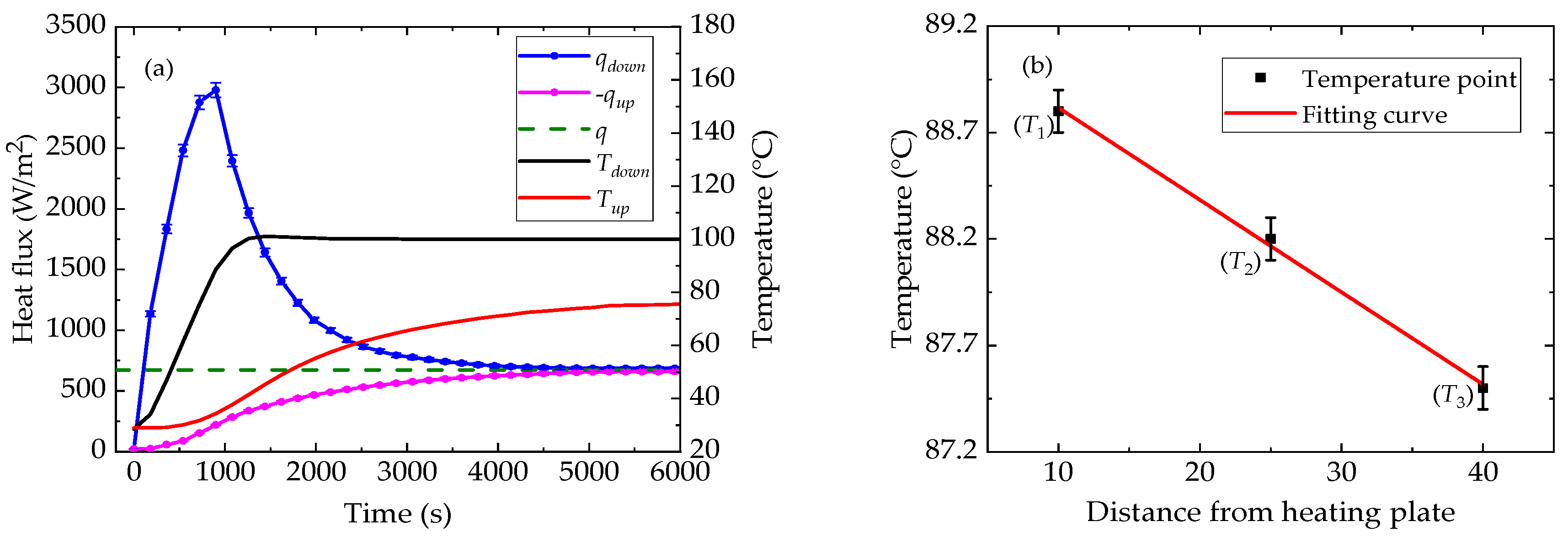
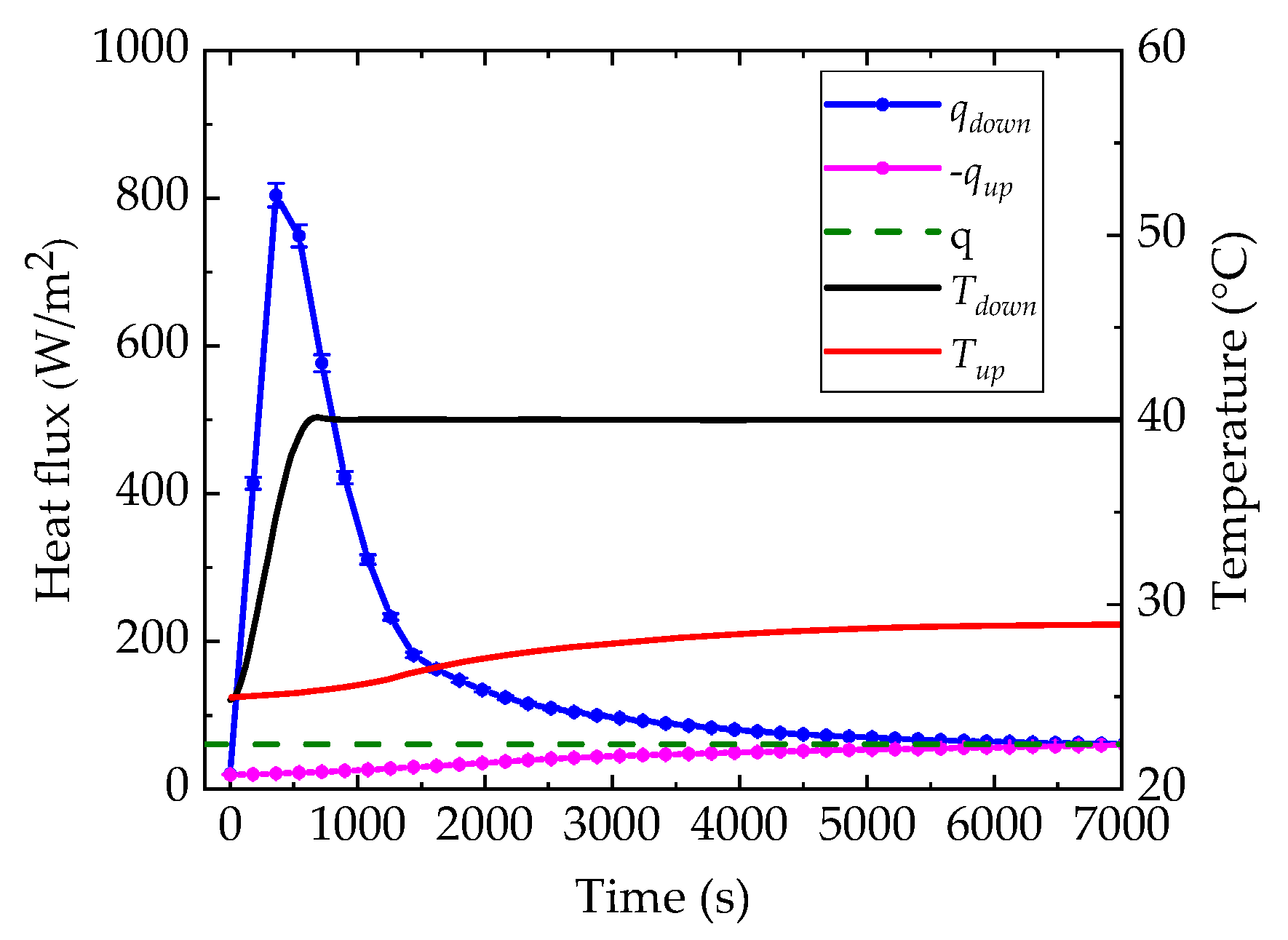
4. Experimental Results

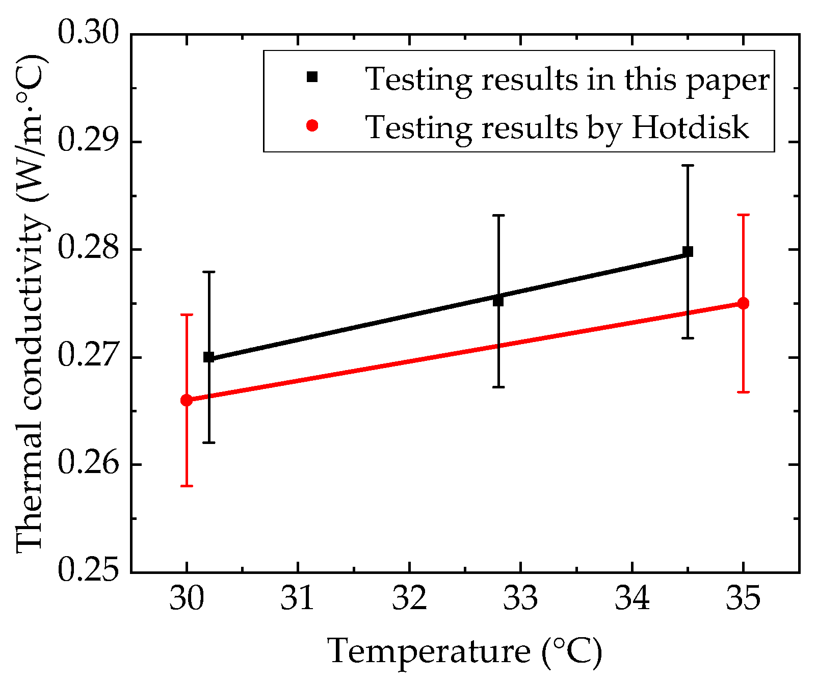
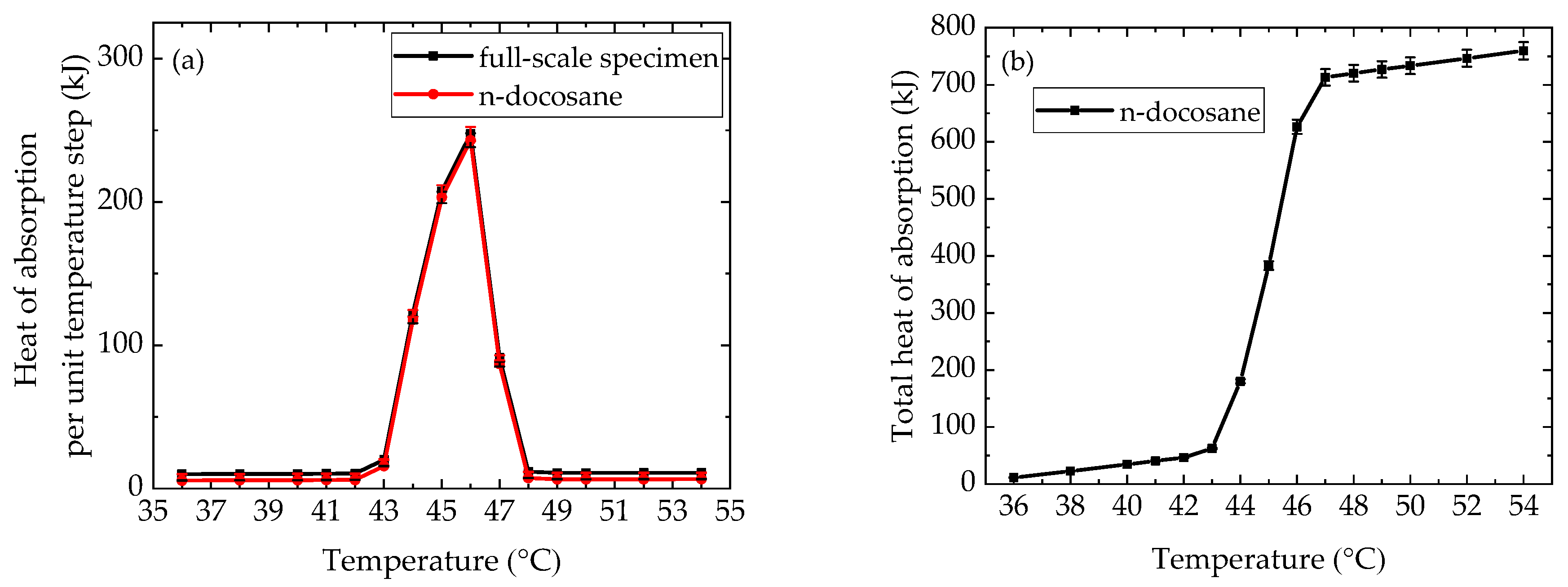
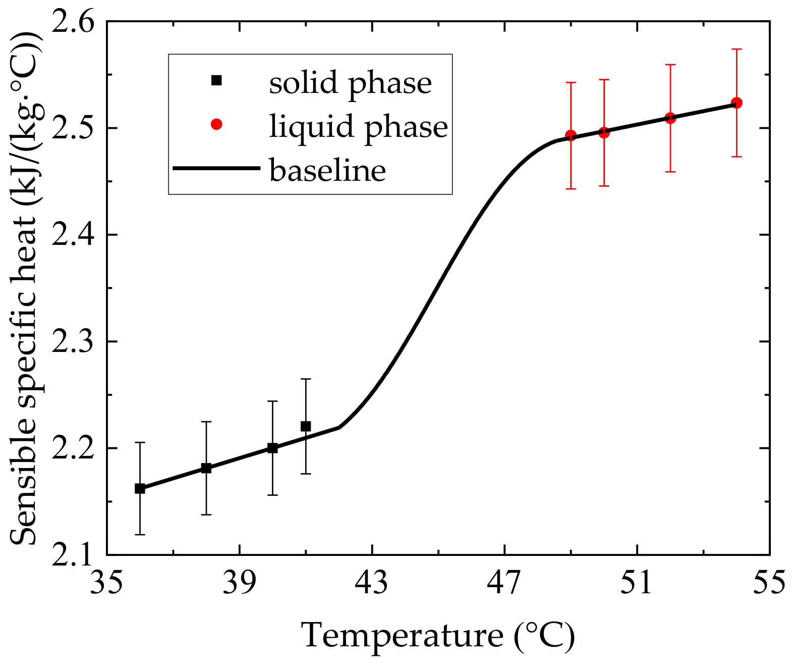
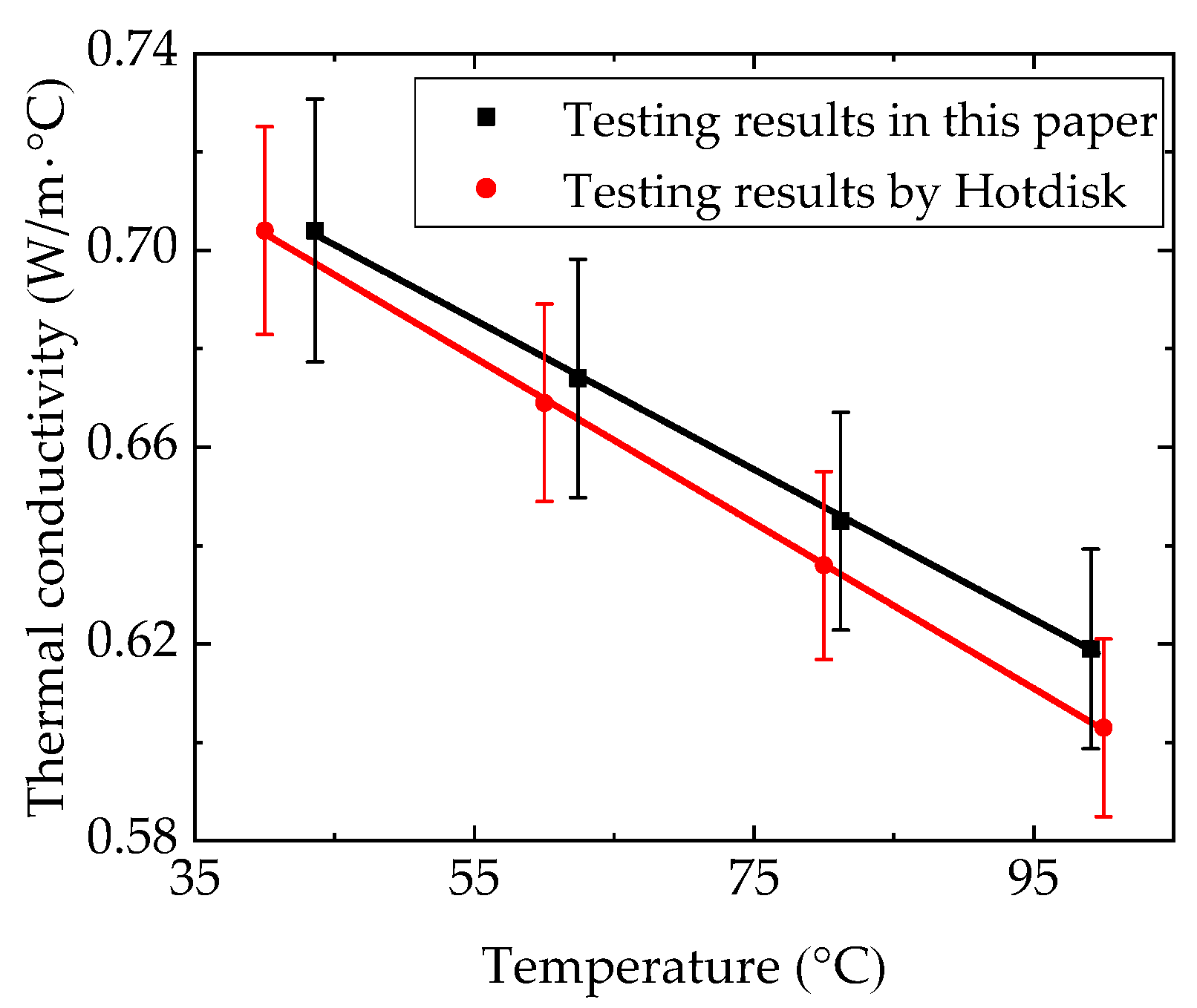
4.1. Thermophysical Properties of n-docosane in the Container

The thermophysical properties of n-docosane in the container include the thermal conductivity of the solid phase, the heat of absorption, and the phase change temperature range. In order to verify the measurement result of the heat of absorption, the latent heat of n-docosane was also calculated to compare with the DSC results.

At the beginning, the n-docosane with 8.8 mg was tested by DSC to provide a reference for the full-scale measurement. The results of DSC show that the initial phase change temperature of n-docosane was 42.9 °C and the latent heat was 256.9 J/g.

Based on the DSC results, n-docosane is a solid specimen when the temperature is below 40 °C. Thus, the temperature of one plate was set to 40 °C, and the other plate was regarded as the cold plate in order to measure the thermal conductivity. Figure 8 shows the curves of the testing results of heat fluxes and temperatures. It shows that the temperatures on both plates were 40.0 °C and 28.9 °C, respectively. Besides, the average heat flux across the specimen was 60.92 W/m².

Based on the testing results, the values of contact thermal resistances were calculated by Equation (21) and Equation (22). The results show that the contact thermal resistances at both ends of the full-scale specimen were 0.0186 m²·°C/W and 0.0198 m²·°C/W, respectively. Then, the thermal resistance of n-docosane inside the full-scale specimen was 0.1431 m²·°C/W, which was calculated using Equation (6). Therefore, the thermal conductivity of n-docosane was 0.280 W/m·°C, with a mean temperature 34.5 °C. If the contact thermal resistance is not taken into consideration, the testing result would be 0.221 W/m·°C, with a mean temperature of 34.4 °C. In order to verify the accuracy of the measurement result, a HotDisk analyzer was used to measure the thermal conductivity at 35.0 °C. The measurement result was 0.275 W/m·°C. It can be calculated that the deviation was 19.6% without considering the contact thermal resistance, while the deviation was 1.8% when the contact thermal resistance was taken into consideration. In order to obtain the function of thermal conductivities of n-docosane varying with temperatures, the heating temperatures were set to 38 °C and 35 °C using the same method, so the mean temperatures of the specimen were 32.8 °C and 30.2 °C, respectively. In addition, the HotDisk analyzer was used to measure thermal conductivity at 30 °C for comparison. Figure 9 gives the thermal conductivities of n-docosane by using the method in this paper and HotDisk analyzer at different temperatures.

Therefore, the fitting result of solid thermal conductivity of n-docosane measured in this paper is expressed in Equation (26). It can be calculated that the thermal conductivity of n-docosane at 25 °C was 0.258 W/m·°C. Some references show that the thermal conductivity of n-docosane ranges from 0.22 to 0.26 W/m·°C at room temperature [7,28,29]. Moreover, Rao et al. [30] noticed that the thermal conductivity of n-docosane increases when the temperature increases. Therefore, the measurement results are reliable.

$${\lambda }_{C22}=0.00226\times T+0.20168$$

(26)

Then, the total heat of absorption, the phase change temperature range, and the latent heat were measured by the DHFMA method. The mass of n-docosane in the container was 2.614 kg. Figure 10 gives the curves of temperature step and heat flux values of both heat flux sensors in order to measure the heat of absorption of n-docosane from 42.0 to 43.0 °C; Figure 10a refers to the lower heating plate, while Figure 10b refers to the upper heating plate. The areal enthalpy of the specimen at the temperature step can be calculated by the area enclosed by the heat flux curve and q_equi. Similarly, other temperature step measurement results can be obtained.

According to Equations (9)–(14), the results of heat of absorption for full-scale specimen and n-docosane at each temperature step can be calculated, as shown in Figure 11, in which (a) presents the heat of absorption per unit temperature step for both full-scale specimen and n-docosane, and (b) presents the accumulated total heat of absorption for n-docosane. It can be found that the temperature step was 2 °C when the temperature was under 40 °C and above 50 °C, while the temperature step was 1 °C between 40 and 50 °C. The design of this temperature step is intended to not only accurately measure the phase change temperature range but to also effectively save testing time.

Figure 11 clearly shows that the full-scale specimen has a distinct endothermic zone in the test temperature interval, which is due to the large amount heat of absorption by phase change of n-docosane inside the full-scale specimen. In addition, when the temperature changes from 42 to 43 °C, the heat of absorption curve begins to deviate and the phase change of n-docosane begins. The initial temperature point of phase change refers to the mean temperature 42.5 °C. Similarly, the end temperature point of phase change refers to 48.5 °C.

In addition, due to the mass of n-docosane being 2.614 kg, the specific heat values of solid and liquid phases are calculated by Equation (14). Figure 12 gives the sensible specific heat value of n-docosane. Then, test results were fit to obtain the baseline, which refers to the sensible specific heat value. Based on the results of Figure 11, it can be concluded that the total enthalpy of n-docosane in the phase change range (42–49 °C) was 259.92 kJ/kg. The sensible specific heat in the phase change range can be obtained from Figure 12. As such, the total sensible enthalpy, which was 16.46 kJ/kg, was calculated by the area enclosed by the sensible specific heat from 42 to 49 °C. Therefore, the latent enthalpy of n-docosane was 243.46 kJ/kg. Compared with the published data [7,28,29,30,31] in which the initial phase change temperature of n-docosane was from 40.67 to 43.15 °C, and the latent heat is from 194.6 to 241.3 kJ/kg, the measurement results in this paper are reasonable.

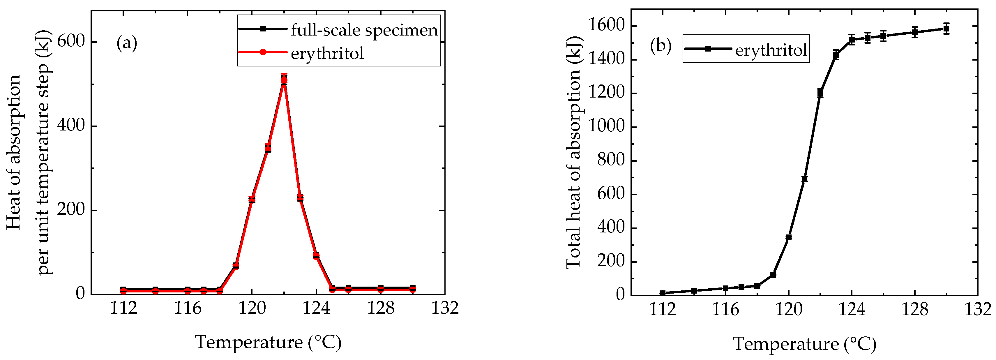
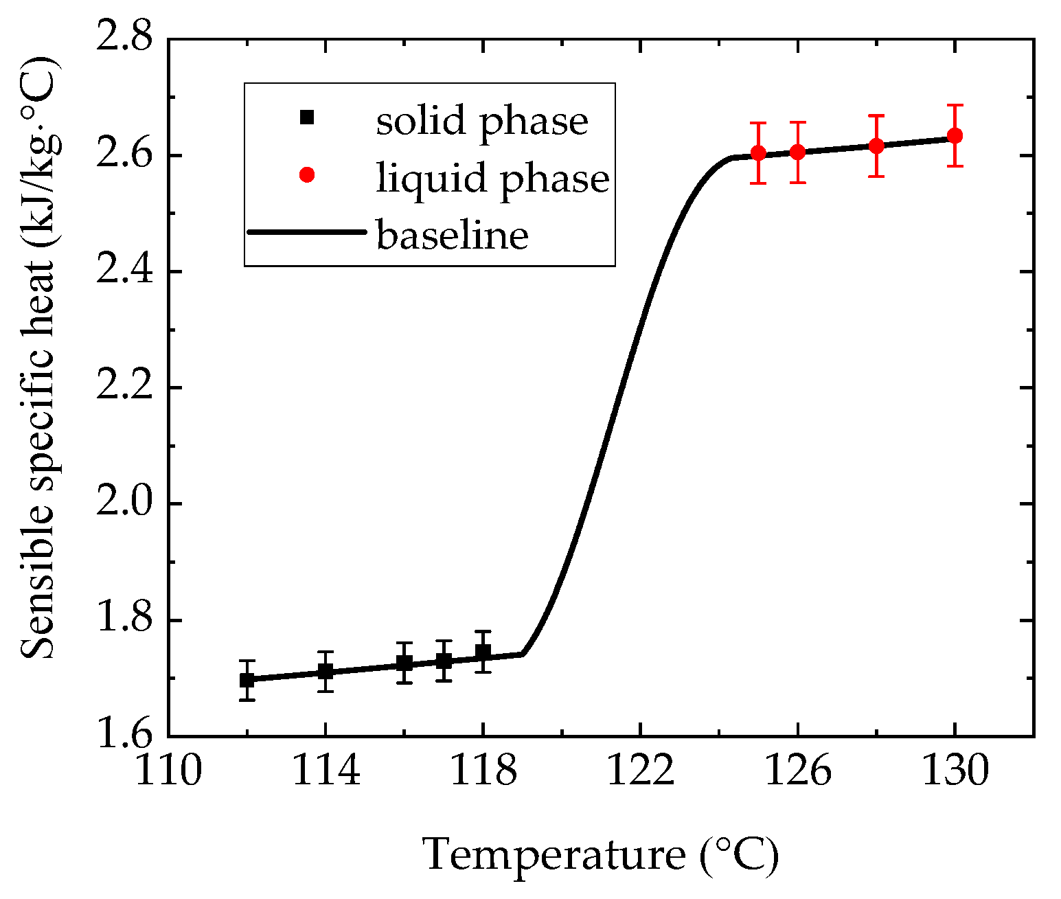
4.2. Thermophysical Properties of Erythritol in the Container

The thermal conductivities of erythritol are measured at four heating temperatures, 50 °C, 70 °C, 90 °C, and 110 °C, in which the mean temperatures of erythritol in the container are 43.6 °C, 62.4 °C, 81.2 °C, and 99.6 °C. During the measurement, the influence of contact thermal resistance was taken into consideration for each test. For comparison, the thermal conductivities of erythritol were measured by a HotDisk analyzer whose sensor was located in the furnace, where the temperatures were set as 40.0 °C, 60.0 °C, 80.0 °C, and 100.0 °C. The thermal conductivities of erythritol at different temperatures were measured through an experimental process which is similar to the measurement process of n-docosane, and the results are shown in Figure 13.

It can be seen that the solid thermal conductivity of erythritol decreased while the temperature increased. The maximum deviation between the measurement results, considering contact thermal resistance, and those of a HotDisk analyzer was 2.6%. The fitting result of solid thermal conductivity of erythritol measured in this paper is expressed in Equation (27).

$${\lambda }_{ery}=-0.00152\times T+0.76952$$

(27)

Compared with the published data in which the thermal conductivity of erythritol at room temperature was from 0.710 to 0.733 W/m·°C [32,33,34], the result calculated by Equation (27) was 0.731 W/m·°C at the temperature of 25 °C. Therefore, the testing results are accurate at different temperatures by considering the contact thermal resistance.

Figure 14 gives the testing results for heat of absorption of full-scale specimen with erythritol, in which (a) presents the heat of absorption per unit temperature step and (b) presents the accumulated total heat of absorption. The mass of n-docosane in the container was 4.225 kg.

It can be seen that there is also an obvious zone which indicating the heat of absorption in the full-scale specimen. In this temperature range, the solid–liquid phase change of erythritol occurred inside the full-scale specimen, which absorbed a large amount of heat. When the temperature rose from 118.0 to 119.0 °C, the curve of heat of absorption deflected obviously. Thus, the initial temperature point of phase change refers to the mean temperature 118.5 °C. Similarly, the end temperature point of phase change refers to 124.5 °C. It can be concluded that the phase change temperature range of erythritol was from 118.5 to 124.5 °C.

Figure 15 gives the sensible specific heat value of erythritol, with reference to the baseline. It can be concluded that the total enthalpy of erythritol in the phase change range was 345.78 kJ/kg, including the sensible enthalpy and the latent enthalpy. Based on the curve of sensible specific heat shown in Figure 15, the area from 118 to 125 °C was 13.94 kJ/kg, which can be considered the sensible enthalpy value of erythritol. Therefore, the latent enthalpy of erythritol was 331.84 kJ/kg. Compared with the published data [35,36,37], in which the initial phase change temperature of erythritol was from 117.0 to 119.3 °C and the latent heat was from 315 to 344 kJ/kg. Besides, the latent enthalpy measured by DSC was 344.6 J/g. Therefore, the measurement results in this paper are reasonable.

4.3. Uncertainty Analysis

Uncertainty analyses include the uncertainty analysis of the thermal conductivity measurement and the uncertainty analysis of the heat of absorption measurement.

Based on Equations (1)–(7), the thermal resistance and thermal conductivity of the PCM in the container can be arranged as Equation (27) and Equation (28). Therefore, the uncertainty sources of the thermal conductivity measurement include uncertainties of temperature difference, thickness, heat flow, the thermal conductivity of the container measured by a HotDisk analyzer, and the contact thermal resistance calibration.

$$R_{PCM}=R-R_{ctr-down}-R_{ctr-up}-R_{box-down}-R_{box-up}=\frac{\Delta T}{q}-R_{ctr}-\frac{{\delta }_{box}}{{\lambda }_{box}}$$

(28)

$${\lambda }_{PCM}=\frac{{\delta }_{PCM}}{R_{PCM}}$$

(29)

Uncertainty analysis was performed using the thermal conductivity test data of erythritol in a container with the heating temperature of 110 °C. Firstly, the temperature difference was calculated by the temperatures measured on the two plates. By considering the uncertainty of the temperature difference measurement and the acquisition error of data acquisition card [38], the standard uncertainty of temperature difference measurement was 0.11 °C. Then, the thickness of the container was measured by a vernier caliper, and the thermal expansion was also taken into consideration. The thermal expansion coefficient was measured by DIL 402C which is purchase from NETZSCH (Shanghai) Machinery and Instruments Co. Ltd. Branch Office Liaoning (Shenyang, Liaoning, China). As such, the standard uncertainty of the thickness measurement was 9.69 × 10⁻⁶ m. Furthermore, the uncertainty of the heat flow measurement comes from the calibration process of the heat flux meter. Sources of calibration uncertainty include the uncertainty of thermal conductivity measured by a HotDisk analyzer, the uncertainty of the temperature difference measurement, and the uncertainty of the thickness measurement. The standard uncertainty of the heat flow measurement was 4.45 W/m². Similarly, the standard uncertainty of thermal contact resistance calibration was 6.82 × 10⁻⁶ m²·°C/W. Equation (30) gives the uncertainty composition formula of PCM thermal resistance, and Equation (31) refers to the standard uncertainty of thermal conductivity of a PCM.

$$u_{R_{PCM}}=\sqrt{{\left(\frac{\partial R_{PCM}}{\partial \Delta T}\times u_{\Delta T}\right)}^2+{\left(\frac{\partial R_{PCM}}{\partial q}\times u_q\right)}^2+{\left(\frac{\partial R_{PCM}}{\partial R_{ctr}}\times u_{R_{ctr}}\right)}^2+{\left(\frac{\partial R_{PCM}}{\partial {\delta }_{box}}\times u_{{\delta }_{box}}\right)}^2+{\left(\frac{\partial R_{PCM}}{\partial {\lambda }_{box}}\times u_{{\lambda }_{box}}\right)}^2}$$

(30)

$$u_{{\lambda }_{PCM}}=\sqrt{{\left(\frac{\partial {\lambda }_{PCM}}{\partial {\delta }_{PCM}}\times u_{{\delta }_{PCM}}\right)}^2+{\left(\frac{\partial {\lambda }_{PCM}}{\partial R_{PCM}}\times u_{R_{PCM}}\right)}^2}$$

(31)

Therefore, the standard uncertainty of the thermal conductivity measurement of erythritol was 2.03 × 10⁻² W/m·°C when the heating temperature was 110 °C, and the relative standard uncertainty was 3.27%. In this way, the uncertainty of the thermal conductivity measurement of n-docosane and erythritol in the container at different heating temperature can be obtained. The results show that the relative standard uncertainty was better than 3.79%.

In addition, Equation (32) gives the calculate formula for heat of absorption of the PCM in the container, so the sources of uncertainty in the calculation of the heat of absorption can be obtained.

$$Q_{PCM}=\frac{h_{As}}{\delta }\times V_s-C_{box}\times V_{box}$$

(32)

Uncertainty analysis was performed using the heat of absorption test data of erythritol in a container with temperature step from 120 to 121 °C. Equation (33) gives the uncertainty composition formula for each temperature step.

$$u_{Q_{PCM}}=\sqrt{{\left(\frac{\partial Q_{PCM}}{\partial h_s}\times u_{h_{As}}\right)}^2+{\left(\frac{\partial Q_{PCM}}{\partial \delta }\times u_{\delta }\right)}^2+{\left(\frac{\partial Q_{PCM}}{\partial V_s}\times u_{Vs}\right)}^2+{\left(\frac{\partial Q_{PCM}}{\partial C_{box}}\times u_{Cbox}\right)}^2+{\left(\frac{\partial Q_{pcm}}{\partial V_{box}}\times u_{Vbox}\right)}^2}$$

(33)

The uncertainty of areal enthalpy depends on the uncertainty of the heat flow measurement, which was 1.99%. In this temperature step, h_As = 3.90 × 10³ kJ/m². As such, the standard uncertainty of h_As (u_hAs) was 77.61 kJ/m². The standard uncertainty sources of thickness measurements include vernier caliper measurement uncertainty, specimen thermal expansion uncertainty, and thermal expansion measurement uncertainty. Thus, the standard uncertainty of δ (u_δ) was 9.69 × 10⁻⁶ m. The volume uncertainty depends on the uncertainty of the thickness measurement. As such, it can be calculated that the standard uncertainties of the specimen (u_Vs) and the container (u_Vbox) were 1.16 × 10⁻⁶ m³ and 1.56 × 10⁻⁶ m³, respectively. Furthermore, the volume specific heat of the container was measured by a HotDisk analyzer. The measurement accuracy of C_v-304 was 7%, which was subject to uniform distribution. Meanwhile, C_v-304 = 3.99 kJ/m³ in this temperature step, so the standard uncertainty of C_v-304 is 3.99 × (7%/$\sqrt{3}$) = 0.16 kJ/m³. In addition, δ = 0.05 m, V_s = 4.50 × 10⁻³ m³, and V_box = 1.14 × 10⁻³ m³. By substituting all the parameters into Equation (33), it can be calculated that the standard uncertainty of Q_PCM (u_QPCM) was 6.99 kJ. As shown in Figure 14, the heat of absorption from 120 to 121 °C was Q_PCM = 3.51 × 10² kJ. Therefore, the relative standard uncertainty can be calculated in Equation (34). It can be concluded that the relative standard uncertainty mainly depends on the uncertainty of the heat flow measurement.

$${u^{\prime }}_{Q_{PCM}}=\frac{u_{Q_{PCM}}}{Q_{PCM}}\times 100\%=1.99\%$$

(34)

5. Conclusions

In this paper, a method to measure the thermophysical parameters of a PCM inside a full-scale specimen was proposed. The thermophysical parameters included solid thermal conductivity, phase change temperature range, and heat of absorption. Calibration methods for the heat of absorption correction coefficient and the contact thermal resistance between the specimen and plates were proposed. Furthermore, in order to obtain the thermal conductivity and heat of absorption of a PCM inside a full-scale specimen, calculation methods were deduced. During the experiment, n-docosane and erythritol in the full-scale 304L stainless steel container were selected as the PCMs. Their thermophysical properties were tested by the method presented in this paper. It can be found that the test results in this paper were in good agreement with the HotDisk analyzer results and the published data; the uncertainty analysis indicated that the relative standard uncertainty for thermal conductivity of the PCM in the container was better than 3.79%, and the relative standard uncertainty for heat of absorption in each temperature step was 1.99%. Therefore, the test methods for measuring thermophysical properties of a PCM inside a full-scale specimen proposed in this paper are accurate and reasonable.

References

1. Xie, N.; Huang, Z.W.; Luo, Z.G.; Gao, X.N.; Fang, Y.T.; Zhang, Z.G. Inorganic salt hydrate for thermal energy storage. Appl. Sci. 2017, 7, 1317. [Google Scholar] [CrossRef]
2. Mahavar, S.; Sengar, N.; Rajawat, P.; Verma, M.; Dashora, P. Design development and performance studies of a novel single family solar cooker. Renew. Energy 2012, 47, 67–76. [Google Scholar] [CrossRef]
3. Hasan, A.; Hejase, H.; Abdelbaqi, S.; Assi, A.; Hamdan, M.O. Comparative effectiveness of different phase change materials to improve cooling performance of heat sinks for electronic devices. Appl. Sci. 2016, 6, 226. [Google Scholar] [CrossRef]
4. Sqanson, T.D.; Birur, G.C. NASA thermal control technologies for robotic spacecraft. Appl. Therm. Energy 2003, 23, 1055–1065. [Google Scholar] [CrossRef] [Green Version]
5. Renteria, J.D.; Nika, D.L.; Balandin, A.A. Graphene thermal properties: Applications in thermal management and energy storage. Appl. Sci. 2014, 4, 525–547. [Google Scholar] [CrossRef]
6. Frusteri, F.; Leonardi, V.; Vasta, S.; Restrccia, G. Thermal conductivity measurement of a PCM based storage system containing carbon fibers. Appl. Therm. Energ. 2005, 25, 1623–1633. [Google Scholar] [CrossRef]
7. Sari, A.; Karaipekli, A. Thermal conductivity and latent heat thermal energy storage characteristics of paraffin/expanded graphite composite as phase change material. Appl. Therm. Energy 2007, 27, 1271–1277. [Google Scholar] [CrossRef]
8. Xiao, X.; Zhang, P.; Li, M. Thermal characterization of nitrates and nitrates/expanded graphite mixture phase change materials for solar energy storage. Energ. Convers. Manag. 2013, 73, 86–94. [Google Scholar] [CrossRef]
9. Wang, W.L.; Yang, X.X.; Fang, Y.T.; Ding, J.; Yan, J.Y. Enhanced thermal conductivity and thermal performance of form-stable composite phase change materials by using beta-Aluminum nitride. Appl. Energy 2009, 86, 1196–1200. [Google Scholar] [CrossRef]
10. Chen, M.Z.; Wan, L.; Lin, J.T. Effect of phase-change materials on thermal and mechanical properties of asphalt mixtures. J. Test Eval. 2012, 40, 746–753. [Google Scholar] [CrossRef]
11. Motahar, S.; Nikkam, N.; Alemrajabi, A.A.; Khodabandeh, R.; Toprak, M.S.; Muhammed, M. Experimental investigation on thermal and rheological properties of n-octadecane with dispersed TiO2 nanoparticles. Int. Commun. Heat. Mass. 2014, 56, 114–120. [Google Scholar] [CrossRef]
12. Xiao, X.; Zhang, P.; Li, M. Effective thermal conductivity of open-cell metal foams impregnated with pure paraffin for latent heat storage. Int. J. Therm. Sci. 2014, 81, 94–105. [Google Scholar] [CrossRef]
13. Aktay, K.S.D.C.; Tamme, R.; Muller-Steinhagen, H. Thermal conductivity of high-temperature multicomponent materials with phase change. Int. J. Thermophys. 2008, 29, 678–692. [Google Scholar] [CrossRef]
14. Wang, X.; Yu, H.; Li, L.; Zhao, M. Research on temperature dependent effective thermal conductivity of composite-phase change materials (PCMs) wall based on steady-state method in a thermal chamber. Energy Build. 2016, 126, 408–414. [Google Scholar] [CrossRef]
15. Abyzov, A.M.; Shakhov, F.M. Measurement of the effective thermal conductivity of particulate materials by the steady-state heat flow method in a cuvette. Meas. Sci. Technol. 2014, 25, 125009. [Google Scholar] [CrossRef]
16. Stacey, C.; Simplin, A.J.; Jarrett, R.N. Techniques for reducing thermal contact resistance in steady-state thermal conductivity measurements on polymer composites. Int. J. Thermophys. 2016, 37, 107. [Google Scholar] [CrossRef]
17. Sun, X.Q.; Lee, K.O.; Medina, M.A.; Chu, Y.H.; Li, C.C. Melting temperature and enthalpy variations of phase change materials (PCMs): A differential scanning calorimetry (DSC) analysis. Phase Transit. 2018, 91, 667–680. [Google Scholar] [CrossRef]
18. Jiang, Y.F.; Sun, Y.P.; Liu, M. Eutectic Na2CO3-NaCl salt: A new phase change material for high temperature thermal storage. Sol. Energy Mat. Sol. C 2016, 152, 155–160. [Google Scholar] [CrossRef]
19. Banu, D.; Feldman, D.; Hawes, D. Evaluation of thermal storage as latent heat in phase change material wallboard by differential scanning calorimetry and large scale thermal testing. Thermochim. Acta 1998, 317, 39–45. [Google Scholar] [CrossRef]
20. Zhang, Y.P.; Jiang, Y.; Jiang, Y. A simple method, the T-history method, of determining the heat of fusion, specific heat and thermal conductivity of phase-change materials. Meas. Sci. Technol. 1999, 10, 201–205. [Google Scholar]
21. Peck, J.H.; Kim, J.J.; Kang, C.D.; Hong, H.K. A study of accurate latent heat measurement for a PCM with a low melting temperature using T-history method. Int. J. Refrig. 2006, 29, 1225–1232. [Google Scholar] [CrossRef]
22. Lázaro, A.; Günther, E.; Mehling, H.; Hiebler, S.; Marin, J.M.; Zalba, B. Verification of a T-history installation to measure enthalpy versus temperature curves of phase change materials. Meas. Sci. Technol. 2006, 17, 2168–2174. [Google Scholar] [CrossRef]
23. Kravvaritis, E.D.; Antonopoulos, K.A.; Tzivanidis, C. Improvements to the measurement of the thermal properties of phase change materials. Meas. Sci. Technol. 2010, 21, 045103. [Google Scholar] [CrossRef]
24. Shukla, N.; Fallahi, A.; Kosny, J. Performance characterization of PCM impregnated gypsum board for building applications. Energy Procedia 2012, 30, 370–379. [Google Scholar] [CrossRef]
25. Kosny, J.; Kossecka, E.; Brzezinski, A.; Tleoubaev, A.; Yarbrough, D. Dynamic thermal performance analysis of fiber insulations containing bio-based phase change materials (PCMs). Energy Build. 2012, 52, 122–131. [Google Scholar] [CrossRef]
26. Biswas, K.; Shukla, Y.; Desjarlais, A.; Rawal, R. Thermal characterization of full-scale PCM products and numerical simulations, including hysteresis, to evaluate energy impacts in an envelope application. Appl. Therm. Energy 2018, 138, 501–512. [Google Scholar] [CrossRef]
27. Wang, Y.; Xiao, P.; Dai, J.M. Design and construction of a new steady-state apparatus for medium thermal conductivity measurement at high temperature. Rev. Sci. Instrum. 2017, 88, 104903. [Google Scholar] [CrossRef]
28. Chang, S.J.; Wi, S.; Lee, J.; Kim, S. Thermal performance analysis of phase change materials composed of double layers considering heating and cooling period. J. Ind. Eng. Chem. 2019, 72, 255–264. [Google Scholar] [CrossRef]
29. Li, J.F.; Lu, W.; Zeng, Y.B.; Luo, Z.P. Simultaneous enhancement of latent heat and thermal conductivity of docosane-based phase change material in the presence of spongy grapheme. Sol. Energy Mat. Sol. C 2014, 128, 48–51. [Google Scholar] [CrossRef]
30. Rao, Z.H.; Wang, S.F.; Zhang, Y.L.; Peng, F.F.; Cai, S.H. Molecular dynamics simulation of the thermophysical properties of phase change material. Acta. Phys. Sin. 2013, 62, 056601. [Google Scholar]
31. Hearn, J.D.; Smith, G.D. Ozonolysis of mixed oleic acid/n-docosane particles: The roles of phase, morphology, and metastable states. J. Phys. Chem. A 2007, 111, 11059–11065. [Google Scholar] [CrossRef] [PubMed]
32. Oya, T.; Nomura, T.; Tsubotga, M.; Okinaka, N. Thermal conductivity enhancement of erythritol as PCM by using graphite and nickel particles. Appl. Therm. Energy 2013, 61, 825–828. [Google Scholar] [CrossRef]
33. Lee, S.Y.; Shin, H.K.; Park, M.; Rhee, K.Y.; Park, S.J. Thermal characterization of erythritol/expanded graphite composites for high thermal storage capacity. Carbon 2014, 68, 67–72. [Google Scholar] [CrossRef]
34. Karthik, M.; Faik, A.; Blanco-Rodríguez, P.; Rodríguez-Aseguinolaza, J.; D’Aguanno, B. Preparation of erythritol–graphite foam phase change composite with enhanced thermal conductivity for thermal energy storage applications. Carbon 2015, 94, 266–276. [Google Scholar] [CrossRef]
35. Talja, R.A.; Roos, Y.H. Phase and state transition effects on dielectric, mechanical, and thermal properties of polyols. Thermochim. Acta 2001, 380, 109–121. [Google Scholar] [CrossRef]
36. Kholmanov, I.; Kim, J.; Ou, E.; Ruoff, R.S.; Shi, L. Continuous carbon nonatube-ultrathin graphite hybrid foams for increased thermal conductivity and suppressed subcooling in composite phase change materials. ACS Nano 2015, 9, 11699–11707. [Google Scholar] [CrossRef] [PubMed]
37. Diarce, G.; Gandarias, I.; Campos-Celador, Á.; Garcia-Romero, A.; Griesser, U.J. Eutectic mixtures of sugar alcohols for thermal energy storage in the 50–90 °C temperature range. Sol. Energy Mat. Sol. C 2015, 134, 215–226. [Google Scholar] [CrossRef]
38. Jensen, C.; Xing, C.; Folsom, C.; Ban, H.; Phillips, J. Design and validation of a high-temperature comparative thermal-conductivity measurement system. Int. J. Thermophys. 2012, 33, 311–329. [Google Scholar] [CrossRef]
Figure 1. Structure of the measurement apparatus. (a) Diagrammatic sketch, (b) photograph, and (c) heating plate.
Applsci 09 02422 g001
Figure 2. The 3D diagram and cross section of the testing specimen.
Applsci 09 02422 g002
Figure 3. Schematic diagram of steady-state thermal resistance series structure.
Applsci 09 02422 g003
Figure 4. The location of the thermocouples in the specimen.
Applsci 09 02422 g004
Figure 5. Results of heat fluxes and temperatures in the calibration when the heating temperature was 100 °C. (a) Curves of heat flux and temperature measurements. (b) Temperature gradient in the material.
Applsci 09 02422 g005
Figure 6. The calibration results of contact thermal resistance at different heating temperatures. (a) Hot plate. (b) Cold plate.
Applsci 09 02422 g006
Figure 7. The fitting curve of correction coefficient varying with temperature.
Applsci 09 02422 g007
Figure 8. The curves of testing results of heat fluxes and temperatures.
Applsci 09 02422 g008
Figure 9. Thermal conductivities of n-docosane at different temperatures.
Applsci 09 02422 g009
Figure 10. Curves of temperature step and heat flow values on both plates. (a) Bottom plate. (b) Top plate.
Applsci 09 02422 g010
Figure 11. Testing results for heat of absorption of full-scale specimen and n-docosane. (a) Heat of absorption per unit temperature step. (b) Total heat of absorption.
Applsci 09 02422 g011
Figure 12. Sensible specific heat value of n-docosane.
Applsci 09 02422 g012
Figure 13. Thermal conductivities of erythritol at different temperatures.
Applsci 09 02422 g013
Figure 14. Testing results for heat of absorption of full-scale specimen and erythritol. (a) Heat of absorption per unit temperature step. (b) Total heat of absorption.
Applsci 09 02422 g014
Figure 15. Sensible specific heat value of erythritol.
Applsci 09 02422 g015