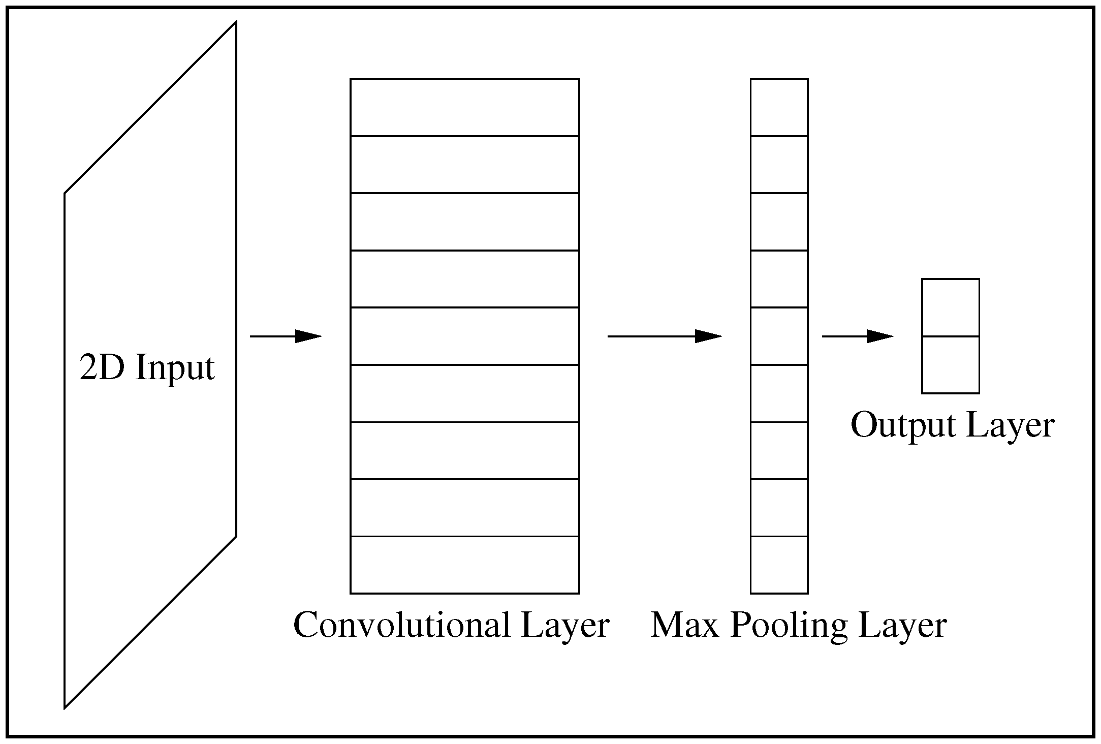
Article

A Simple Convolutional Neural Network with Rule Extraction

Department of Computer Science, University of Applied Sciences and Arts of Western Switzerland, Rue de la Prairie 4, 1202 Geneva, Switzerland
Current address: University of Applied Sciences and Arts of Western Switzerland, Rue de la Prairie 4, 1202 Geneva, Switzerland.
Appl. Sci. 2019, 9(12), 2411; https://doi.org/10.3390/app9122411
Submission received: 24 April 2019 / Revised: 5 June 2019 / Accepted: 6 June 2019 / Published: 13 June 2019
(This article belongs to the Special Issue Advances in Deep Learning)

Abstract

:
Classification responses provided by Multi Layer Perceptrons (MLPs) can be explained by means of propositional rules. So far, many rule extraction techniques have been proposed for shallow MLPs, but not for Convolutional Neural Networks (CNNs). To fill this gap, this work presents a new rule extraction method applied to a typical CNN architecture used in Sentiment Analysis (SA). We focus on the textual data on which the CNN is trained with “tweets” of movie reviews. Its architecture includes an input layer representing words by “word embeddings”, a convolutional layer, a max-pooling layer, followed by a fully connected layer. Rule extraction is performed on the fully connected layer, with the help of the Discretized Interpretable Multi Layer Perceptron (DIMLP). This transparent MLP architecture allows us to generate symbolic rules, by precisely locating axis-parallel hyperplanes. Experiments based on cross-validation emphasize that our approach is more accurate than that based on SVMs and decision trees that substitute DIMLPs. Overall, rules reach high fidelity and the discriminative n-grams represented in the antecedents explain the classifications adequately. With several test examples we illustrate the n-grams represented in the activated rules. They present the particularity to contribute to the final classification with a certain intensity.

1. Introduction

Artificial neural networks learn by examining numerous examples many times. After training, it is very difficult to explain their decisions, because their knowledge is embedded within the values of the parameters and neuron activations, which are at first glance incomprehensible. Deep neural networks are at the root of the significant progress accomplished over the past five years in areas such as artificial vision, natural language processing and speech recognition. In addition, a number of studies have been conducted to clarify the potential of deep models, such as Convolutional Neural Networks (CNNs) in Sentiment Analysis (SA) [1,2]. Nevertheless, the transparency of bio-inspired models is currently an open and important research topic, as in the long term, the acceptance of these models will depend on it. Furthermore, transparency is essential in relation to a recent European General Data Protection Regulation (GDPR), which also presents a right of explanation. Specifically, when an automated decision is taken by a system, one has the right to request a meaningful explanation.
Neural networks being considered as black-boxes have been made transparent by techniques that were first applied to shallow Multi Layer Perceptrons (MLPs). A natural way to explain MLP responses is through the use of propositional rules [3]. Andrews et al. introduced a taxonomy describing the general characteristics of all rule extraction methods [4]. Later, a desire to make neural network ensembles transparent became apparent and several techniques were proposed. Bologna introduced the Discretized Interpretable Multi Layer Perceptron (DIMLP) to generate symbolic rules from both single networks and ensembles [5,6]. The key idea behind rule extraction in DIMLPs is the precise localization of axis-parallel discriminative hyperplanes [5,6,7,8]. A brief explanation is provided in Section 3.2.
Recently, many works involving deep neural networks have gained momentum. On one hand, many techniques aiming at explaining CNN decisions in image classification are based on visualization of areas that are mainly relevant for the outcome [9], but as stated by Rudin [10]: “it does not explain anything except where the network is looking”. On the other hand, the purpose of several methods is to learn an interpretable model in the local region close to an input instance [11]. Adadi and Berrada presented a comprehensive overview of Explainable Artificial Intelligence (XAI), including neural networks [12]. In addition, a survey on black-box models with its “explanators” is proposed by Guidotti et al. [13]. The state of the art highlights a lack of global methods aiming at extracting symbolic rules from CNNs. Local methods could represent good candidate techniques, in order to define a global algorithm that may aggregate all local models in an ensemble. Currently, the approach of generating rules from aggregated local models has not been tackled, since ensembles tend to be more opaque than single models. Note however that it could be carried out by the same technique used in [6].
In this article we propose a rule extraction technique for a CNN, typically used in Sentiment Analysis [2] with textual data. Our technique is not restricted to local regions, but it is global to all the samples of the input space. The layers of this network are: A two-dimensional input layer representing sentences by means of word embeddings [14]; a convolutional layer; a max-pooling layer; and finally a fully connected layer. After the training phase, the fully connected layer is replaced by a DIMLP [7] that makes it possible to generate propositional rules. The DIMLP subnetwork approximates the fully connected part of the original CNN to any desired precision. The antecedents of the extracted rules represent maximal responses of convolutional filters. By propagating the rules back to the input layer, it is possible to determine the discriminative combination of words in the decision-making process. These words are structured into n-grams that depend on the size of the convolutional filters. As a result, each antecedent in a rule is given as: “if an n-gram in a sentence is present and maximal with respect to the list of possible n-grams, then...”. As an example, with the sentence “Hilarious, touching and wonderfully dyspeptic.”, the following rule with several n-grams is activated (Symbol “-” separates the words composing an n-gram; it is worth noting that punctuation is also taken into account.): “if hilarious and hilarious-, and hilarious-,-touching and touching-and-wonderfully and wonderfully-dyspeptic-. then POSITIVE.
This article extends our recent approach proposed in [15]. Specifically, the rule extraction algorithm is formalized and more details are provided. The experimental part is now based on cross-validation with many more examples of extracted rules. We also define a measure that makes it possible to determine for each rule antecedent its contribution to the final classification. Finally, a comparison with decision trees and SVMs has been carried out; it shows that our approach is more accurate. In the following paragraphs, Section 2 illustrates a number of representative works aiming at giving insight into deep architectures, Section 3 describes the proposed model with the CNN architecture and the DIMLP subnetwork, then we present the experimental results, followed by the conclusion.

2. Related Work

In the next paragraphs we give a non-exhaustive view of representative works aiming at explaining deep networks classifications. First, we briefly describe techniques applied to deep networks different from CNNs. Then, a number of representative methods related to CNNs are described.

2.1. Rule Extraction from Deep Networks without Convolution

Garcez and Tran proposed the first method of rule inference from Deep Beliefs Networks (DBN) [16]. In this stochastic network model, Boolean formulas were generated from two successive layers with a certain level of confidence. Overall, rules were generated by chaining down the boolean formulas from the output layer to the input layer. Recently, Hayashi trained DBNs and then transferred the last layer of weights into MLPs having a unique hidden layer [17]. Rules were generated from shallow MLPs by the Re-RX algorithm [18].
Zilke proposed a rule extraction technique applied to deep networks of stacked auto-associators [19,20]. Specifically, rules were first generated by decision trees between two successive layers. Subsequently, rules putting into play the input layer and the output layer were formed by transitivity. Similarly, in [21,22] the author generated rules from deep DIMLPs based on stacked auto-encoders.

2.2. Explanation of CNN Classifications

On object recognition problems, Hendriks et al. explained CNN classifications by training a second network that learns to produce sentences as an explanation feature [23]. Specifically, it learned to generate sentences that realized a global sentence property by reinforcement learning. Babiker et al. proposed to generate a heat map from a CNN to localize important regions of the image for classification [24]. The key idea behind this approach is the use of the Kullback-Leibler divergence gradient. Lapuschkin et al. introduced Layer-wise Relevance Propagation (LRP) to determine the inherent reasoning of deep neural networks [25]. In practice, this technique generated heatmaps of relevant areas contributing to the final classification. Furthermore, the authors characterized the importance of the context, with respect to targeted objects in images. For medical images, Holzinger et al. used very deep CNN architectures with residuals [3]. To understand the internal structure of the trained networks, they proposed to replace the majority of convolutional layers by AM-FM components (Amplitude Modulation-Frequency Modulation) and to retrain the upper network layers. Overall, convolution layers were visualized through their frequency coverage.
Zeiler and Fergus presented DeconvNet [26], in which strong activations are propagated backward to determine parts of the image causing these activations. Mahendran and Vedaldi proposed an optimization method based on image priors to invert a CNN [27]. As a result, visualizations yielded insight on the information represented at each layer. Dosovitskiy and Brox proposed to analyze which data is preserved by a feature representation and which data is discarded [28]. Specifically, from a feature vector a neural network was trained to predict the expected pre-image, corresponding to the average image producing the given feature vector.
Several authors proposed to interpret CNNs in the neighborhood of the instances. As an example, Ribeiro et al. presented LIME (Locally Interpretable Model Agnostic Explanations), whose purpose is to learn an interpretable model in the local region close to an input instance [11]. A first disadvantage of this approach is that the data must be transformed into binary format. Secondly, local explanations were only provided through linear models and their features relevance. Similarly Turner et al. introduced the Model Explanation System [29]. Basically, by using a Monte Carlo technique, they derived a scoring system for finding the best explanation. Koh et al. determined the training instances that are the most important for the prediction [30]. Finally, LORE (Local Rule Based Explanations) learns a local decision tree on a synthetic neighborhood generated through a genetic algorithm [13]; then, rules are generated to explain the outcome, as well as counterfactual rules.
Frosst and Hinton proposed to use a CNN to train a particular decision tree that imitates the input-output associations found out by the trained CNN [31]. Nevertheless, the decision tree did not explain the network logic, clearly. As an improvement, Zhang et al. proposed a decision tree to explain CNN predictions at the semantic level [32]. Specifically, the decision determines with respect to image recognition tasks, which filters are activated by objects parts and how much they contribute to the final classification. Overall, their technique provided an approximate explanation of CNN classifications.
The Explanation of CNNs responses in text classification has been rarely explored, as stated in [33]. The authors show that one-dimensional convolution filters can be associated to different semantic classes of n-grams. Moreover, the max-pooling layer is able to separate important n-grams. In [34] the Layer-wise Relevance Propagation (LRP) estimates which individual words are relevant to the overall classification decision.

2.3. Differences and Similarities with Our Approach

Many approaches aiming at explaining CNN classifications are based on the visualization of image areas that are mainly relevant to the result. A recent survey on this topic is presented in [9]. Guidotti et al. present a comprehensive survey of techniques aimed at elucidating deep neural networks [13]. In their view, explanators of black-box models include decision trees, symbolic rules but also other entities like: Features Importance (FI) and Sensitivity Analysis. Specifically, the latter allows the inspection of the black-box by observing changes in the classification result when varying inputs. FI is a measure representing the importance of the inputs, which is very often related to the coefficients resulting from trained linear models. Note that both Sensitivity Analysis and FI highlight specific properties of the model, without necessitating an overall understanding of it.
Our ultimate goal is to determine propositional rules, because they are close to the logic used by humans. Moreover, with the use of symbolic rules, discrimination between different classes is explained through rule antecedent values. This is much more precise than simply characterizing the relevant image subregions, because the way in which discrimination between different classes is carried out is undetermined [10]. The main difference between our method and the most recent techniques described in [12,13] aiming at generating decision trees or symbolic rules from deep neural networks is that our method is global and the others are local.
With respect to the taxonomy introduced by Andrews et al. [4] describing the general characteristics of all rule extraction methods, pedagogical techniques would be able to potentially generate symbolic rules from any neural network architecture (globally or locally). Specifically, a pedagogical method learns the associations between the input layer and the classification responses of the black-box model, without taking into account the values of its weights. Subsequently, rules can be generated, since the model that has been trained to recognize input-output associations is transparent. Examples of pedagogical techniques are reported in [35,36]. Despite their potential, pedagogical techniques have been applied to deep architectures like CNNs, very rarely [31]. It is worth noting that our rule extraction technique is not pedagogical, since it belongs to the ‘eclectic’ category [4].
Eclectic techniques are both pedagogical and decompositional. The latter category involves that the transparent model is generated by analyzing weight values of the neural network model. Note that the majority of decompositional techniques suffers from exponential algorithmic complexity [6]. As a result, in many cases a pruning step is carried out to reduce the number of weights. Hence, it seems very difficult to apply decompositional algorithms to CNN architectures. DIMLP rule extraction method has polynomial algorithmic complexity [8]. It is eclectic because weights of the first hidden layer define possible rule antecedents. In a second step these rule antecedents are confirmed or rejected in the rules by a pedagogical algorithm.

3. Proposed Model

3.1. CNN Architecture

A CNN architecture is composed of several successive layers of neurons. Specifically, in this work we use:
  • a two-dimensional input layer;
  • a convolutional layer;
  • a max-pooling layer;
  • a fully connected layer.
This network model shown in Figure 1 is very similar to that proposed in [2]. The only structural difference is the number of fully connected layers, which is equal to one in this work and equal to two in Figure 1. The different layers are described with more details in the following paragraphs.

3.1.1. Two-Dimensional Input Layer

A two-dimensional input layer is used to encode text. As shown by Figure 2, several words are represented on the vertical axis. Horizontally, a single word could be viewed as a boolean vector with zeros everywhere, except for a component whose value is equal to one. However, a drawback is the fact that thousands of components are typically required. A more parsimonious coding is achieved by word embeddings [14]. Specifically, a word is not anymore a boolean vector, but a vector with continuous values of typical size equal to 300. It is worth noting that the dimensionality of word embeddings is often between 100 and 300. As stated in [37], 300 is one of the most adopted sizes in various studies.

3.1.2. Two-Dimensional Convolutional Layer and Max-Pooling Layer

A key element in CNNs is based on the convolution operator. Given a two-dimensional kernel w p , q of size PxQ and a data matrix of elements x a , b , the calculation of an element c i j of the convolutional layer is
c i j = f ( p P q Q w p , q · x i + p , j + q + b p , q ) ;
with f a transfer function and b p , q the bias. As a transfer function we use a hyperbolic tangent:
tanh ( x ) = exp ( 2 x ) - 1 exp ( 2 x ) + 1 .
We define S p and S q as the stride parameters along the horizontal and vertical axis between two successive convolutions. In this work S p = S q = 1 . Moreover, we require the kernel to be completely inside the sample matrix (without zero padding). As an example, with data samples of size 6 × 6 and P = Q = 3 , the resulting convoluted map has size 4 × 4.
Figure 3 illustrates a particular case of convolution with respect to a text matrix of size 7 × 5 and a kernel of size 4 × 5. This kernel moves over the text matrix, carrying out an element-wise multiplication with the part of the data it is currently on. This is repeated by sliding down the kernel by one position, vertically. Hence, the result of convolution is a vector of four components. “Wide convolution” is the denotation when the horizontal size of the kernel is equal to the horizontal size of the data matrix. With wide convolution, the size of a kernel is defined as its vertical size. For instance, in Figure 3 the kernel size is equal to four.
A remarkable relationship is fulfilled between the size of the kernels and the number of consecutive words taken into account by the convolution operator. Since the size of a kernel is the number of components on the vertical axis, it corresponds to the number of consecutive words processed at any position in a sentence. As an example, three consecutive words are denoted as ’trigrams’ and can be detected by kernels of size three. Similarly, two consecutive words are called ’bigrams’ and can be taken into account by kernels of size two. Finally, to emphasize single words it is possible to define filters of size one.
The max-pooling layer reduces the size of a vector or a matrix by applying a “Max” operator over non-overlapping regions. Figure 4 illustrates in the left a number of vectors obtained after convolution. From each vector the maximal value is extracted and concatenated in a new layer, which enables n-gram position invariance.

3.1.3. Fully Connected Layer

In this work, a unique fully connected layer of weights follows the max-pooling layer. First, a dot product of s l scalars is calculated:
s l = k ( v k l · m k ) .
Symbol m k represents vector components of the max-pooling layer and v k l is a matrix term of weight coefficients, the bias being included in the sum. Then, a Softmax activation function is applied. Specifically, for a number N of s i scalars it calculates an N-dimensional vector with values between 0 and 1:
o l = exp ( s l ) k exp ( s k ) ;
with o l as the activation of a neuron in the output layer. The architecture of the CNN used in this work is summarized in Table 1. Specifically, I designates the input layer, C represents the convolutional layer with 40 kernels for each size (this value has been fixed empirically, without trying to reach the possible best predictive accuracy). ( C 1 , C 2 , C 3 ), M is the max-pooling layer (120 neurons), and O designates the output layer including two neurons. Each word is coded in a vector of 300 components, with a maximum number of words per sample equal to 59.
To train the network, the loss function is the cross-entropy (J); here we give its version for two classes:
J ( W ) = - p l t l ( p ) log ( o l ( p ) ) + ( 1 - t l ( p ) ) log ( 1 - o l ( p ) ) .
Symbol W represents all the network weights, index p is related to training samples, index l designates an index for the neurons of the output layer, o l ( p ) is the activation of an output neuron, and t l ( p ) represents a target value.

3.2. The DIMLP Model

DIMLP differs from a standard MLP in the number of connections between the input layer and the first hidden layer. Specifically, any hidden neuron receives only a connection from an input neuron and the bias neuron, while all other layers are fully connected [7]. The activation function above the first hidden layer of a typical DIMLP is a sigmoid function given as:
σ ( x ) = 1 1 + exp ( - x ) .
For the first hidden layer a step function or its generalization corresponding to a staircase activation function is used. For simplicity, we first give the step function τ ( x ) , which is a particular case of the staircase function with only one step:
τ ( x ) = 1 if   x > 0 ; 0 otherwise .
The key idea behind rule extraction from DIMLPs is the precise localization of axis-parallel discriminative hyperplanes. In other words, the input space is split into hyper-rectangles representing propositional rules. Specifically, the first hidden layer creates for each input variable a number of axis-parallel hyperplanes that are effective or not, depending on the weight values of the neurons above the first hidden layer. As an example, Figure 5 illustrates an elementary DIMLP network with a hidden neuron, a weight w between the input neuron and the hidden neuron and a bias b between the bias neuron and the hidden neuron. Because of the step function as the activation of the hidden neuron, a potential hyperplane discriminator lies in - b / w . It will depend on the layers above the first hidden layer, whether the hyperplane discriminator will be effective or not. Generally, these hyperplanes are parallel to the axis of the input neurons. Hence they represent possible rule antecedents.
The starting point of the rule extraction algorithm is the list of all potential hyperplane discriminators. The number of these hyperplanes depends on the number of stairs in the staircase activation function. Then, a decision tree is built and rules are generated from each tree path. Typically, at this stage the number of rules and antecedents is too large. Hence, a greedy algorithm progressively removes antecedents and rules. More details on the rule extraction algorithm can be found in [8].
Since the CNN defined in the previous Section is trained with a Softmax function in the output layer (cf. Equation (4)), we replace the sigmoid by it. As stated previously, the activation function in the first hidden layer of DIMLPs is a staircase function S ( x ) , with Θ stairs that approximate the Identity function ( I ( x ) ) on a compact interval:
I ( x ) = x ;
S ( x ) = R m i n , if   x R m i n ;
R m i n represents the abscissa of the first stair. By default R m i n = - 1 .
S ( x ) = R m a x , if   x R m a x ;
R m a x represents the abscissa of the last stair. By default R m a x = 1 . Between R m i n and R m a x , S ( x ) is:
S ( x ) = I ( R m i n + θ · x - R m i n R m a x - R m i n ( R m a x - R m i n θ ) ) .
Square brackets indicate the integer part function, with θ = 1 , Θ . The approximation of the Identity function by a staircase function depends on the number of stairs Θ . The larger the number of stairs the better the approximation.

3.3. The Interpretable CNN Architecture

The interpretable CNN architecture used in this work is illustrated in Table 2. Its layers are: I-C-M-H-O, with a DIMLP subnetwork included in layers M-H-O. Rule extraction is performed after the training of a CNN with layers I-C-M-O. Note that the CNN with layers I-C-M-H-O is not trained. Specifically, the weight matrix between layers M and O of the trained CNN is transferred to layers H and O of the CNN with layers I-C-M-H-O. Because of the Identity function between M and H, network I-C-M-H-O approximates network I-C-M-O to an arbitrary precision that depends on the number of stairs of the staircase activation function. Hence, rules can be generated from the DIMLP subnetwork. Yet, rule antecedents are related to layer M representing filter values. From that layer, discriminative combinations of words represented in the input layer have to be determined (see below).
Figure 6 depicts an example going from a tweet to a rule. First, each word of a sentence is provided to the input layer as horizontal vectors of numbers. Subsequently, these vectors are convolved by the convolutional layer; note that each rectangle on this layer represents a convolution filter. After convolution, the max-pooling layer takes over; its role is to simplify the processed data by retaining maximal values. From this layer to the output layer we have a DIMLP subnetwork. Hence, the extracted rule antecedents represent activation values of the the Max-Pooling layer. For clarity, those which are not represented in the rule at the bottom are left blank. Finally, the correspondence between antecedents and n-grams is shown at the bottom; the algorithm described below allows us to determine them.
Generally, many rule extraction techniques generate ordered rules, which means that rules are given in a sequential order, with two consecutive rules linked by an “else” statement. A long list of ordered rules involve many implicit antecedents that makes the interpretation difficult. Rules generated from the DIMLP subnetwork (M-H-O) are unordered. With this type of rules, the “else” statement is absent. Thus, each rule is considered as a single piece of knowledge that can be examined in isolation [38].
Each rule antecedent related to the max-pooling layer is given as a < t , or a t . Since a rule antecedent can be true with one or more n-grams in the input layer, it involves a disjunction of n-grams (one or more n-grams connected by a logical or). Nevertheless, for a given sample and with the use of the “Max” function in the M layer, a unique n-gram becomes dominant (the one with the highest activation). Before giving an algorithm that allows us to determine discriminative n-grams for a given sample, let us define several sets and variables:
  • G: Set of n-Grams generated from a dataset;
  • R: Set of rules (with respect to layer M);
  • R i : A rule in R;
  • A i j : An antecedent in R i ; specifically A i j = ( m j < c i j ) or A i j = ( m j c i j ) , with m j designating a neuron in the M layer and c i j ;
  • S k : A sample covered by R i ;
  • H: Set of n-Grams generated from S k ;
  • Γ : Set of sought discriminative n-grams ( Γ H ) ;
  • a c t ( . ) : The activation(s) of a specified neuron in layer M, with respect to one or more inputs in the input layer.
It is worth noting that with this CNN architecture the activation of neuron m j in the M layer depends solely on kernel K j in the C layer. Hence, given a sample S k covered by R i and its set of n-grams H, each discriminative n-gram related to antecedent A i j is found by characterizing the n-gram (in H) activating neuron m j the most. Given R i and S k , the following algorithm generates discriminative n-grams:
  • Γ =
  • For all A i j R i loop (w.r.t variable j)
  • G j = { g G H | A i j is true }
  • F j = { x q | q = G j , x = a c t ( G j ) for neuron m j }
  • f j = max( F j )
  • g j = { g G j | f j = a c t ( g ) for neuron m j }
  • Γ = Γ g j
  • end loop
For clarity let us explain the different steps of the algorithm specified above. First, its result will be stored in Γ , which is initialized as an empty set. Secondly, a main loop that iterates on all rule antecedents is defined. Subsequently, in step three, for each rule antecedent A i j we determine the n-grams of S k (a sample) that makes A i j true. Then, for each antecedent A i j the purpose is to determine the n-gram involving the highest activation of neuron m j in the M layer (steps four to six). For instance, with the antecedent f 113 0 . 24 of a particular rule generated from an interpretable CNN and a sentence given as “a real movie, about real people, that gives us a rare glimpse into a culture most of us don’t know”, four trigrams makes the antecedent true:
  • “culture most of” (0.251715)
  • “rare glimpse into” (0.257523)
  • “into a culture” (0.273310)
  • “us a rare” (0.311517)
the number after each trigram is the activation value of the 113th neuron in the M layer. The fourth trigram provides the highest activation, hence it is the detected trigram. Generally, it is plausible to obtain a global view of each extracted rule by characterizing for each antecedent its winning n-grams with respect to all the covered samples.
For a given rule antecedent and a given sample, it is useful to determine the linear contribution of each winning n-gram g j , with respect to the final classification. Specifically, this measure corresponds to the product of the filter activation in the M-layer multiplied by the weight connecting the neuron of highest activation in the output layer. The output neuron of strongest activation indicating the class, a positive value of this measure means that the n-gram contributes in favor of the classification, while a negative value is against it. The linear contribution is given as a function:
L C ( g j ) = v k · a c t ( g j ) ;
with act ( g j ) designating the activation of a neuron m k in the M layer and v k corresponding to a weight between m k and the output layer (the one related to the neuron of highest activation).

4. Experimental Results

In this section, we first present the general results on the accuracy of CNNs based on cross-validation. Secondly, Decision Trees (DTs) [39] are trained with CNN prediction classes instead of the true label. Thirdly, CNNs are compared to Support Vector Machines (SVMs) [40]. Subsequently, we replace DIMLP subnetworks by DTs. Then, representative examples of rules extracted from CNNs are shown. They emphasize how discriminative n-grams intuitively explain “tweet” classifications. Finally, we illustrate with two examples how to inspect rules, globally.

4.1. General Results

A CNN including a convolutional layer with 120 kernels of size one, two and three was defined empirically (cf. Section 3.1.3). Note that our purpose was not to find the best possible CNN architecture, but rather to create an acceptable CNN in terms of performance and then to generate rules to explain classifications. Training was performed with Lasagne libraries, version 0.2 [41]. The training parameters were:
  • learning rate: 0 . 02 ;
  • momentum: 0 . 9 ;
  • dropout = 0 . 2 ;
To illustrate the results of rule extraction, we applied the CNN architecture defined above to a well-known binary classification problem related to “tweets” of movie reviews [42]. The characteristics of the dataset are:
  • number of samples: 10,662;
  • maximal number of words in a “tweet”: 59;
  • positive sentiment samples: 5331;
  • negative sentiment samples: 5331;
  • single words: 21,426;
  • bigrams: 111,590;
  • trigrams: 174,628.
The positive and negative subsets have been divided into 10 folds, in order to carry out ten-fold cross validation trials. Moreover, a randomly selected subset of the training set representing 10% of it was extracted as a tuning set for early-stopping [43], which is useful to avoid over-training. Table 3 illustrates the results. The first row of this Table is related to the original CNN, while the other ones provide results obtained by interpretable CNNs, which depend on the number of stairs in the staircase activation function. Columns from left to right designate:
  • average train accuracy;
  • average predictive accuracy on the testing set;
  • average fidelity, which is the degree of matching between generated rules and the CNN;
  • average predictive accuracy of the rules;
  • average predictive accuracy of the rules when rules and CNN agree;
  • average number of extracted rules;
  • average number of rule antecedents.
The average predictive accuracy of the rules is slightly lower than that obtained by the CNN (73.7% versus 74.1%, for the best result). Moreover, average fidelity on the testing set is above 95%, meaning that rules explain CNN responses in a large majority of cases. Finally, the best average predictive accuracy of the rules when rules and model agree is higher than that obtained by the CNN (75.1% versus 74.1%).
As a baseline, a simple pedagogical technique aiming at explaining CNN predictions is represented by a DT that learns training samples with CNN prediction classes, instead of true labels. Table 4 illustrates the results obtained by cross-validation. The λ parameter, which is the minimum number of samples required to be at a leaf node makes it possible to control the size of the trees. The number of nodes of a tree is in turn related to the proportion of learned training samples. It is worth noting that the fidelity on the training samples decreases when λ is increased. Moreover, the average predictive accuracy is never above 60%, the average fidelity being always below 63%. On one hand, this performance is substantially lower than that obtained by interpretable CNNs with DIMLP subnetworks (see Table 3). On the other hand, with λ 10 , a lower number of rules are generated.
We may wonder about replacing the DIMLP subnetwork in interpretable CNNs by Decision Trees, from which rules can be extracted. Note that a decision tree can be viewed as a set of rules, with each rule represented by a path going from the root to a leaf. Table 5 illustrates the results with respect to the extracted rules, by varying the λ parameter. The best average predictive accuracy is equal to 68.6%, which is much lower that that obtained by CNNs with the DIMLP subnetwork (68.6% versus 73.7%). An intuitive reason explaining this result is that the fully connected layer of the original CNN is better approximated by DIMLPs than DTs. However, DTs generate a significant smaller number of rules, on average: 201.8 versus 573.8.
Support Vector Machines are usually very competitive with very highly dimensional classification problems. Here we have 17,700 ( 59 300 ) input variables for each sample; thus, a natural question is whether SVMs perform better than CNNs. Due to the high input dimensionality it is recommended to use linear SVMs. Table 6 present the results by varying the C parameter, which controls the proportion of misclassified training samples [44]. The best average predictive accuracy is less than that obtained by interpretable CNNs (70.6% versus 73.7%). A question arising is whether this difference is statistically significant.
A multiple statistical comparison test is performed to find out whether average predictive accuracies are significantly different. With an ANOVA statistical test we aim at determining whether all the models used here obtain the same average predictive accuracy against the alternative hypothesis that they are not all the same. In other words, the null hypothesis states that the means are all equal. For this statistical test we define a significance level equal to 0.01, which involves a 1% risk of concluding that a difference exists when there is no actual difference. Not surprisingly, ANOVA rejects the null hypothesis that all model average predictive accuracies are equal (p-value = 3 . 1252 · 10 - 59 ) .
At this point it is within reach to compare a subset of the models, such as the SVMs related to their highest average predictive accuracy and interpretable CNNs. These results are shown in Table 7. The small p-values involve that with very high probability the predictive accuracy of the rules generated from each interpretable CNN is significantly different from the one measured on SVMs with C parameter equal to 0.01. Similar results are illustrated in Table 8, with respect to SVMs with C parameter equal to 0.005.

4.2. Examples of Detected N-Grams from the Rules

First, rules are expressed with antecedents given as filter responses. Then, n-grams are determined from the antecedents. Specifically, the truthfulness of the antecedents involve long lists of n-grams. Nevertheless, for a given sample and a given rule antecedent, only a unique n-gram “wins the competition” (cf. Section 3.3). Rules are ranked according to their support with respect to the training set, which corresponds to the number of covered samples. Finally, rules are not disjointed, which means that a sample can activate more than a rule.

4.2.1. Discriminative N-Grams Determined from R 26

We first illustrate rule number 26 ( R 26 ), with support equal to 464 samples with respect to the training set and 47 samples with respect to the testing set:
  • ( m 35 < 0 . 24 ) ( m 54 0 . 16 ) ( m 77 < 0 . 22 ) ( m 98 0 . 18 ) ( m 112 0 . 12 ) ( m 120 < 0 . 1 ) Class = NEGATIVE
Here, m i ( i = 1 , 120 ) designates neuron activations in the max-pooling layer. Indexes between one and 40 are related to single words, those between 41 and 80 correspond to bigrams, and those between 81 and 120 involve trigrams. The accuracy of this rule is 93.3% on the training set and 87.2% on the testing set.
In the following Figures are depicted examples of “tweets” belonging to the testing set and including the discriminative n-grams, ranked according to the linear contribution in the output layer (cf. Equation (12)). Figure 7 shows a correctly classified “tweet” related to R 26 . Single words, bigrams and trigrams are illustrated vertically. A “*” or a “+” designates a repeated n-gram, since two different antecedents are able to code the same n-gram. In Figure 7 “too-bad-the” is a trigram, “too-bad” is a bigram and “style” is a single word. Note that “style” and “style-.” (punctuation is also coded in word embeddings) are against the final classification. The most contributing n-gram is “too-bad-the”, which appears twice. In this case, all n-grams containing “bad” contribute to the negative polarity. This fact is also in agreement with our common sense.
Figure 8 illustrates another example in which the most contributing n-gram to the final classification is a trigram: “mediocre-special-effects”. Note that this is also in accordance with our perception. Bigram “worst-of” is the second most contributing n-gram. Surprisingly, single word “worst” is almost neutral with respect to the final classification.
Figure 9 shows that the most discriminative n-gram is trigram “so-mind_numbingly-awful”, then follows bigram “so-mind_numbingly”. Note also that three n-grams are against the final classification. Among them, single word “as” is the strongest element in contradiction with the final classification.
As a last example for rule R 26 , we can see in Figure 10 that trigram “just-bad-;” and bigram “just-bad” are the most contributing n-grams. Again, “as” is the strongest element in favor of the positive polarity (thus, in contradiction with the “tweet” classification).

4.2.2. Discriminative N-Grams Determined from R 24

As a second rule, R 24 is:
  • ( m 29 < 0 . 18 ) ( m 54 < 0 . 26 ) ( m 93 < 0 . 16 ) ( m 95 < 0 . 18 ) ( m 110 0 . 22 ) ( m 113 0 . 24 ) ( m 118 < 0 . 20 ) Class = POSITIVE
Its accuracy is 93.4% on the training set with support equal to 469 samples and 98.0% on the testing set, with support equal to 51 samples. Figure 11 depicts a covered “tweet” in the testing set. The most important n-gram is trigram “has-a-subtle”, which is evoked by two different antecedents. Moreover, n-grams related to “it’s over” are associated to negative polarities.
In Figure 12, we illustrate a “tweet” that is more difficult to classify, since it starts in a rather negative manner and then becomes strongly positive. As a consequence, the CNN detects a considerable number of negative elements. Four n-grams are not in favor of the correct classification, with two of them including “not”. Overall, the contribution of the positive parties is stronger, with a strongest trigram related to two different antecedents (“offers-gorgeous-imagery”).
Figure 13 illustrates a short “tweet”. Two trigrams appear twice and surprisingly single word “entertaining” contributes negatively to the final class. In Figure 14 the strongest n-gram is: “beautifully-accomplished-lyrical”, which is very complimentary. Curiously, bigram “beautifully-accomplished” is slightly negative in its contribution to the final class. This would indicate a defect in the classifier, as well as “entertaining” in the previous “tweet”. An explanation for the negative connotation of this single word would be that it appears 31 times in the dataset of negative “tweets”. Finally, Figure 15 illustrates a testing case, which is wrongly classified by the CNN, but correctly classified by R 24 . Here, “is-a-feast” is the only element that contributes positively to the classification.

4.3. Global View of Rules

A rule antecedent can be true with several different n-grams. Hence, to analyze a rule as a whole we must detect its related n-grams for each antecedent and for all covered samples. Note that a rule with antecedents depending on neuron activations in the M-layer can be formulated in the input layer as:
  • “if one of the n-grams related to the first antecedent is present and maximal (Only the n-gram that activates the most its related neuron in the M layer is the one that makes the antecedent true.) then ⋯” and ⋯ “if one of the n-grams related to the last antecedent is present and maximal then ⋯”.
Let us give a first example with a rule covering a moderate number of tweets in the training set. We take into account a CNN network with parameter Θ equal to 100. Rule 347 ( R 347 ) presents two antecedents. It covers 32 samples in the training set and it is given by:
  • ( m 36 0 . 28 ) ( m 110 0 . 28 ) Class = POSITIVE;
with m 36 and m 110 representing neurons in the M-layer. Antecedent m 36 is related to five single words: “cinema”; “see”; “you”; “you’ll”; “your”. Antecedent m 110 is related to 31 different trigrams, with five of them starting with “is” (“is-a-beautiful”, “is-a-compelling”, “is-a-satisfying”, “is-a-startling”, “is-a-sweet”, “is-the-heart”); four trigrams starting with “it’s” (“it’s-a-beautiful”, “it’s-a-smart”, “it’s-a-sweet”, “it’s-a-very”); three trigrams starting with “yet” (“yet-deeply-watchable”, “yet-sensual-entertainment”, “yet-shadowy-vision”); two trigrams starting with “warm” (“warm-and-charming”, “warm-your-heart”), and 17 other trigrams (“touching-and-tender”, “simple-,-sweet”, “intriguing-and-beautiful”, etc.). Note that these n-grams clearly belong to the class of positive polarity.
Another example with a rule covering more samples is represented by rule R 66 (253 samples in the training set):
  • ( m 74 0 . 12 ) ( m 84 < 0 . 24 ) ( m 110 0 . 28 ) Class = POSITIVE;
Antecedent m 74 is related to 155 distinct bigrams. About two thirds of them start with “a” or “an” or “and” (for instance: “a-perfect”; “an-amusing”, “and-touching”). Other bigrams start with “deeply”, such as: “deeply-moving”; “deeply-absorbing”; “deeply-moving”; “deeply-touching”, etc. Finally, “surprisingly” is also present in five bigrams (“surprisingly-charming”, “surprisingly-engaging”, “surprisingly-manages”, “surprisingly-powerful”, “surprisingly-touching”).
Regarding m 110 , similarly to R 347 in which this antecedent is present, we see many trigrams starting with “is” or “it’s”. Other trigrams having several times the same first word starts with: “charming”; “deeply”; “funny”; “heart”; “intelligent”; “intriguing”; “lovely”; “offers”; “powerful”; “smart”; “surprisingly”; “touching”; “warm”; “yet”; etc. For antecedent m 84 we also have a certain number of trigrams starting with “is” or “it’s”, though significantly less than previously. Moreover, we counted more than 40 trigrams starting with “,” and more than 20 trigrams starting with “and”. Other non-numerous trigrams with the same first word start with: “a”; “but”; “film”; “in”; “melodrama”; “movie”; “smart”; “surprisingly”; “that”; “smart”.
Since we generate unordered rules, each rule can be viewed as a single classifier that can be analyzed without considering the other rules. The more the number of rule antecedents and samples covered, the longer the examination will take. However, in principle this is always possible. Specifically, by looking at the n-grams related to each antecedent it is realizable to understand in which context a rule is applied.

4.4. Discussion

DTs were not as good as DIMLPs at approximating the fully connected layer at the top of the original CNN. Nevertheless, more rules were generated from DIMLPs. Thus, the best approximation precision is at the cost of more complicated rulesets. With DIMLPs it would be feasible to alleviate the size of extracted rulesets with the use of reduced training sets, as it was carried out in [22].
The linear contribution of n-grams is a measure that allows us to characterize the relative importance of discriminative combinations of words. On one hand, it helps to characterize flaws in the classifier, such as the detection of n-grams that contribute to an opposite class. On the other hand, it enables to understand which word combinations are used correctly. The contribution of n-grams is easily calculated with only a unique fully connected layer, but an open question is to find a way to calculate it with a greater number of fully connected layers. A solution to this problem could be the use of a feature importance value, as described in the framework reported in [45].
To determine a rule as a whole, it is sufficient to characterize all discriminative n-grams over all covered samples. From the linear contributions it is plausible to determine the n-grams that go against the rule class. Then, flaws can be detected and possibly a corrective strategy could be developed with the use of additional training examples putting into play problematic n-grams.
The CNN architecture used in this work is simple, as it includes a unique convolutional layer. We might wonder whether our rule extraction technique could be adapted to more complex architectures used in object recognition, such as LeNet [46], AlexNet [47], and VGGNet [48]. In a similar manner to what has been achieved here, we would extract unordered rules at the level of the first fully connected layer. Given a sample and a rule activated by this sample, it would be conceivable for each rule antecedent to determine one or more image regions that contribute positively or negatively to the final classification. The extent of these regions would be characterized by going back to the input layer, after passing through an arbitrary number of convolutional and max-pooling layers.

5. Conclusions

We presented a new rule extraction technique applied to a CNN in sentiment analysis. Our approach is global and could be extended to object recognition problems encompassing a moderate number of convolutional layers. Our rule extraction method consisted in approximating a trained CNN by transforming the top layers into a transparent neural network model. Thus, rules generated from the transparent subnetwork were propagated backward to the input layer and became comprehensible, as the antecedents represent n-grams. The rules can be inspected globally, by determining for each antecedent all the related n-grams, or locally, by characterizing for a given sample the discriminative n-grams that contribute to the final classification. These n-grams allowed us to explain with several examples why the classifier worked well or badly. In the future it will be interesting to determine how to correct flaws in a neural network with the help of the extracted rules. One way could be to inject supplementary training examples, aiming at modifying the linear contributions of discriminative n-grams.

Funding

This research received no external funding.

Conflicts of Interest

The author declares no conflict of interest.

Abbreviations

The following abbreviations are used in this manuscript:
SASentiment Analysis
CNNConvolutional Neural Network
DIMLPDiscretized Interpretable Multi Layer Perceptron
MLPMulti Layer Perceptron
SVMSupport Vector Machines
DTDecision Trees
FIFeatures Importance

References

  1. Kim, Y. Convolutional neural networks for sentence classification. arXiv 2014, arXiv:1408.5882. [Google Scholar]
  2. Cliche, M. BB_twtr at SemEval-2017 Task 4: Twitter Sentiment Analysis with CNNs and LSTMs. arXiv 2017, arXiv:1704.06125. [Google Scholar] [Green Version]
  3. Holzinger, A.; Biemann, C.; Pattichis, C.S.; Kell, D.B. What do we need to build explainable AI systems for the medical domain? arXiv 2017, arXiv:1712.09923. [Google Scholar]
  4. Andrews, R.; Diederich, J.; Tickle, A.B. Survey and critique of techniques for extracting rules from trained artificial neural networks. Knowl.-Based Syst. 1995, 8, 373–389. [Google Scholar] [CrossRef]
  5. Bologna, G. A study on rule extraction from several combined neural networks. Int. J. Neural Syst. 2001, 11, 247–255. [Google Scholar] [CrossRef]
  6. Bologna, G. Is it worth generating rules from neural network ensembles? J. Appl. Log. 2004, 2, 325–348. [Google Scholar] [CrossRef] [Green Version]
  7. Bologna, G. Rule extraction from a multilayer perceptron with staircase activation functions. In Proceedings of the IEEE-INNS-ENNS International Joint Conference on Neural Networks (IJCNN 2000), Como, Italy, 27 July 2000; Volume 3, pp. 419–424. [Google Scholar]
  8. Bologna, G. A model for single and multiple knowledge based networks. Artif. Intell. Med. 2003, 28, 141–163. [Google Scholar] [CrossRef]
  9. Zhang, Q.S.; Zhu, S.C. Visual interpretability for deep learning: A survey. Front. Inf. Technol. Electron. Eng. 2018, 19, 27–39. [Google Scholar] [CrossRef]
  10. Rudin, C. Please Stop Explaining Black Box Models for High Stakes Decisions. arXiv 2018, arXiv:1811.10154. [Google Scholar]
  11. Ribeiro, M.T.; Singh, S.; Guestrin, C. Why should i trust you? Explaining the predictions of any classifier. In Proceedings of the 22nd ACM SIGKDD International Conference on Knowledge Discovery and Data Mining, San Francisco, CA, USA, 13–17 August 2016; pp. 1135–1144. [Google Scholar]
  12. Adadi, A.; Berrada, M. Peeking inside the black-box: A survey on Explainable Artificial Intelligence (XAI). IEEE Access 2018, 6, 52138–52160. [Google Scholar] [CrossRef]
  13. Guidotti, R.; Monreale, A.; Ruggieri, S.; Pedreschi, D.; Turini, F.; Giannotti, F. Local rule-based explanations of black box decision systems. arXiv 2018, arXiv:1805.10820. [Google Scholar]
  14. Mikolov, T.; Chen, K.; Corrado, G.; Dean, J. Efficient estimation of word representations in vector space. arXiv 2013, arXiv:1301.3781. [Google Scholar]
  15. Bologna, G. A Rule Extraction Study Based on a Convolutional Neural Network. In International Cross-Domain Conference for Machine Learning and Knowledge Extraction; Springer: Cham, Switzerland, 2018; pp. 304–313. [Google Scholar]
  16. Tran, S.N.; Garcez, A.D. Knowledge extraction from deep belief networks for images. In Proceedings of the IJCAI-2013 Workshop on Neural-Symbolic Learning and Reasoning, Beijing, China, 3–9 August 2013. [Google Scholar]
  17. Hayashi, Y. Use of a Deep Belief Network for Small High-Level Abstraction Data Sets Using Artificial Intelligence with Rule Extraction. Neural Comput. 2018, 30, 3309–3326. [Google Scholar] [CrossRef] [PubMed]
  18. Setiono, R.; Baesens, B.; Mues, C. Recursive neural network rule extraction for data with mixed attributes. IEEE Trans. Neural Netw. 2008, 19, 299–307. [Google Scholar] [CrossRef]
  19. Zilke, J. Extracting Rules from Deep Neural Networks. Master’s Thesis, Computer Science Department, Technische Universitat Darmstadt, Darmstadt, Germany, 2015. [Google Scholar]
  20. Zilke, J.R.; Mencía, E.L.; Janssen, F. DeepRED—Rule extraction from deep neural networks. In International Conference on Discovery Science; Springer: Cham, Switzerland, 2016; pp. 457–473. [Google Scholar]
  21. Bologna, G.; Hayashi, Y. A rule extraction study on a neural network trained by deep learning. In Proceedings of the IEEE 2016 International Joint Conference on Neural Networks (IJCNN), Vancouver, BC, Canada, 24–29 July 2016; pp. 668–675. [Google Scholar]
  22. Bologna, G.; Hayashi, Y. Characterization of symbolic rules embedded in deep DIMLP networks: A challenge to transparency of deep learning. J. Artif. Intell. Soft Comput. Res. 2017, 7, 265–286. [Google Scholar] [CrossRef]
  23. Hendricks, L.A.; Akata, Z.; Rohrbach, M.; Donahue, J.; Schiele, B.; Darrell, T. Generating visual explanations. In European Conference on Computer Vision; Springer: Cham, Switzerland, 2016; pp. 3–19. [Google Scholar]
  24. Babiker, H.K.B.; Goebel, R. Using KL-divergence to focus Deep Visual Explanation. arXiv 2017, arXiv:1711.06431. [Google Scholar]
  25. Lapuschkin, S.; Binder, A.; Montavon, G.; Muller, K.R.; Samek, W. Analyzing classifiers: Fisher vectors and deep neural networks. In Proceedings of the IEEE Conference on Computer Vision and Pattern Recognition, Las Vegas, NV, USA, 27–30 June 2016; pp. 2912–2920. [Google Scholar]
  26. Zeiler, M.D.; Fergus, R. Visualizing and understanding convolutional networks. In European Conference on Computer Vision; Springer: Cham, Switzerland, 2014; pp. 818–833. [Google Scholar]
  27. Mahendran, A.; Vedaldi, A. Understanding deep image representations by inverting them. In Proceedings of the IEEE Conference on Computer Vision and Pattern Recognition, Boston, MA, USA, 7–12 June 2015; pp. 5188–5196. [Google Scholar]
  28. Dosovitskiy, A.; Brox, T. Inverting visual representations with convolutional networks. In Proceedings of the IEEE Conference on Computer Vision and Pattern Recognition, Las Vegas, NV, USA, 27–30 June 2016; pp. 4829–4837. [Google Scholar]
  29. Turner, R. A model explanation system. In Proceedings of the 2016 IEEE 26th International Workshop on Machine Learning for Signal Processing (MLSP), Salerno, Italy, 13–16 September 2016; pp. 1–6. [Google Scholar]
  30. Koh, P.W.; Liang, P. Understanding black-box predictions via influence functions. arXiv 2017, arXiv:1703.04730. [Google Scholar]
  31. Frosst, N.; Hinton, G. Distilling a neural network into a soft decision tree. arXiv 2017, arXiv:1711.09784. [Google Scholar]
  32. Zhang, Q.; Yang, Y.; Wu, Y.N.; Zhu, S.C. Interpreting CNNs via decision trees. arXiv 2018, arXiv:1802.00121. [Google Scholar]
  33. Jacovi, A.; Shalom, O.S.; Goldberg, Y. Understanding Convolutional Neural Networks for Text Classification. arXiv 2018, arXiv:1809.08037. [Google Scholar] [Green Version]
  34. Arras, L.; Horn, F.; Montavon, G.; Müller, K.R.; Samek, W. “What is relevant in a text document?” An interpretable machine learning approach. PLoS ONE 2017, 12, e0181142. [Google Scholar] [CrossRef] [PubMed]
  35. Craven, M.; Shavlik, J.W. Extracting tree-structured representations of trained networks. In Advances in Neural Information Processing Systems; MIT Press: Denver, CO, USA, 1996; pp. 24–30. [Google Scholar]
  36. Augasta, M.G.; Kathirvalavakumar, T. Reverse engineering the neural networks for rule extraction in classification problems. Neural Process. Lett. 2012, 35, 131–150. [Google Scholar] [CrossRef]
  37. Yin, Z.; Shen, Y. On the dimensionality of word embedding. In Proceedings of the Advances in Neural Information Processing Systems, Montréal, QC, Canada, 3–8 December 2018; pp. 887–898. [Google Scholar]
  38. Lakkaraju, H.; Bach, S.H.; Leskovec, J. Interpretable decision sets: A joint framework for description and prediction. In Proceedings of the 22nd ACM SIGKDD International Conference on Knowledge Discovery and Data Mining, San Francisco, CA, USA, 13–17 August 2016; pp. 1675–1684. [Google Scholar]
  39. Quinlan, J.R. C4.5: Programs for machine learning. morgan kaufmann publishers, Inc., 1993. Mach. Learn. 1994, 16, 235–240. [Google Scholar]
  40. Vapnik, V.N.; Vapnik, V. Statistical Learning Theory; Wiley: New York, NY, USA, 1998; Volume 1. [Google Scholar]
  41. Dieleman, S.; Schlüter, J.; Raffel, C.; Olson, E.; Sønderby, S.K.; Nouri, D.; Maturana, D.; Thoma, M.; Battenberg, E.; Kelly, J.; et al. Lasagne: First Release; Zelando: Genève, Switzerland, 2015. [Google Scholar]
  42. Pang, B.; Lee, L. A sentimental education: Sentiment analysis using subjectivity summarization based on minimum cuts. In Proceedings of the 42nd Annual Meeting on Association for Computational Linguistics, Barcelona, Spain, 21–26 July 2004; Association for Computational Linguistics; p. 271. [Google Scholar]
  43. Yao, Y.; Rosasco, L.; Caponnetto, A. On early stopping in gradient descent learning. Constr. Approx. 2007, 26, 289–315. [Google Scholar] [CrossRef]
  44. Burges, C.J. A tutorial on support vector machines for pattern recognition. Data Min. Knowl. Discov. 1998, 2, 121–167. [Google Scholar] [CrossRef]
  45. Lundberg, S.M.; Lee, S.I. A unified approach to interpreting model predictions. In Proceedings of the Advances in Neural Information Processing Systems, Long Beach, CA, USA, 4–9 December 2017; pp. 4765–4774. [Google Scholar]
  46. LeCun, Y.; Bottou, L.; Bengio, Y. LeNet-5, Convolutional Neural Networks. 2015, p. 20. Available online: http://yann. lecun. com/exdb/lenet (accessed on 13 June 2019).
  47. Krizhevsky, A.; Sutskever, I.; Hinton, G.E. Imagenet classification with deep convolutional neural networks. In Proceedings of the Advances in Neural Information Processing Systems, Lake Tahoe, NV, USA, 3–6 December 2012; pp. 1097–1105. [Google Scholar]
  48. Simonyan, K.; Zisserman, A. Very deep convolutional networks for large-scale image recognition. arXiv 2014, arXiv:1409.1556. [Google Scholar]
Figure 1. The Convolutional Neural Networks (CNN) architecture used in this work. From left to right are shown a two-dimensional input layer, a convolutional layer, a max-pooling layer, and an output layer which is fully connected.
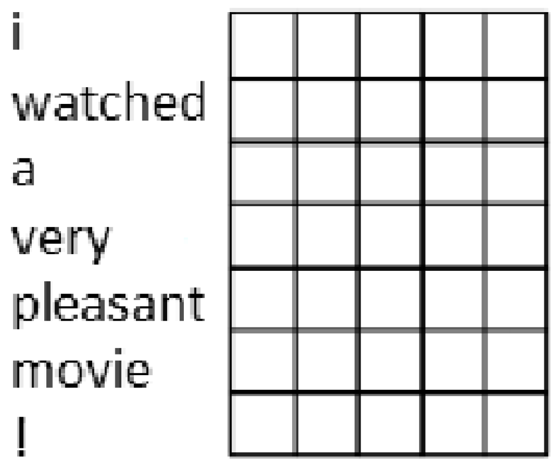
Applsci 09 02411 g001
Figure 2. Representation of text by a matrix of real numbers. A word is represented on the horizontal axis by word embeddings, while vertically several words are expressed.
Applsci 09 02411 g002
Figure 3. Wide convolution: The number of columns of the kernel is equal to the number of columns of the text matrix. The result of convolution (showed after the arrow) is a vector.
Applsci 09 02411 g003
Figure 4. The max-pool operator: The maximal value of each vector in the left is selected and concatenated in a new layer denoted as the “Max-pooling” layer (right most vector).
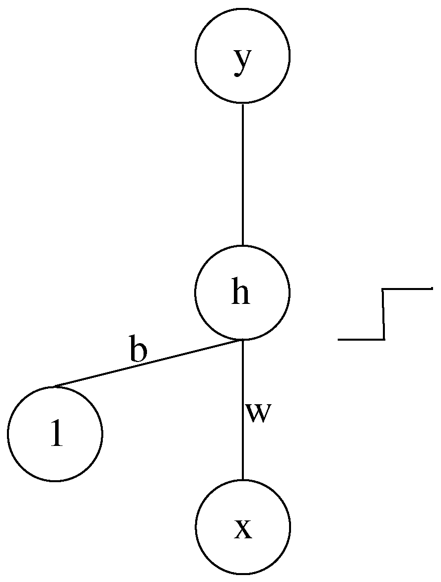
Applsci 09 02411 g004
Figure 5. A Discretized Interpretable Multi Layer Perceptron (DIMLP) network that potentially creates a discriminative hyperplane in - b / w . The activation function of the hidden neuron is a step function, while for the output neuron it is a sigmoid.
Applsci 09 02411 g005
Figure 6. Flow of data in the interpretable CNN (see the text for more details).
Applsci 09 02411 g006
Figure 7. N-grams determined from R 26 and the following “tweet” (in the testing set): “it is just too bad the film’s story does not live up to its style”. On the vertical axis are represented the n-grams classified according to their linear contribution. Negative values are against the final classification, while positive values are in its favor. The sum of the n-grams linear contributions is 0.435.
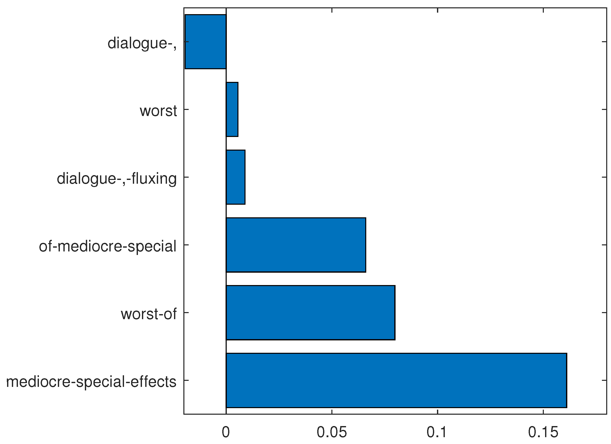
Applsci 09 02411 g007
Figure 8. N-grams determined from R 26 and the following “tweet”: “a zippy 96 min of mediocre special effects, hoary dialogue, fluxing accents, and—worst of all—silly-looking morlocks”. The sum of the n-grams linear contributions is 0.302.
Applsci 09 02411 g008
Figure 9. N-grams determined from R 26 and the following “tweet”: “so mind-numbingly awful that you hope britney won’t do it one more time, as far as movies are concerned”. The sum of the n-grams linear contributions is 0.211.
Applsci 09 02411 g009
Figure 10. N-grams determined from R 26 and the following “tweet”: “the tuxedo wasn’t just bad; it was, as my friend david cross would call it, hungry-man portions of bad.” The sum of the n-grams linear contributions is 0.283.
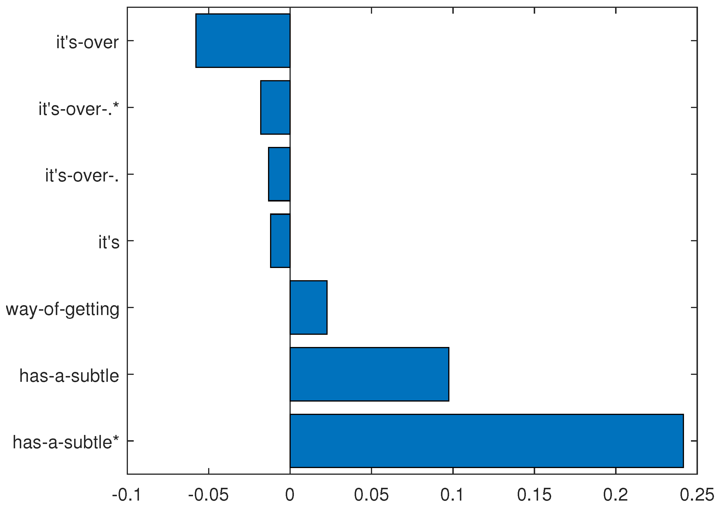
Applsci 09 02411 g010
Figure 11. N-grams determined from R 24 and the following “tweet”: “it has a subtle way of getting under your skin and sticking with you long after it’s over”. The sum of the n-grams linear contributions is 0.260.
Applsci 09 02411 g011
Figure 12. N-grams determined from R 24 and the following “tweet”: “though the controversial korean filmmaker’s latest effort is not for all tastes, it offers gorgeous imagery, effective performances, and an increasingly unsettling sense of foreboding.” The sum of the n-grams linear contributions is 0.251.
Applsci 09 02411 g012
Figure 13. N-grams determined from R 24 and the following “tweet”: “thoughtful, provocative and entertaining”. The sum of the n-grams linear contributions is 0.398.
Applsci 09 02411 g013
Figure 14. N-grams determined from R 24 and the following “tweet”: “it’s a beautifully accomplished lyrical meditation on a bunch of despondent and vulnerable characters living in the renown chelsea hotel . . .”. The sum of the n-grams linear contributions is 0.355.
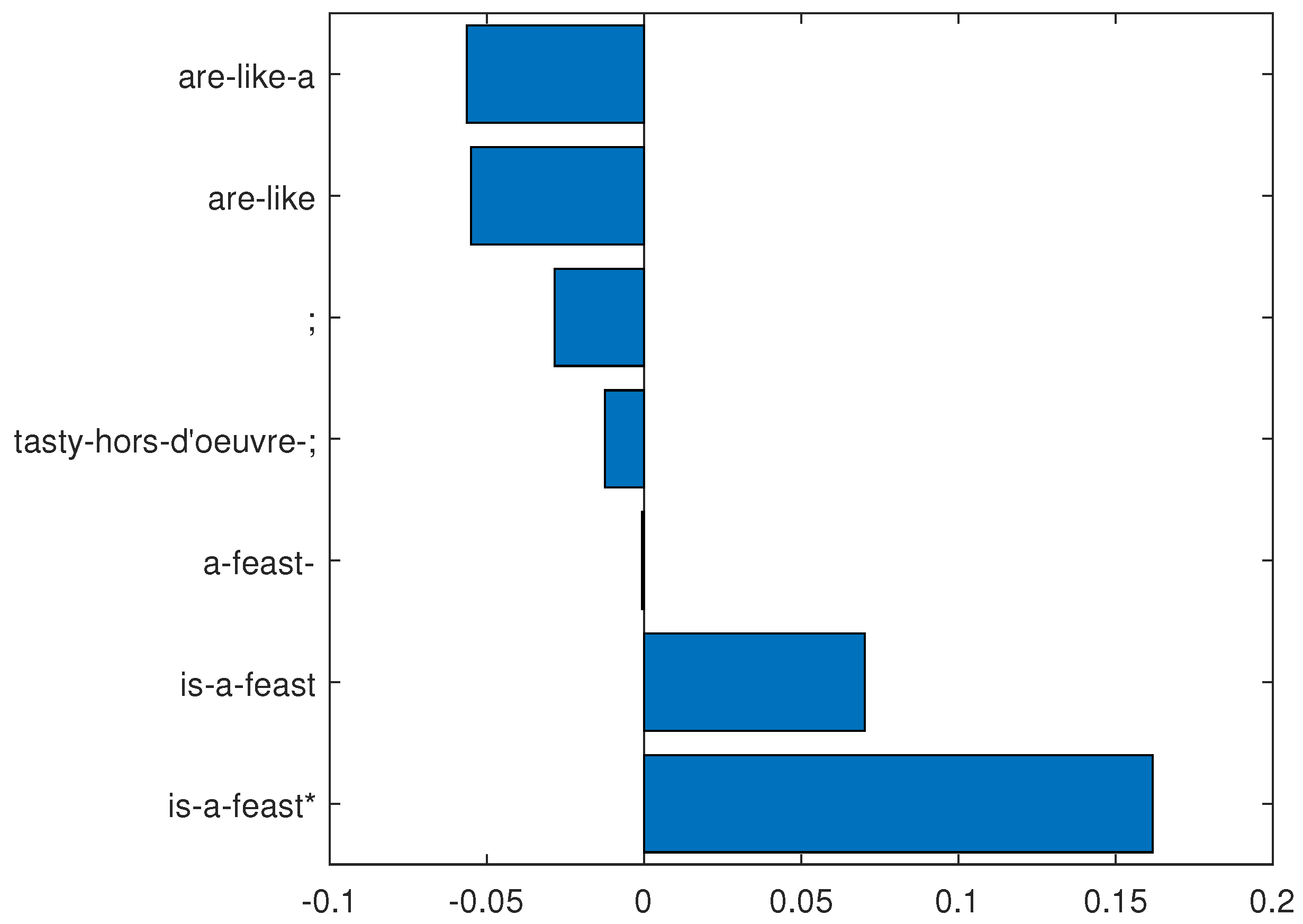
Applsci 09 02411 g014
Figure 15. N-grams determined from R 24 and the following “tweet” (in the testing set): “some movies are like a tasty hors-d’oeuvre; this one is a feast”. It is correctly classified by the rule, but wrongly classified by the network.
Applsci 09 02411 g015
Table 1. CNN architecture. Symbols for each layer are specified in the second row and sizes in the last.
InputConvolutionMax-Pooling LayerOutput
I C = ( C 1 , C 2 , C 3 ) MO
59 × 3001 × 300 × 40 2 × 300 × 40 3 × 300 × 401202
Table 2. Interpretable CNN architecture with symbols and sizes.
InputConv.Max-Pooling LayerDIMLP Hid. LayerOutput
IC = (C1, C2, C3)MHO
59 × 3001 × 300 × 40 2 × 300 × 40 3 × 300 × 401201202
Table 3. Average results based on cross-validation. The models are CNNs and interpretable CNN approximations with varying numbers of stairs in the staircase activation function. Standard deviations are given between parentheses.
 Tr. Acc.Tst. Acc.Fid.Rul. Acc. (1)Rul. Acc. (2)#Rul.#Ant.
CNN82.1 (1.3)74.1 (1.1)
CNN ( Θ = 100 )82.1 (1.3)74.1 (1.1)95.3 (0.6)73.7 (1.0)75.1 (1.0)651.7 (53.1)5368.9 (379.3)
CNN ( Θ = 200 )82.2 (1.4)74.1 (1.0)95.8 (0.4)73.7 (1.0)74.9 (1.0)573.8 (49.0)5040.7 (354.0)
CNN ( Θ = 500 )82.1 (1.4)74.1 (1.1)95.6 (0.8)73.6 (1.0)75.0 (0.9)566.1 (28.0)4980.7 (364.5)
Table 4. Average results obtained by Decision Trees (DTs) trained to learn datasets with CNN targets, instead of true labels. Columns from left to right represent average results on: Training accuracy; predictive accuracy; fidelity on the training set; fidelity on the testing set; number of extracted rules; and number of antecedents in the rules. In the rows, the  λ parameter controlling the size of the trees varies.
 Tr. Acc.Tst. Acc.Tr. Fid.Tst Fid.#Rul.#Ant.
DT ( λ = 1 ) 82.1 (1.3)57.5 (1.4)100.0 (0.0)60.9 (0.8)797.9 (16.9)10,354.3 (704.6)
DT ( λ = 5 ) 78.6 (1.1)57.9 (0.9)94.3 (0.2)61.0 (1.0)615.7 (6.4)7134.4 (304.6)
DT ( λ = 10 ) 75.6 (0.8)58.4 (1.3)89.1 (0.2)61.4 (1.3)456.8 (7.4)4863.7 (149.3)
DT ( λ = 15 ) 73.3 (0.7)58.5 (1.4)85.4 (0.4)61.6 (0.8)362.2 (5.6)3666.2 (116.4)
DT ( λ = 20 ) 71.9 (0.6)58.5 (1.5)82.9 (0.3)61.5 (2.2)299.5 (4.5)2904.5 (86.4)
DT ( λ = 25 ) 70.6 (0.6)58.6 (1.6)81.1 (0.4)61.4 (1.8)253.9 (3.5)2363.1 (71.6)
DT ( λ = 30 ) 69.8 (0.6)59.3 (1.0)79.8 (0.4)62.1 (1.8)222.7 (4.4)2015.9 (52.1)
DT ( λ = 35 ) 69.0 (1.0))59.3 (1.6)78.5 (0.4)62.5 (1.5)194.4 (4.2)1707.9 (64.1)
DT ( λ = 40 ) 68.5 (0.7)59.7 (1.8)77.4 (0.3)62.3 (1.4)173.9 (3.8)1482.8 (42.4)
DT ( λ = 50 ) 67.6 (0.6)59.6 (1.1)75.9 (0.4)62.7 (1.2)143.8 (2.7)1168.4 (31.5)
Table 5. Average results obtained by the rules generated from Decision Trees that replace the fully connected layer of CNNs. Columns from left to right represent average results on: Training accuracy; testing accuracy; number of extracted rules; number of antecedents in the rules. In the rows, the  λ parameter controlling the size of the trees varies.
 Tr. Acc.Tst. Acc.#Rul.#Ant.
DT ( λ = 1 ) 100.0 (0.0)66.0 (1.6)943.2 (23.6)11,160.8 (367.7)
DT ( λ = 5 ) 93.4 (0.2)66.8 (1.4)640.0 (16.3)6710.8 (191.2)
DT ( λ = 10 ) 89.0 (0.3)67.0 (1.4)450.4 (9.3)4414.5 (97.7)
DT ( λ = 15 ) 86.5 (0.4)67.6 (1.1)342.6 (5.6)3198.0 (60.5)
DT ( λ = 20 ) 84.8 (0.4)68.0 (1.0)276.8 (7.4)2483.2 (69.9)
DT ( λ = 25 ) 83.6 (0.4)67.9 (1.3)234.6 (4.7)2043.1 (38.4)
DT ( λ = 30 ) 82.7 (0.4)68.6 (0.9)201.8 (4.2)1704.5 (38.1)
DT ( λ = 35 ) 82.0 (0.5)68.3 (1.1)178.0 (3.5)1468.0 (40.1)
DT ( λ = 40 ) 81.3 (0.5)68.3 (1.2)159.1 (3.5)1281.6 (29.0)
Table 6. Average results obtained by Support Vector Machines (SVMs). Each row illustrates the accuracy results with respect to the C parameter.
 Tr. Acc.Tst. Acc.
SVM ( C = 0 . 005 ) 75.1 (0.1)70.5 (1.4)
SVM ( C = 0 . 01 ) 77.1 (0.2)70.6 (1.3)
SVM ( C = 0 . 05 ) 81.6 (0.2)70.2 (0.8)
SVM ( C = 0 . 1 ) 83.6 (0.3)69.9 (1.0)
SVM ( C = 0 . 5 ) 88.6 (0.2)68.1 (0.9)
SVM ( C = 1 ) 90.7 (0.2)67.5 (0.9)
Table 7. ANOVA comparison between CNNs and SVMs providing the better average predictive accuracy (equal to 70.6%).
 CNN Rul. Acc. (Average)CNN Rul. Acc. (Median)p-Value
CNN ( Θ = 100 ) and SVM ( C = 0 . 01 )73.773.8 1 . 0946 · 10 - 6
CNN ( Θ = 200 ) and SVM ( C = 0 . 01 )73.773.6 9 . 6623 · 10 - 7
CNN ( Θ = 500 ) and SVM ( C = 0 . 01 )73.673.9 1 . 5288 · 10 - 6
Table 8. ANOVA comparison between CNNs and SVMs providing the second better average predictive accuracy (equal to 70.5%).
 p-Value
CNN ( Θ = 100 ) and SVM ( C = 0 . 005 ) 8 . 8375 · 10 - 7
CNN ( Θ = 200 ) and SVM ( C = 0 . 005 ) 8 . 4786 · 10 - 7
CNN ( Θ = 500 ) and SVM ( C = 0 . 005 ) 1 . 0091 · 10 - 6

