Discriminating Emotions in the Valence Dimension from Speech Using Timbre Features

Featured Application

Emotion recognition from human speech is currently being used in a variety of different domains: in call centers, for analysis of customer’s satisfaction from services, in healthcare, monitoring stress or pain degree of patients in order to detect in an early stage of diseases and for better treatment. Moreover, it makes interaction more natural between humans and machines to analyze the behavior of drivers in cars with the teaching process.

Abstract

The most used and well-known acoustic features of a speech signal, the Mel frequency cepstral coefficients (MFCC), cannot characterize emotions in speech sufficiently when a classification is performed to classify both discrete emotions (i.e., anger, happiness, sadness, and neutral) and emotions in valence dimension (positive and negative). The main reason for this is that some of the discrete emotions, such as anger and happiness, share similar acoustic features in the arousal dimension (high and low) but are different in the valence dimension. Timbre is a sound quality that can discriminate between two sounds even with the same pitch and loudness. In this paper, we analyzed timbre acoustic features to improve the classification performance of discrete emotions as well as emotions in the valence dimension. Sequential forward selection (SFS) was used to find the most relevant acoustic features among timbre acoustic features. The experiments were carried out on the Berlin Emotional Speech Database and the Interactive Emotional Dyadic Motion Capture Database. Support vector machine (SVM) and long short-term memory recurrent neural network (LSTM-RNN) were used to classify emotions. The significant classification performance improvements were achieved using a combination of baseline and the most relevant timbre acoustic features, which were found by applying SFS on a classification of emotions for the Berlin Emotional Speech Database. From extensive experiments, it was found that timbre acoustic features could characterize emotions sufficiently in a speech in the valence dimension.

1. Introduction

A speech signal carries information not only connected with the lexical content, but also with the emotional state, age, and gender information of the speaker. Hence, speech signals can be used to recognize the emotional state of the speaker during communication with a machine.

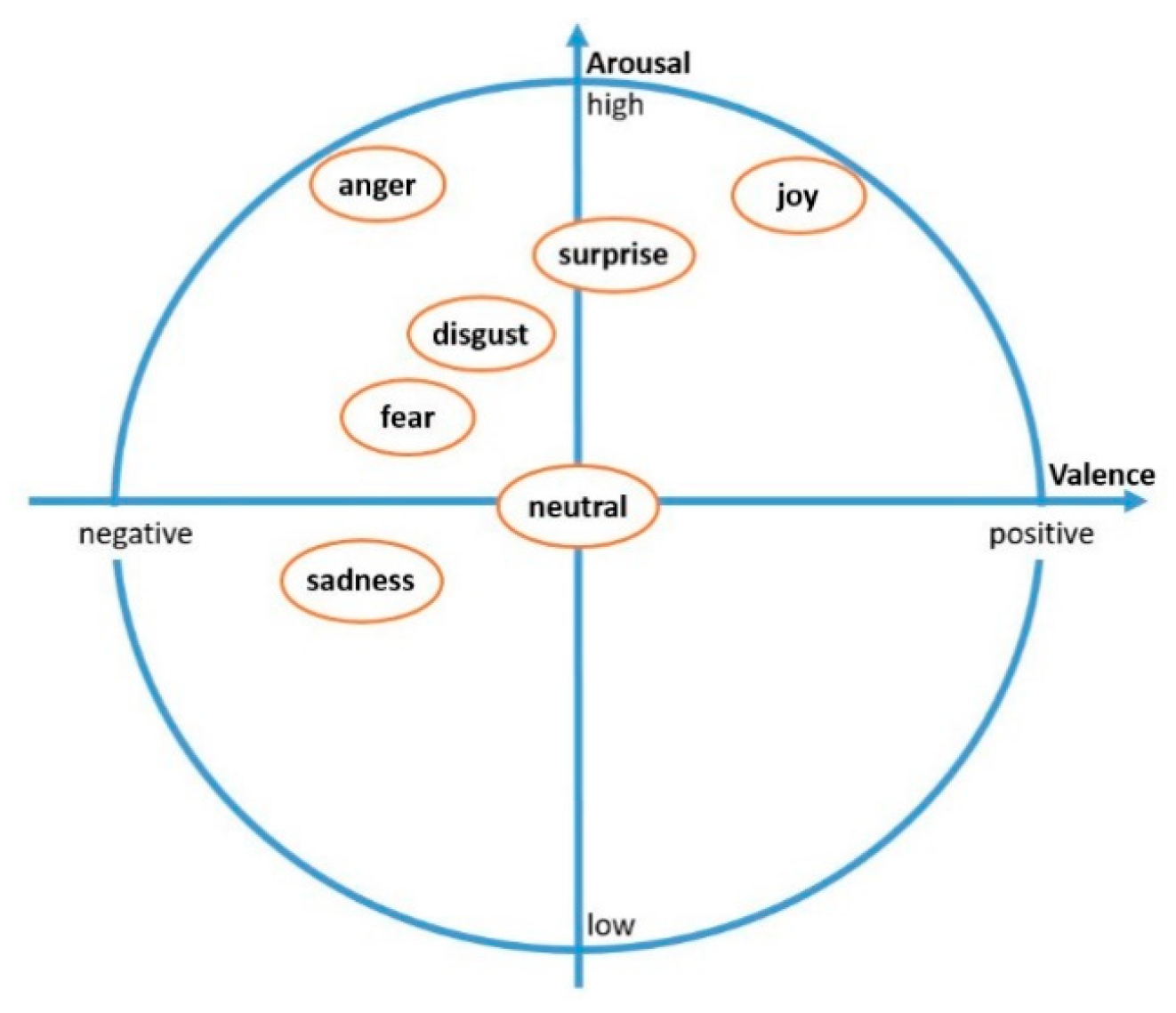
The automatic speech emotion recognition (SER) system needs an appropriate model to represent emotions. Human emotions can be modelled via the categorical approach, dimensional approach, and appraisal-based approach. In the categorical approach, emotions are divided into emotion categories: anger, happiness, fear, sadness, and so on. In the dimensional approach, emotions are represented by three major dimensions: valence (how positive or negative), arousal (how excited or apathetic) and dominance (dominant or submissive) [1,2]. Figure 1 illustrates seven basic emotions in arousal-valence dimensions [2].

The emotional states of the users can be recognized by a machine that uses sensory data, which comes from devices such as smartwatches, in order to detect the stress level of the users [3,4], or by extracting useful acoustic features of a speech wave. The acoustic features of emotional speech signal are well established in the arousal dimension and good results have been achieved in distinguishing high- and low-arousal emotions. For instance, Eyben et al. studied acoustic features in detail and proposed the geneva minimalistic acoustic parameter set (GeMAPS) [5]. In this study, more than ninety percent accuracy was achieved in binary arousal classification, but the accuracy was less than eighty percent with the binary valence classification. Several other studies [6,7,8] reported that discriminating emotions in the valence dimension was the most challenging problem. This problem is not only with the valence dimension but also with the discrimination of discrete emotions.

Communication between acoustic features of emotional speech and music was investigated in [9].

Table 1. Acoustic feature characteristics of discrete emotions expressed in speech and music performances.

Vocal Expression
Acoustic Features	Anger	Fear	Happiness	Sadness	Tenderness
speech rate	fast	fast	fast	slow	slow
voice intensity	high	high	high	low	low
voice intensity variability	high	high	high	low	low
high-frequency energy	high	high	high	low	low
F0	high	high	high	low	low
F0 variability	high	low	high	low	low
F0 contours	up	up	up	down	down
voice onsets	fast	fast	fast	slow	slow
microstructural regularity	irregular	irregular	regular	irregular	regular
Music Performance
tempo	fast	fast	fast	slow	slow
sound level	high	low	medium	low	low
sound level variability	high	high	low	low	low
high-frequency energy	high	low	medium	low	low
F0	sharp	sharp	sharp	flat	low
F0 variability	high	low	high	low	low
pitch contours	up	up	up	down	down
tone attack	fast	slow	fast	slow	slow
microstructural regularity	irregular	irregular	regular	irregular	regular

shows acoustic cues for discrete emotions expressed in speech and music performances. From Table 1, it is clear that most of the acoustic features of anger and happiness expressed in speech and music performances are similar. The prosodic, spectral, and excitation source features of emotional speech signals were analyzed for anger, happiness, neutrality, and sadness, and it was reported that those emotions share similar acoustic patterns [10,11,12]. Hence, there is more confusion in discriminating between those emotions. Busso et al. reported that spectral and fundamental frequency (F0) features discriminate emotions in the valence dimension more accurately [13].

Moreover, Goudbeek et al. reported that the mean value of the second formant was higher in positive emotions [14]. As the studies show, acoustic features related to the spectral and frequency of the speech signals can characterize emotions in the valence dimension better than acoustic features related to the intensity and energy of the speech signals.

Nevertheless, these acoustic features are not perfect. Thus, problems remain in discriminating emotions in the valence dimension. There are more than a hundred acoustic features. Hence, they need to be analyzed in order to find the best features that can characterize emotions in the valence dimension.

Timbre is known as a complex set of auditory attributes that describes the quality of a sound. Usually, timbre incorporates spectral and harmonic features of a sound [15]. It allows us to distinguish sounds even though they have the same pitch and loudness. For instance, when a guitar and a flute play the same note with the same amplitude, each instrument produces a sound that has a unique tone color [16]. Recently, timbre features have been analyzed for music emotion classification [17,18].

Furthermore, the effectiveness of timbre features has been explored for audio classification [19] and music mood classification [20], but it has not been analyzed for speech emotion recognition. In this paper, we analyzed timbre features to improve the recognition rate of emotions in a speech in the valence dimension. Furthermore, sequential forward selection (SFS) was applied to find the best feature subset among the timbre acoustic features. The effectiveness of the timbre features for speech emotion recognition was evaluated by compared to well-known MFCC and energy features of the speech signal.

Through the experiments, significant improvement was achieved using the selected best feature subset. Timbre features proved to be effective with the classification of discrete emotions and in the classification of emotions in the valence dimension. Average classification accuracy improvements of 24.06% and 18.77% were achieved with the binary valence classification and the classification of discrete emotions using the combination of baseline and timbre acoustic features on the Berlin Emotional Speech Database.

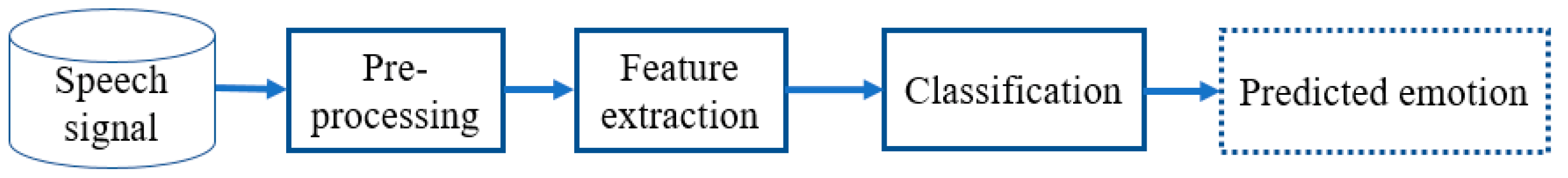
The rest of this paper is structured as follows: Section 2 gives information about related works that investigated acoustic features of a speech signal for emotion recognition. Section 3 describes general speech emotion recognition systems, acoustic feature extraction methods, and classification models. Emotion databases, the experiments, and the results are given in Section 4. Analysis of the results and discussion is presented in Section 5. Finally, Section 6 presents the conclusion of this work and future research directions.

2. Related Works

One of the most critical factors to consider when building an SER system is finding the most effective speech features to discriminate emotions from a speech signal. To solve this challenge, many researchers have investigated a massive number of speech features and achieved considerably good results in the arousal dimension (excited versus calm). For instance, CEICES systematically analyzed the acoustic features of speech to find the best acoustic feature set. They combined the acoustic features which they had and chose the best feature set based on classification accuracy.

In recent studies, the investigation of the acoustic features not only in the arousal dimension (excited versus calm), but also in the valence dimension (positive versus negative) has increased. Goudbeek and Scherer analyzed duration, F0, voice quality, and intensity features of an emotional speech signal to determine the role of those acoustic features regarding the arousal, valence, and potency/control emotional dimensions [21]. Their study showed that the variation of intensity of positive emotions was less than the variation of intensity of negative emotions. Moreover, positive emotions have a steeper spectral slope compared to negative emotions. Finally, they concluded that spectral shape features, and the speaking rate, which is related to rhythm, are the critical acoustic features for discriminating emotions in the valence dimension.

Eyben et al. [22] reported the importance of cepstral features (Mel frequency cepstral coefficients—MFCC). MFCC is closely related to spectral shape features. Speech features, such as energy, F0, voice quality, spectral, MFCC, and RASTA style-filtered auditory spectrum features of speech were analyzed to determine the relative effectiveness of these acoustic features in the valence dimension in [8]. They concluded that MFCC and RASTA style-filtered auditory spectra were the most relevant acoustic features for the valence dimension. Furthermore, the vital role of spectral shape and slope was studied and confirmed by [23,24].

Recently, Eyben et al. proposed the GeMAPS for voice research [5]. They chose acoustic features based on physiological changes in voice production, automatic extractability, and theoretical significance. This acoustic feature set included frequency-related (pitch, jitter), energy/amplitude related (shimmer, loudness), spectral (alpha ratio, spectral slope), and temporal (mean length, a rate of loudness peaks) features. They performed binary classification in the arousal and the valence dimensions using their minimalistic acoustic feature set and achieved 95.3% accuracy in the arousal dimension. Nevertheless, the highest accuracy was 78.1% in the valence dimension. This standard minimalistic acoustic feature set is much more powerful than other large-scale brute-force acoustic feature sets. Moreover, the most effective acoustic feature set in the field of SER so far was reviewed in [25].

Yildirim et al. reported that the most acoustic features were shared between anger and happiness, and between neutral and sad emotions [26]. Even though these pairs of emotions have a similar correlation in the arousal dimension, they are different in the valence dimension. Moreover, Juslin and Laukka investigated many acoustic features of speech and music to find the communication of emotions in vocal expressions and music performances, and they reported that most of the acoustic features of anger, happiness, and fear were the same (Table 1) [9], but we can differentiate between them in the valence dimension. Therefore, it is crucial to find the acoustic features that can differentiate emotions with similar energy, pitch, loudness, duration, and so on.

In recent years, along with exploring the speech features for SER, deep learning has been applied to various speech-related tasks. A trend in the deep learning community has emerged towards deriving a representation of the input signal directly from raw, unprocessed data. The motivation behind this idea is that the deep learning models learn an intermediate representation of the raw input signal automatically. For instance, in [27], a raw input signal and a log-mel spectrogram were used as an input to a merged deep convolutional neural network (CNN) to recognize emotion in speech. Furthermore, deep neural networks [28] and end-to-end multi-task learning for emotion recognition from raw speech signal [29] are recent examples of this approach. However, these frameworks might suffer from overfitting or from the limited size of the training data. In this work, we aimed to analyze the acoustic features of audio signals, which has not been explored for SER tasks.

The timbre model is used to distinguish two sounds with the same pitch and loudness in research into musical sounds. In general, timbre distinguishes between two sounds that have the same pitch and loudness [16]. Peeters proposed audio descriptors along with the acoustic feature extraction tool named Timbre Toolbox, which could potentially characterize the timbre of musical signals [30]. These audio descriptors comprise the temporal energy envelope (attack, decay, release), the spectral (spectral centroid, spread, slope), and the harmonic (harmonic energy, inharmonicity). Based on the theoretical, as well as the practical significance of these acoustic features of an emotionally expressed speech signal, we aimed to analyze them in the valence dimension as well as to classify discrete emotions in this paper.

3. Methodology

3.1. General Speech Emotion Recognition System

To automatically recognize emotions from a speech signal, there must be an SER system. The traditional SER system consists of three major parts, including pre-processing, feature extraction and classification, as shown in Figure 2.

In the pre-processing part, a signal processing technique, such as filtering, is performed to reduce the noise in a speech signal. It helps to enhance the overall accuracy of the SER system. Moreover, the speech signal is segregated into voiced and unvoiced regions in this part. The reason for this is to decrease the computational cost of feature extraction, as well as to obtain the meaningful part of a speech signal [31].

The objective of the feature extraction stage is to obtain a feature vector that can characterize the speech signal. This part is crucial in building the SER system. There is still no prevailing agreement regarding the features that are the most essential in discriminating emotions.

The final part of the SER system is classification. Generally, there are two primary classification approaches. The first includes static classification models, support vector machines (SVM) [32], and neural networks (NN) [33]. The second is the dynamic classification model, which is the hidden Markov model (HMM) [34]. Currently, static classification approaches predominate. The classification model is first trained with extracted features of an emotional speech signal on training data to optimize the model parameters, and then it is tested with the testing data to predict the emotion.

3.2. Acoustic Features

Acoustic features of a speech signal can be extracted from the whole utterance or a small part of a speech signal, which is called a frame. The acoustic features obtained from the entire utterance are called statistical acoustic features. Statistical acoustic features include the arithmetic mean, the standard deviation, the maximum, and the minimum. The advantage of these acoustic features is their amount. Because it is faster to apply a feature selection algorithm, their classification time is shorter. On the other hand, they may not be sufficient to optimize the parameters of complex classifiers, such as NN. Another group of acoustic features is local acoustic features, which are extracted from frames. These acoustic features can also be subdivided into frequency (pitch, jitter, formants), spectral (spectral slope, spectral flux, spectral energy), harmonic (harmonic energy, inharmonicity), and cepstral (MFCC) features, based on the domain extracted. For instance, MFCC is extracted after converting the time-amplitude signal into a time-frequency-magnitude signal and then into cepstrum. It is extracted from the cepstrum of a speech signal. Therefore, it is classified as a cepstral feature.

Many researchers have proved that MFCC is useful for distinguishing emotions on both the arousal and the valence dimension. It is estimated from the frequency domain using the mel scale, which is related to the human ear scale. The human ear scale is approximately linear up to around 1000 Hz, and logarithmic for frequencies above 1000 Hz [35].

To compute the MFCC feature vector, a speech signal is overtaken first through a filter to intensify the energy of a speech signal at a higher frequency. Then it is divided into frames (usually 30 ms short-time speech segments), and each frame is windowed with a hamming window to retain the continuity of the speech signal (1), where w[n] is the filter coefficient of the hamming window, L is the total amount of samples, and n is the current sample. After that, to convert the time domain speech signal into the frequency domain, as well as to obtain the magnitude frequency, Fast Fourier Transform (FFT) is performed. The next step is applying the mel-scale filter bank (2), where f is the frequency in Hertz, which is derived from a windowed frame of a speech signal.

$$w\left[n\right]=\{\begin{array}{ll}0.54-0.46\cos \left(\frac{2\mathsf{\pi }n}{L}\right)& \hfill 0\le n\le L-1\\ 0& \hfill \mathrm{otherwise}\end{array}$$

(1)

$$\mathrm{mel}\left(f\right)=1127\ln \left(1+f/700\right)$$

(2)

Then the log value of each of the mel spectrum is taken. Finally, a discrete cosine transform (DCT) is carried out to acquire the MFCC feature vector. The complete process of extracting the MFCC feature vector is shown in Figure 3.

Spectral features are derived from the spectral domain by converting a time-amplitude signal into a complex time-frequency-magnitude form using a short-term Fourier transform (STFT). STFT is calculated by performing a sliding window analysis over the speech signal. Next, the extraction method of the spectral features, which are analyzed in this work, is given. We indicate a speech signal with s(n) or s(t), where n is the sample number, t = n/sr is the time expressed in seconds, and sr is the sampling rate. We also indicate the frequency and magnitude of the spectrum of the speech signal as f(k) and a(t), respectively, where k is the frequency value between one and sr. The normalized form of $a\left(t\right)$ is calculated with Equation (3).

$$p\left(t\right)=\frac{a\left(t\right)}{{{\displaystyle \sum }}_{k=1}^{K}a\left(t\right)}$$

(3)

Spectral centroid is one of the statistical moments of the spectrum. It represents the spectral center of gravity and is computed with Equation (4). $p_k\left(t\right)$ is the normalized value of the magnitude STFT at frequency $k$ and time $t$.

$$u_{cent}\left(t\right)={\displaystyle \sum }_{k=1}^{K}f\left(k\right) p_k\left(t\right)$$

(4)

Spectral spread is another statistical moment of the spectrum. It is the spread of the spectrum around its mean value. It is calculated with Equation (5).

$$u_{spread}\left(t\right)={({\displaystyle \sum }_{k=1}^K{\left(f\left(k\right)-u_{cent}\left(t\right)\right)}^2 p_k\left(t\right))}^{1/2}$$

(5)

Spectral slope is how the energy of the spectral amplitude of a signal changes in different frequencies. Linear regression is applied to the spectral amplitude of a signal to get the spectral slope value, as in Equation (6). $a_k\left(t\right)$ is the amplitude value of the magnitude STFT at frequency $k$ and time $t$.

$$u_{slop}\left(t\right)=\frac{K{{\displaystyle \sum }}_{k=1}^{K}f\left(k\right) a_k\left(t\right)-{{\displaystyle \sum }}_{k=1}^{K}f\left(k\right)·{{\displaystyle \sum }}_{k=1}^K{a}_k\left(t\right)}{K{{\displaystyle \sum }}_{k=1}^{K}f{\left(k\right)}^2-{({{\displaystyle \sum }}_{k=1}^{K}f\left(k\right))}^2}$$

(6)

Spectral flatness is a measure of how noisy the signal is. We can measure it by dividing the geometrical mean by the arithmetical mean of the spectrum. If spectral flatness value is close to 1, the signal is considered noisy. It is computed with Equation (7).

$$u_{flat}\left(t\right)=\frac{{({{\displaystyle \prod }}_{k=1}^K{a}_k\left(t\right))}^{1/K}}{\frac{1}{K}{{\displaystyle \sum }}_{k=1}^K{a}_k\left(t\right)}$$

(7)

We grouped the acoustic features derived from sinusoidal harmonic partials of the speech signal as harmonic. They are calculated using a sinusoidal harmonic model. We indicate this with $a_h\left(t\right)$ and $f_h\left(t\right)$, which are the amplitude and frequency of partial $h$ at time $t$. H is the total number of partials.

Harmonic energy is the energy of the harmonic partials. It is calculated like computing the normal signal energy. However, this time, it is calculated from harmonic partials at a time $t$ (8).

$$E_H\left(t\right)={\displaystyle \sum }_{h=1}^H{(a_h\left(t\right))}^2$$

(8)

Noise energy is the difference between the total energy and harmonic energy (9).

$$E_N\left(t\right)=E_T\left(t\right)-E_H\left(t\right)$$

(9)

Noiseness is the measure of the degree to which the signal is harmonic or non-harmonic. When the value of noiseness is high, a signal is mainly non-harmonic. It is calculated using Equation (10).

$$nsr\left(t\right)=\frac{E_N\left(t\right)}{E_T\left(t\right)}$$

(10)

Tristimulus is a timbral equivalent to color attributes in vision. It consists of three different types of energy ratios. It helps to describe the first harmonics of the spectrum. It is calculated via Equation (11).

$$T_1\left(t\right)=\frac{a_1\left(t\right)}{{{\displaystyle \sum }}_{h=1}^H{a}_h\left(t\right)}, T_2\left(t\right)=\frac{a_2\left(t\right) + a_3\left(t\right) + a_4\left(t\right)}{{{\displaystyle \sum }}_{h=1}^H{a}_h\left(t\right)}, T_3\left(t\right)=\frac{{{\displaystyle \sum }}_{h=5}^H{a}_h\left(t\right)}{{{\displaystyle \sum }}_{h=1}^H{a}_h\left(t\right)}$$

(11)

Inharmonicity measures the departure of the frequencies of the partials $f_h$ from purely harmonic frequencies $h{f}_0$. It is calculated as the weighted sum of deviation of each partial from harmonicity. It is computed with Equation (12).

$$inharm\left(t\right)=\frac{2}{f_0\left(t\right)}\frac{{{\displaystyle \sum }}_{h=1}^H\left(f_h\left(t\right)-h{f}_0\left(t\right)\right){(a_h\left(t\right))}^2}{{{\displaystyle \sum }}_{h=1}^H{(a_h\left(t\right))}^2}$$

(12)

3.3. Classification Models

In the SER system, another crucial factor is the classification model. Many researchers have explored different types of classifiers, such as HMM, the Gaussian mixture model (GMM), k-nearest neighbors (KNN), the artificial neural network (ANN), and the SVM for the speech emotion recognition challenge [36]. Still, there is no common agreement on choosing the most powerful classifier for speech emotion classification. Each classification model has its own advantages and limitations. For this reason, the classification model must be selected depending on the problem.

In pattern recognition, as well as in classification problems, SVM is known to be one of the most efficient, simple, and widely used machine learning algorithms, especially for binary (two-class classification problems) classification (positive and negative, in our case) [37]. Moreover, it can also be extended to use in multiple classes problems. The basic idea is that it creates a hyperplane (or line) between the classes where the margin reaches the maximum value. The margin is the distance of the nearest training samples from the hyperplane. It can be trained through many training methods. One of them is empirical risk minimization. In this method, a discriminant function $g\left(x\right)$ is estimated from a finite set of examples by minimizing an error function (Equation (13)), where $R_{emp}$ is the training error, $z_k$ is the correct class, $g(x_k)$ is the predicted class, $w_1$ and $w_2$ are two different classes, and $n$ is the number of points in the dataset. This method is for linearly separable data. For the nonlinear problem, the kernel trick is applied to maximum-margin hyperplanes.

$$R_{emp}=\frac{1}{n}{\displaystyle \sum }_{k=1}^n{\left(z_k-g\left(x_k\right)\right)}^2; z_k=\{\begin{array}{cc}+1,\hfill & x_k\in w_1\hfill \\ -1,\hfill & x_k\in w_2\hfill \end{array}$$

(13)

In many recent studies, recurrent neural networks (RNNs) have been used for the SER task [38,39,40,41,42]. Ruben and Gloria [43] investigated the discriminative capabilities of RNNs in SER using low-level acoustic features of speech signals. RNNs are known to be useful in sequential data. Generally, deep neural networks (DNNs) use different parameters at each layer, but RNNs share the same parameters through all steps. However, they inadequately cover long context information because of the gradient vanishing problem. To solve this problem, a long short-term memory (LSTM) RNN was proposed [44], which consisted of recurrently connected memory blocks. In a recent study [45], different neural network architectures were evaluated for the SER task. They used spectrograms to train and evaluate deep learning models. The convolutional neural network (CNN) was used as a feature extractor and an LSTM-RNN was used as a classifier. In addition, in [46], emotions were recognized in both verbal and nonverbal speech sounds using DNN. In [38], statistical and local features were used to recognize emotions from speech. They also evaluated SVM and LSTM-RNN models and reported that the LSTM-RNN model outperformed the SVM with both the local and statistical features of an emotional speech. We also used SVM and LSTM-RNN classification models in our work.

4. Experiments

The analysis of acoustic features was performed both on the Berlin Emotional Speech Database (EMO-DB) and the Interactive Emotional Dyadic Motion Capture (IEMOCAP) database. Detailed information about emotional databases, acoustic feature extraction, and selection, as well as experiments, is given in the following sections.

4.1. Emotional Speech Databases

EMO-DB is one of the most frequently used emotional speech databases in SER, and it is a free public database [47] consisting of seven emotions, namely anger, happiness, neutrality, sadness, fear, boredom and disgust. The utterances in this database were created by ten (five male and five female) professional actors by speaking ten sentences in seven emotional states. We chose four emotions, namely anger, happiness, neutral, and sadness, for our experiments. The main reason for this was that these four emotions share similar acoustic features, and it is hard to discriminate these emotions in the valence dimension [26,48,49]. Moreover, these emotions are easily accessible in almost all other emotional speech databases. The number of utterances in each emotion category is different, meaning that the data are unbalanced. The number of utterances in the anger emotion is almost double that of the rest of the chosen emotions (anger (127), happiness (69), neutrality (78), and sadness (60)). To reduce data imbalance between numbers of instance in each emotion class, we randomly chose 78 utterances for anger emotion, and the number of utterances for the rest of the chosen emotions remained the same as mentioned above.

The IEMOCAP database is also popular and widely used to evaluate the proposed new methods as well as to analyze acoustic features in the SER [50]. It comprises both audio and visual data. This database is divided into five different sessions, and each session includes acted dialogues performed by two people. Each utterance has three categorical labels that are labeled by three annotators. We chose four emotions, namely anger, happiness, neutrality and sadness, and the utterances in each emotion category were chosen via the majority win method. This means that the utterance was selected when it was labeled with the same emotion by at least two annotators out of 3. We randomly chose 705 utterances for each selected emotion category to avoid an imbalanced data problem. Information about the databases, emotion categories and the number of files in each emotion category are given in

Table 2. Detailed information about the databases, emotion categories, and the number of samples in each emotion category.

Emotions	EMO-DB	IEMOCAP
	Number of Samples	Number of Samples
Anger	78	705
Happiness	69	705
Neutral	78	705
Sadness	60	705

.

4.2. Acoustic Feature Extraction and Selection

First, we extracted the most popular and most used acoustic features in the SER field, which include the MFCC, Energy, and their first-order derivatives, using open-source media interpretation by large feature-space extraction (openSMILE) [51]. Several studies have used MFCC acoustic features for speech emotion recognition [52,53,54]. We also considered those acoustic features as a baseline to evaluate our acoustic features. To extract energy and its first-order derivative, a speech signal was divided into short 30-ms frames with 10 ms overlapping. Then, the energy and its first-order derivative were extracted from each frame. The MFCC and its first-order derivative were extracted as shown in Figure 3.

We divided the acoustic features into three groups. The first group included MFCC, the energy and their first-order derivatives. We named this group the baseline acoustic features. The second group consisted of timbre features. The timbre features were extracted using the timbre toolbox [30] with MATLAB. In the timbre toolbox, both global (i.e., derived from the whole utterance) and local (i.e., extracted from frames) acoustic features can be extracted. Moreover, acoustic features can be extracted from different input representations (e.g., audio signal, short-term Fourier transform (STFT) amplitude and power, temporal energy envelope, and harmonic). We extracted local acoustic features from different input representations and experimented with them to find the most suitable input representation for our problem. The STFT (amplitude) and harmonic input representations were found to be the most suitable in our case through experiments. Classification accuracy was the criterion for choosing the most suitable input representations. Detailed information regarding extracting timbre features can be found in [30]. Our extracted timbre features consisted of 11 spectral features, which were derived from the STFT (amplitude), and 8 harmonic (the number of harmonics was set to 12) acoustic features. After extracting the timbre features, we also performed SFS [55] to find the best feature subset among all timbre acoustic features for the third group. In the SFS algorithm, the measure metric must be specified. It can be a particular error rate or classification accuracy. We chose classification accuracy as a measured metric. The working principle of this algorithm was as follows. In the first step, each acoustic feature is individually measured and the best one is chosen based on classification accuracy. A chosen feature remains in the second step, and then other features are added one by one. The best feature combination is selected in this step. After that, those chosen features are retained, and the others are added again one by one in the next step. The process goes on like this until the best feature subset is found. After performing the SFS, we found five spectral and four harmonic features for timbre. Finally, we had three groups of acoustic features. We named them baseline, timbre all, and timbre selected. The names of the acoustic features and their dimensions are given in

Table 3. Detailed information about acoustic features and their dimension.

Groups	Acoustic Feature Name	Dimension
Baseline	MFCC	16
	Delta MFCC	16
	Energy	1
	Delta Energy	1
Timbre all	Spectral Centroid	1
	Spectral Spread	1
	Spectral Skewness	1
	Spectral Kurtosis	1
	Spectral Slope	1
	Spectral Decrease	1
	Spectral Roll-off	1
	Spectral Flux	1
	Spectral Energy	1
	Spectral Flatness	1
	Spectral Crest	1
	Harmonic Energy	1
	Noise Energy	1
	Noiseness	1
	F0	1
	Inharmonicity	1
	Tristimulus	3
	Harmonic spectral deviation	1
	Odd to even harmonic ratio	1
Timbre selected	Spectral Centroid	1
	Spectral Spread	1
	Spectral Flux	1
	Spectral Energy	1
	Spectral Crest	1
	Noiseness	1
	F0	1
	Inharmonicity	1
	Tristimulus	3

.

4.3. Experimental Setup

To evaluate the four groups (baseline, timbre all, timbre selected, and combination of baseline and timbre selected) of acoustic features, we performed classification using the SVM and the LSTM-RNN classifiers. We divided the 4 categorical emotions into positive (happiness and neutral) and negative (anger and sadness) emotions, the same as in [5], to perform the binary valence classification. We also carried out classification for categorical emotions. SVM classification was carried out in MATLAB using machine learning and a deep learning toolbox. The kernel function was set to a radial base function (RBF) (Gaussian), gamma was set to automatic, and the c parameter was set to 1. Before feeding the data into the classifier, the z-score normalization was applied to each acoustic feature. To obtain more stable results, we performed a five-fold cross-validation (2 speakers in each fold) in our experiments. The LSTM-RNN classifier was built in a python programming language using the Keras [56] library. It consisted of 2 hidden layers with 256 nodes in each layer. For the activation function, relu was chosen with a 0.6 regularization parameter. The optimization function was Adam, and the loss function was a categorical cross entropy.

Firstly, classification was carried out for the baseline acoustic features. The average classification rates in all experiments are given in

Table 4. Average accuracy rate for all experiments for EMO-DB. (The bold numbers indicate the highest accuracy rate).

Acoustic Feature Set	Classifiers	Binary Valence	Discrete Emotions
Baseline	SVM	69.16%	74.72%
	LSTM-RNN	73.81%	77.72%
Timbre all	SVM	84.75%	85.67%
	LSTM-RNN	81.76%	86.58%
Timbre selected	SVM	85.58%	86.07%
	LSTM-RNN	80.33%	84.24%
Baseline + timbre selected	SVM	97.87%	96.2%
	LSTM-RNN	97.46%	96.49%

for the EMO-DB and in

Table 5. Average accuracy rate in all experiments for IEMOCAP. (The bold indicates the highest accuracy rate).

Acoustic Feature Set	Classifiers	Binary Valence	Discrete Emotions
Baseline	SVM	71%	57.3%
	LSTM-RNN	72%	58.58%
Timbre all	SVM	71%	60.39%
	LSTM-RNN	74%	65.06%
Timbre selected	SVM	68%	57.85%
	LSTM-RNN	72%	62.07%
Baseline + timbre selected	SVM	72%	59.75%
	LSTM-RNN	73%	63.03%

for the IEMOCAP. All results were obtained by testing each file and applying the majority win method. For instance, if the speech signal with the anger emotion consisted of 190 frames and the classifier predicted 100 frames as an anger emotion, we considered this file to be an anger emotion. We performed five-fold cross-validation (each fold consists of 2 speakers) to get more stable results. Each time 4 folds were used for training and the remaining one was used for testing. The accuracy was taken from each fold, and the final accuracy was calculated by adding the accuracies for each fold and dividing by 5.

The second experiment was performed using the timbre all acoustic feature set in order to determine the efficiency of the feature set. After that, an SFS algorithm was applied to the timbre all acoustic feature set to find the best feature subset. The third experiment was carried out with the timbre selected acoustic feature set. Finally, the last experiment was performed using a combination of the timbre selected and baseline acoustic feature sets in order to validate whether these acoustic feature sets complemented each other or overlapped.

5. Results and Discussion

One of the primary challenges in pattern recognition is finding the best features that can be correctly discriminated with recognition. In speech recognition, as well as in emotion recognition from speech, MFCC and energy are known to be the most useful acoustic features. Moreover, GeMAPS can be considered a standard acoustic feature set in music classification, speech recognition, and the SER [5]. However, some emotions are difficult to discriminate using MFCC and energy, such as anger and happiness. In most previous studies [48,49,57], classification accuracy of the happy emotion was low. The best accuracy rate (86.7%) was achieved using a large-scale brute-force acoustic feature set (6373 acoustic features), and 78.1% accuracy was achieved using extended GeMAPS for binary valence classification on EMO-DB [5]. Although the highest accuracy rate was achieved using a large-scale brute-force acoustic feature set, it is too difficult in terms of extraction time to use those features for real-time speech emotion recognition systems. The numbers of extracted features, along with the extraction time, are also crucial factors to consider when training pattern models and building a real-time speech emotion recognition system.

First, we examined the results for the EMO-DB. In our experiment, 97.87%, which was the highest accuracy rate (Table 4), was obtained using the combination of baseline and timbre selected acoustic features for binary valence classification. The combination of the baseline and timbre selected acoustic features sets also gave the highest accuracy rate for discrete emotions classification. The difference in accuracy rate between the timbre all and timbre selected acoustic feature sets was less than 2%. However, the number of acoustic features in timbre selected was almost two times less than the number of features in the timbre all feature set. This means that irrelevant features in timbre were all removed when the SFS was applied. The results were improved for the combination of the baseline and timbre selected acoustic feature sets compared to the rest of the acoustic feature sets. Consequently, it was clear that baseline and timbre features complemented each other.

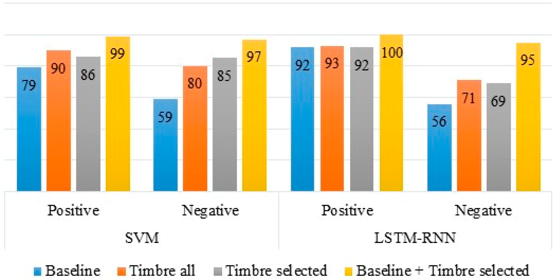
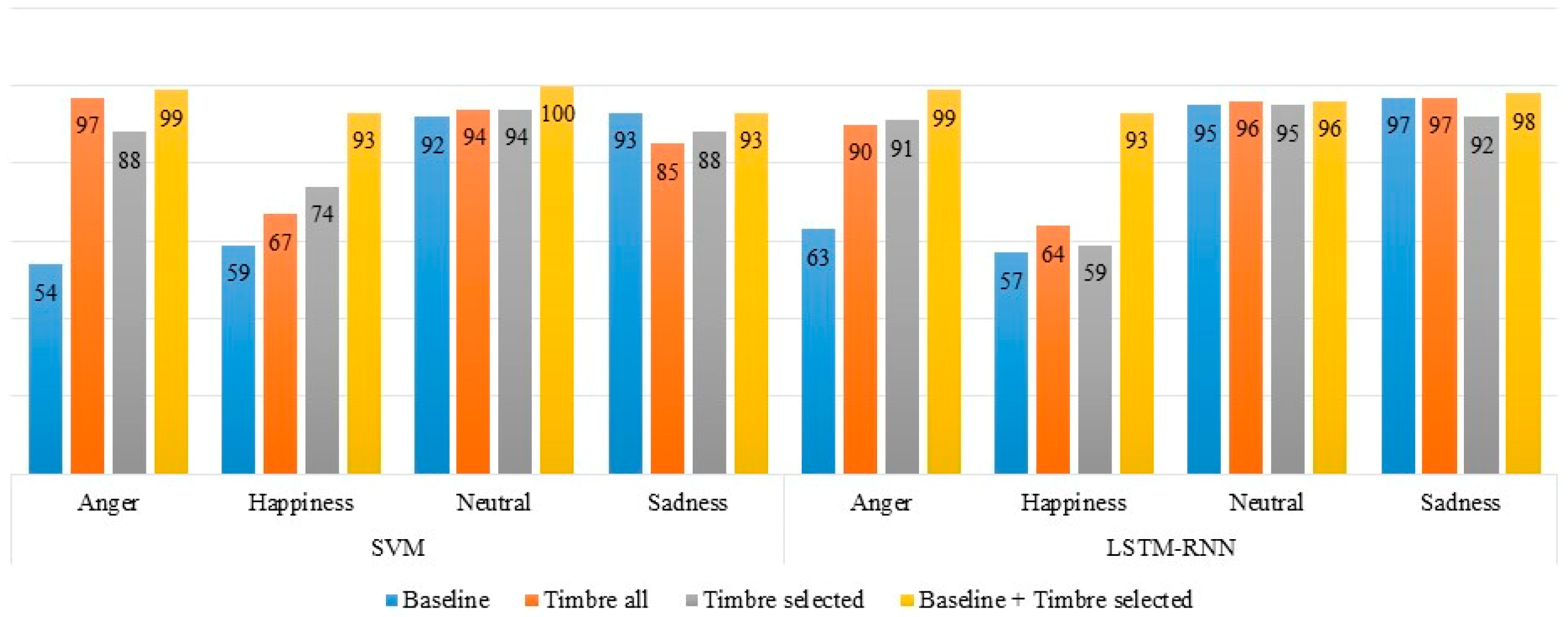
Figure 4 shows the recognition rates of positive and negative emotions obtained using all feature sets for binary classification. The recognition rates of both positive and negative emotions improved for the combination of the baseline and timbre selected feature set compared to the rest of feature sets on both SVM and LSTM-RNN. Figure 5 shows the recognition rates of discrete emotions obtained using SVM and LSTM-RNN for different acoustic feature sets. It is clear from Figure 5 that the recognition rates for all emotions were significantly better for the combination of the baseline and timbre selected acoustic feature sets compared to the recognition rates for the rest of the acoustic feature sets. The recognition rates for angry and happy emotions increased substantially for the timbre all acoustic feature set, but the changes in the results for neutral and sad emotions were not significant. Timbre features improved the discrimination of emotions that have the same level of pitch and loudness. Baseline acoustic features can discriminate emotions when the acoustic features of emotions in speech, such as pitch and loudness, are different. In

Table 6. Comparison of the results in literature with the proposed acoustic feature set for EMO-DB.

Literature	Acoustic Features	Classifier	Highest Accuracy	Database	Number of Emotions
Discrete Emotions
Quan et al. (2017) [58]	Correlation, cepstral distance, MFCC, prosodic	SVM	<80%	EMO-DB	3,4,6
Palo et al. (2018) [33]	LPCCVQC	MLP	83%	EMO-DB	4
	MFCCVQC	RBFN	79%
	PLPVQC	PNN, DNN	76%
Proposed	Baseline + timbre selected	SVM, LSTM-RNN	96.49%	EMO-DB	4
Binary Valence
Eyben et al. (2016) [5]	eGeMAPS	SVM	78.1%	EMO-DB	2
	ComParE		86.7%
proposed	Baseline + timbre selected	SVM, LSTM-RNN	97.87%	EMO-DB	2

, comparison of the results in the literature with a proposed feature set was given for EMO-DB. From Table 6, it can be seen that the proposed feature set increased recognition accuracy for both the discrete emotions classification and the binary valence classification.

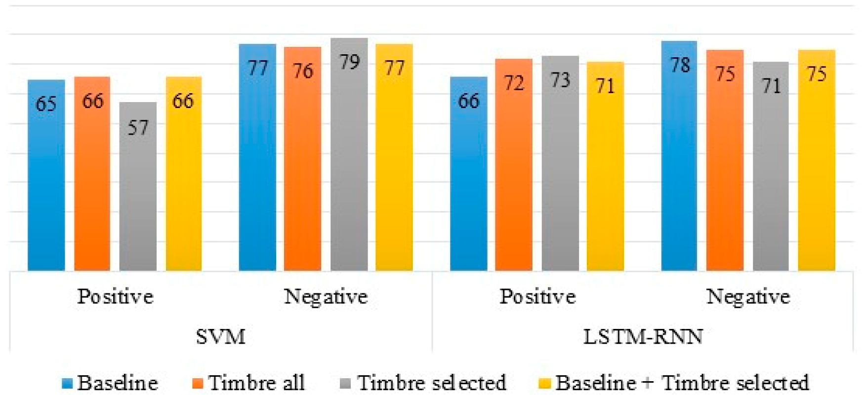
The results on IEMOCAP were different from EMO-DB. As can be seen from Table 5, the highest recognition rates for binary valence classification (74%) and the classification of discrete emotions (65.06%) were achieved using the timbre all acoustic feature set. The results obtained using the timbre selected acoustic feature set were higher than the baseline feature set and close to the timbre all feature set. Although the recognition rates on a combination of the baseline and the timbre selected feature set were better than the baseline feature set, they were lower than the results on the timbre all feature set. The baseline and timbre selected feature sets complemented each other on the IEMOCAP database. Figure 6 shows the recognition rates of positive and negative emotions achieved using the baseline, timbre all, timbre selected, and the combination of baseline and timbre selected feature sets for binary valence classification.

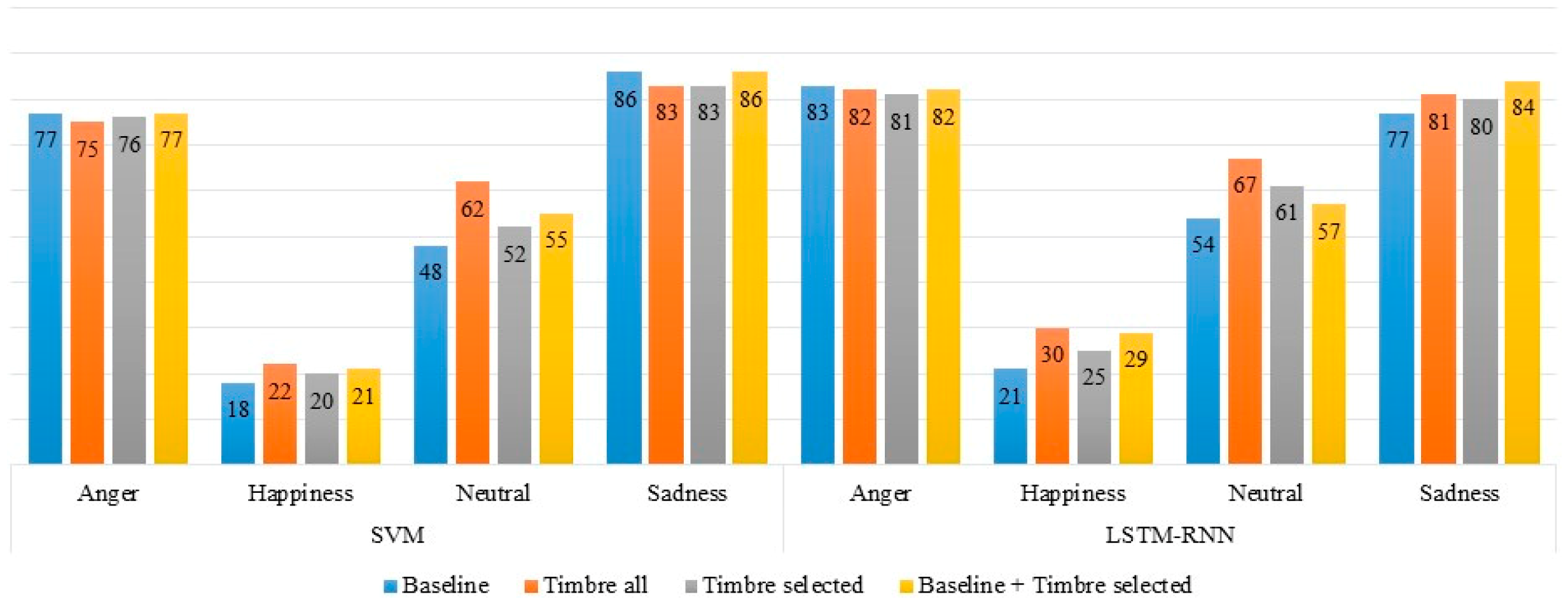
The highest recognition rate for positive emotion was obtained using the timbre all feature set increased the recognition rate of positive emotion, but it decreased for the timbre selected feature set when using SVM. The difference between recognition rates of negative emotion in all feature sets was not significant. Figure 7 presents the recognition rates of anger, happiness, neutrality, and sadness obtained using all feature sets. It is clear from Figure 7 that the timbre all feature set improved the recognition rate of all emotions except anger compared to the baseline feature set. In both classifiers, the recognition rate of emotions decreased with the timbre selected feature set compared to the timbre all feature set.

Table 7. Comparison of the results in the literature with the proposed acoustic feature set for IEMOCAP.

Literature	Acoustic Features	Classifier	Highest Accuracy	Database	Number of Emotions
Discrete emotions
Lee et al. (2015) [59]	LLDs	BLSTM-ELM	63.89%	IEMOCAP	4
Mirsamadi et al. (2017) [39]	LLDs	BLSTM-WPA	58.8%	IEMOCAP	4
Fayek et al. (2017) [45]	Spectrogram	LSTM	58.05%	IEMOCAP	4
Tzinis et al. (2017) [38]	Statistical	LSTM	60.02%	IEMOCAP	4
Proposed	Timbre all	LSTM-RNN	65.06%	IEMOCAP	4

Bidirectional LSTM with extreme learning machine (BLSTM-ELM) and weighted pooling attention (BLSTM-WPA).

shows the comparison of the results in literature with the proposed acoustic feature set for IEMOCAP. It is clear from Table 7 that the accuracy obtained using the timbre all feature set is higher than the other results in the literature. Acoustic features used in the literature is given in

Table 8. Acoustic features used in the literature [38].

Low Level Descriptors (LLDs)	Statistical Features
Root mean square (RMS) Energy	Position max/min
Quality of Voice	Arithmetic mean, standard deviation
Zero crossing rate	Skewness
Jitter Local	Kurtosis
Jitter DDP (difference of periods)	Linear regression coefficient 1/2
Shimmer Local	Quadratic & Absolute linear regression error
F0 by Sub-Harmonic sum (SHS)	Quartile 1/2/3
Loudness	Quartile range 2-1/3-2/3-1
Probability of Voicing	Percentile 99
Harmonics to noise ratio (HNR) by Autocorrelation function (ACF)	Up-level time 75/90
MFCC	Percentile 1
Line spectral pairs (LSP) Frequency	Percentile range 1–99
Log mel frequency band (MFB)	Onsets number
F0 Envelope	Duration

.

During the experiments that applied the SFS method, it was found that some of the spectral shapes (spectral skewness, kurtosis, slope, decrease, roll-off, flatness) and harmonic (harmonic energy, noise energy, harmonic spectral deviation, and odd-to-even harmonic ratio) features of timbre were all unable to characterize the emotions from speech as well as the features in the timbre that had been selected for the EMO-DB. In addition, the timbre selected consisted of only nine acoustic features, which was very useful in terms of dimensionality compared to a large-scale brute-force acoustic feature set for building an automatic SER system. Furthermore, it can characterize emotions in the valence dimension. For the EMO-DB, overall, the SVM and the LSTM-RNN gave good results for the combination of the baseline and timbre selected acoustic feature sets.

The timbre features also improved the recognition rates of emotions for the IEMOCAP. The improvement was not as high as for EMO-DB. The IEMOCAP database was originally designed to research emotion recognition from multiple modalities, including facial expressions, gesture, and speech. We only used speech to recognize the emotions, and this might not have been enough to achieve higher results for this database. However, the results are comparable to the literature results. We achieved higher results using the LSTM-RNN in terms of classifiers.

The experimental results in this work showed the effectiveness of the timbre features, which consisted of spectral and harmonic features. Timbre features can characterize emotions that share similar acoustic contents in the arousal dimension, but are different in the valence dimensions, such as anger and happiness. Moreover, we investigated whether timbre features can be used not only to discriminate instrument sounds, music emotion recognition [17,18], and music mood classification [20], but also to classify emotions in a speech signals. Spectral shape and harmonic features complement each other to describe the voice quality of a sound. When we combined timbre selected and baseline acoustic features, the results improved significantly compared to the rest of the acoustic feature sets for EMO-DB. The difference between the results of timbre and the combination of the baseline and timbre selected acoustic feature sets was not high (around 3%) for IEMOCAP. Timbre selected and the baseline acoustic features complement each other for both databases.

6. Conclusions

The primary objective of this work was to analyze the timbral acoustic features to improve the classification accuracy of emotions in the valence dimension. To accomplish this, timbre acoustic features that consisted of spectral shape and harmonic features were extracted using a timbre toolbox [30]. To find the best feature subset among the timbre acoustic features, the SFS was applied. MFCC, energy, and their first-order derivatives were also analyzed in order to compare the results. All acoustic features were divided into four groups, namely baseline (MFCC, energy and their first-order derivatives), timbre all, timbre selected and a combination of baseline and timbre selected acoustic features.

The classification was performed for binary valence and classification of categorical emotions using SVM and LSTM-RNN on the EMO-DB and IEMOCAP emotional speech databases. The average accuracy rates of 24.06% and 18.77% were improved for binary valence and discrete emotions as compared to the results using the baseline acoustic features for the EMO-DB. Although the improvement of the average classification rate for the IEMOCAP database was not high, the classification accuracy of happy and neutral emotions was improved considerably using timbre all acoustic features. The LSTM-RNN gave better results than SVM for the IEMOCAP.

In conclusion, timbre features showed their effectiveness in the classification of positive and negative emotions, as well as the classification accuracy of happy emotion improved considerably. For future work, timbre features should be analyzed for classification of fear and boredom emotions, which are also a challenge to discriminate. Moreover, timbre features need to be analyzed with other types of acoustic features to find an acoustic feature that complements timbre features.

References

1. Gunes, H.; Pantic, M. Automatic, dimensional and continuous emotion recognition. Int. J. Synth. Emot. 2010, 1, 68–99. [Google Scholar] [CrossRef]
2. Gunes, H.; Schuller, B.; Pantic, M.; Cowie, R. Emotion representation, analysis and synthesis in continuous space: A survey. In Proceedings of the Face and Gesture 2011, Santa Barbara, CA, USA, 21–25 March 2011; pp. 827–834. [Google Scholar]
3. Ciabattoni, L.; Frontoni, E.; Liciotti, D.; Paolanti, M.; Romeo, L. A sensor fusion approach for measuring emotional customer experience in an intelligent retail environment. In Proceedings of the 2017 IEEE 7th International Conference on Consumer Electronics-Berlin (ICCE-Berlin), Berlin, Germany, 3–6 September 2017; pp. 67–68. [Google Scholar]
4. Ciabattoni, L.; Ferracuti, F.; Longhi, S.; Pepa, L.; Romeo, L.; Verdini, F. Real-time mental stress detection based on smartwatch. In Proceedings of the 2017 IEEE International Conference on Consumer Electronics (ICCE), Las Vegas, NV, USA, 8–11 January 2017; pp. 110–111. [Google Scholar]
5. Eyben, F.; Scherer, K.R.; Schuller, B.W.; Sundberg, J.; André, E.; Busso, C.; Devillers, L.Y.; Epps, J.; Laukka, P.; Narayanan, S.S.; et al. The Geneva Minimalistic Acoustic Parameter Set (GeMAPS) for Voice Research and Affective Computing. IEEE Trans. Affect. Comput. 2016, 7, 190–202. [Google Scholar] [CrossRef]
6. Grimm, M.; Kroschel, K.; Mower, E.; Narayanan, S. Primitives-based evaluation and estimation of emotions in speech. Speech Commun. 2007, 49, 787–800. [Google Scholar] [CrossRef] [Green Version]
7. Grimm, M.; Kroschel, K.; Narayanan, S. Support Vector Regression for Automatic Recognition of Spontaneous Emotions in Speech. In Proceedings of the 2007 IEEE International Conference on Acoustics, Speech and Signal Processing—ICASSP ‘07, Honolulu, HI, USA, 15–20 April 2007; pp. IV-1085–IV-1088. [Google Scholar]
8. Wöllmer, M.; Eyben, F.; Reiter, S.; Schuller, B.; Cox, C.; Douglas-Cowie, E.; Cowie, R. Abandoning Emotion Classes-Towards Continuous Emotion Recognition with Modelling of Long-Range Dependencies. In Proceedings of the Interspeech 2008 9th Annual Conference of the International Speech Communication Association, Brisbane, Australia, 22–26 September 2008; pp. 597–600. [Google Scholar]
9. Juslin, P.N.; Laukka, P. Communication of emotions in vocal expression and music performance: Different channels, same code? Psychol. Bull. 2003, 129, 770. [Google Scholar] [CrossRef]
10. Lugger, M.; Yang, B. The Relevance of Voice Quality Features in Speaker Independent Emotion Recognition. In Proceedings of the 2007 IEEE International Conference on Acoustics, Speech and Signal Processing—ICASSP ‘07, Honolulu, HI, USA, 15–20 April 2007; pp. IV-17–IV-20. [Google Scholar]
11. Kim, J.; Lee, S.; Narayanan, S.S. An exploratory study of manifolds of emotional speech. In Proceedings of the 2010 IEEE International Conference on Acoustics, Speech and Signal Processing, Dallas, TX, USA, 14–19 March 2010; pp. 5142–5145. [Google Scholar]
12. Jeon, J.H.; Xia, R.; Liu, Y. Sentence level emotion recognition based on decisions from subsentence segments. In Proceedings of the 2011 IEEE International Conference on Acoustics, Speech and Signal Processing (ICASSP), Prague, Czech Republic, 22–27 May 2011; pp. 4940–4943. [Google Scholar]
13. Busso, C.; Rahman, T. Unveiling the acoustic properties that describe the valence dimension. In Proceedings of the Thirteenth Annual Conference of the International Speech Communication Association, Portland, OR, USA, 9–13 September 2012; pp. 1179–1182. [Google Scholar]
14. Goudbeek, M.; Goldman, J.P.; Scherer, K.R. Emotion Dimensions and Formant Position. In Proceedings of the Tenth Annual Conference of the International Speech Communication Association, Dresden, Germany, 6–10 September 2015; pp. 1575–1578. [Google Scholar]
15. McAdams, S.; Giordano, B.L. The perception of musical timbre. In Oxford Handbook of Music Psychology; Oxford University Press: Oxford, UK, 2009; pp. 72–80. [Google Scholar]
16. Wikipedia: The Free Encyclopedia. Available online: https://en.wikipedia.org/wiki/Timbre (accessed on 13 August 2018).
17. Klügel, N.; Groh, G. Towards Mapping Timbre to Emotional Affect. In Proceedings of the NIME, Seoul, Korea Republic, 27–30 May 2013; pp. 525–530. [Google Scholar]
18. Chau, C.-J.; Wu, B.; Horner, A. The emotional characteristics and timbre of nonsustaining instrument sounds. J. Audio Eng. Soc. 2015, 63, 228–244. [Google Scholar] [CrossRef]
19. De Leon, F.; Martinez, K. Using timbre models for audio classification. Submiss. Audio Classif. Tasks Mirex 2013, 2013. Available online: http://citeseerx.ist.psu.edu/viewdoc/download?doi=10.1.1.415.7285&rep=rep1&type=pdf (accessed on 15 September 2018).
20. Ren, J.-M.; Wu, M.-J.; Jang, J.-S.R. Automatic music mood classification based on timbre and modulation features. IEEE Trans. Affect. Comput. 2015, 6, 236–246. [Google Scholar] [CrossRef]
21. Goudbeek, M.; Scherer, K. Beyond arousal: Valence and potency/control cues in the vocal expression of emotion. J. Acoust. Soc. Am. 2010, 128, 1322–1336. [Google Scholar] [CrossRef] [PubMed]
22. Eyben, F.; Weninger, F.; Schuller, B. Affect recognition in real-life acoustic conditions-A new perspective on feature selection. In Proceedings of the Interspeech 2013 14th Annual Conference of the International Speech Communication Association, Lyon, France, 25–29 August 2013. [Google Scholar]
23. Tamarit, L.; Goudbeek, M.; Scherer, K. Spectral slope measurements in emotionally expressive speech. In Proceedings of the Speech Analysis and Processing for Knowledge Discovery, Aalborg, Denmark, 4–6 June 2008; pp. 169–183. [Google Scholar]
24. Le, P.N.; Ambikairajah, E.; Epps, J.; Sethu, V.; Choi, E.H. Investigation of spectral centroid features for cognitive load classification. Speech Commun. 2011, 53, 540–551. [Google Scholar] [CrossRef]
25. Schuller, B.; Weninger, F.; Zhang, Y.; Ringeval, F.; Batliner, A.; Steidl, S.; Eyben, F.; Marchi, E.; Vinciarelli, A.; Scherer, K. Affective and behavioural computing: Lessons learnt from the first computational paralinguistics challenge. Comput. Speech Lang. 2019, 53, 156–180. [Google Scholar] [CrossRef]
26. Yildirim, S.; Bulut, M.; Lee, C.M.; Kazemzadeh, A.; Deng, Z.; Lee, S.; Narayanan, S.; Busso, C. An acoustic study of emotions expressed in speech. In Proceedings of the Eighth International Conference on Spoken Language Processing, Jeju Island, Korea, 4–8 October 2004; pp. 2193–2196. [Google Scholar]
27. Zhao, J.; Mao, X.; Chen, L. Learning deep features to recognise speech emotion using merged deep CNN. IET Signal. Process. 2018, 12, 713–721. [Google Scholar] [CrossRef]
28. Fayek, H.M.; Lech, M.; Cavedon, L. Towards real-time speech emotion recognition using deep neural networks. In Proceedings of the 2015 9th International Conference on Signal Processing and Communication Systems (ICSPCS), Cairns, Australia, 14–16 December 2015; pp. 1–5. [Google Scholar]
29. Zhang, Z.; Wu, B.; Schuller, B. Attention-augmented End-to-end Multi-task Learning for Emotion Prediction from Speech. In Proceedings of the 2019 IEEE International Conference on Acoustics, Speech and Signal Processing (ICASSP), Brighton, UK, 12–17 May 2019; pp. 6705–6709. [Google Scholar]
30. Peeters, G.; Giordano, B.L.; Susini, P.; Misdariis, N.; McAdams, S. The Timbre Toolbox: Extracting audio descriptors from musical signals. J. Acoust. Soc. Am. 2011, 130, 2902–2916. [Google Scholar] [CrossRef] [PubMed] [Green Version]
31. Singh, P.P.; Rani, P. An approach to extract feature using mfcc. IOSR J. Eng. 2014, 4, 21–25. [Google Scholar] [CrossRef]
32. Cao, H.; Verma, R.; Nenkova, A. Speaker-sensitive emotion recognition via ranking: Studies on acted and spontaneous speech. Comput. Speech Lang. 2015, 29, 186–202. [Google Scholar] [CrossRef] [PubMed]
33. Palo, H.; Mohanty, M.N. Comparative Analysis of Neural Networks for Speech Emotion Recognition. Int. J. Eng. Technol. 2018, 7, 112–116. [Google Scholar]
34. Nwe, T.L.; Foo, S.W.; De Silva, L.C. Speech emotion recognition using hidden Markov models. Speech Commun. 2003, 41, 603–623. [Google Scholar] [CrossRef]
35. Shrawankar, U.; Thakare, V.M. Techniques for feature extraction in speech recognition system: A comparative study. Int. J. Comput. Appl. Eng. Technol. Sci. 2013, 1145, 412–418. [Google Scholar]
36. Koolagudi, S.G.; Rao, K.S. Emotion recognition from speech: A review. Int. J. Speech Technol. 2012, 15, 99–117. [Google Scholar] [CrossRef]
37. Chapelle, O.; Vapnik, V. Model selection for support vector machines. In Advances in Neural Information Processing Systems; MIT Press: Cambridge, MA, USA, 2000; pp. 230–236. [Google Scholar]
38. Tzinis, E.; Potamianos, A. Segment-based speech emotion recognition using recurrent neural networks. In Proceedings of the 2017 Seventh International Conference on Affective Computing and Intelligent Interaction (ACII), San Antonio, TX, USA, 23–26 October 2017; pp. 190–195. [Google Scholar]
39. Mirsamadi, S.; Barsoum, E.; Zhang, C. Automatic speech emotion recognition using recurrent neural networks with local attention. In Proceedings of the 2017 IEEE International Conference on Acoustics, Speech and Signal Processing (ICASSP), New Orleans, LA, USA, 5–9 March 2017; pp. 2227–2231. [Google Scholar]
40. Graves, A.; Mohamed, A.-r.; Hinton, G. Speech recognition with deep recurrent neural networks. In Proceedings of the 2013 IEEE International Conference on Acoustics, Speech and Signal Processing (ICASSP), Vancouver, Canada, 26–30 May 2013; pp. 6645–6649. [Google Scholar]
41. Eyben, F.; Weninger, F.; Squartini, S.; Schuller, B. Real-life voice activity detection with LSTM Recurrent Neural Networks and an application to Hollywood movies. In Proceedings of the 2013 IEEE International Conference on Acoustics, Speech and Signal Processing (ICASSP), Vancouver, Canada, 26–30 May 2013; pp. 483–487. [Google Scholar]
42. Graves, A.; Jaitly, N. Towards end-to-end speech recognition with recurrent neural networks. In Proceedings of the International Conference on Machine Learning, Beijing, China, 21–26 June 2014; pp. 1764–1772. [Google Scholar]
43. Fonnegra, R.D.; Díaz, G.M. Speech Emotion Recognition Based on a Recurrent Neural Network Classification Model. In Proceedings of the International Conference on Advances in Computer Entertainment, London, UK, 14–16 December 2017; pp. 882–892. [Google Scholar]
44. Hochreiter, S.; Schmidhuber, J. Long short-term memory. Neural Comput. 1997, 9, 1735–1780. [Google Scholar] [CrossRef]
45. Fayek, H.M.; Lech, M.; Cavedon, L. Evaluating deep learning architectures for Speech Emotion Recognition. Neural Netw. 2017, 92, 60–68. [Google Scholar] [CrossRef]
46. Huang, K.-Y.; Wu, C.-H.; Hong, Q.-B.; Su, M.-H.; Chen, Y.-H. Speech Emotion Recognition Using Deep Neural Network Considering Verbal and Nonverbal Speech Sounds. In Proceedings of the 2019 IEEE International Conference on Acoustics, Speech and Signal Processing (ICASSP), Brighton, UK, 12–17 May 2019; pp. 5866–5870. [Google Scholar]
47. Burkhardt, F.; Paeschke, A.; Rolfes, M.; Sendlmeier, W.F.; Weiss, B. A database of German emotional speech. In Proceedings of the Ninth European Conference on Speech Communication and Technology, Lisboa, Portugal, 4–8 September 2005; pp. 1517–1520. [Google Scholar]
48. Gangamohan, P.; Kadiri, S.R.; Gangashetty, S.V.; Yegnanarayana, B. Excitation source features for discrimination of anger and happy emotions. In Proceedings of the Fifteenth Annual Conference of the International Speech Communication Association, Singapore, 14–18 September 2014; pp. 1253–1257. [Google Scholar]
49. Kadiri, S.R.; Gangamohan, P.; Gangashetty, S.V.; Yegnanarayana, B. Analysis of excitation source features of speech for emotion recognition. In Proceedings of the Sixteenth Annual Conference of the International Speech Communication Association, Dresden, Germany, 6–10 September 2015; pp. 1324–1328. [Google Scholar]
50. Busso, C.; Bulut, M.; Lee, C.-C.; Kazemzadeh, A.; Mower, E.; Kim, S.; Chang, J.N.; Lee, S.; Narayanan, S.S. IEMOCAP: Interactive emotional dyadic motion capture database. Lang. Resour. Eval. 2008, 42, 335. [Google Scholar] [CrossRef]
51. Eyben, F.; Wöllmer, M.; Schuller, B. Opensmile: The munich versatile and fast open-source audio feature extractor. In Proceedings of the 18th ACM international conference on Multimedia, Boston, MA, USA, 18–22 November 1996; pp. 1459–1462. [Google Scholar]
52. Rao, K.S.; Koolagudi, S.G. Robust emotion recognition using pitch synchronous and sub-syllabic spectral features. In Robust Emotion Recognition Using Spectral and Prosodic Features; Springer: Berlin/Heidelberg, Germany, 2013; pp. 17–46. [Google Scholar]
53. Kamińska, D.; Sapiński, T.; Pelikant, A. Comparison of perceptual features efficiency for automatic identification of emotional states from speech. In Proceedings of the 2013 6th International Conference on Human System Interactions (HSI), Gdansk, Poland, 6–8 June 2013; pp. 210–213. [Google Scholar]
54. Yuan, J.; Chen, L.; Fan, T.; Jia, J. Dimension reduction of speech emotion feature based on weighted linear discriminate analysis. Image Process. Pattern Recognit. 2015, 8, 299–308. [Google Scholar]
55. Spence, C.D.; Sajda, P. Role of feature selection in building pattern recognizers for computer-aided diagnosis. In Proceedings of the Medical Imaging 1998: Image Processing, San Diego, CA, USA, 21–26 February 1998; pp. 1434–1442. [Google Scholar]
56. Keras: The Python Deep Learning library. Available online: https://keras.io/ (accessed on 17 April 2018).
57. Badshah, A.M.; Rahim, N.; Ullah, N.; Ahmad, J.; Muhammad, K.; Lee, M.Y.; Kwon, S.; Baik, S.W. Deep features-based speech emotion recognition for smart affective services. Multimed. Tools Appl. 2017, 78, 5571–5589. [Google Scholar] [CrossRef]
58. Quan, C.; Zhang, B.; Sun, X.; Ren, F. A combined cepstral distance method for emotional speech recognition. Int. J. Adv. Robot. Syst. 2017, 14, 172–184. [Google Scholar] [CrossRef]
59. Lee, J.; Tashev, I. High-level feature representation using recurrent neural network for speech emotion recognition. In Proceedings of the Sixteenth Annual Conference of the International Speech Communication Association, Dresden, Germany, 6–10 September 2015. [Google Scholar]
Figure 1. Representation of seven basic emotions in the arousal-valence dimension.
Applsci 09 02470 g001
Figure 2. General speech emotion recognition system.
Applsci 09 02470 g002
Figure 3. Complete MFCC feature extraction process.
Applsci 09 02470 g003
Figure 4. Recognition rates of positive and negative emotions on baseline, timbre all, timbre selected, and the combination of baseline and timbre selected acoustic feature sets for EMO-DB.
Applsci 09 02470 g004
Figure 5. Recognition rates for discrete emotions on baseline, timbre all, timbre selected, and the combination of baseline and timbre selected acoustic features for EMO-DB.
Applsci 09 02470 g005
Figure 6. Recognition rates of positive and negative emotions on baseline, timbre all, timbre selected, and the combination of baseline and timbre selected acoustic feature sets for IEMOCAP.
Applsci 09 02470 g006
Figure 7. Recognition rates of discrete emotions on baseline, timbre all, timbre selected, and the combination of baseline and timbre selected acoustic features for IEMOCAP.
Applsci 09 02470 g007