Numerical–Experimental Correlation of Impact-Induced Damages in CFRP Laminates

Featured Application

Numerical investigation on the damage behavior of CFRP laminates subjected to low velocity impacts.

Abstract

Composite laminates are characterized by high mechanical in-plane properties and poor out-of-plane characteristics. This issue becomes even more relevant when dealing with impact phenomena occurring in the transverse direction. In aeronautics, Low Velocity Impacts (LVIs) may occur during the service life of the aircraft. LVI may produce damage inside the laminate, which are not easily detectable and can seriously degrade the mechanical properties of the structure. In this paper, a numerical-experimental investigation is carried out, in order to study the mechanical behavior of rectangular laminated specimens subjected to low velocity impacts. The numerical model that best represents the impact phenomenon has been chosen by numerical–analytical investigations. A user defined material model (VUMAT) has been developed in Abaqus/Explicit environment to simulate the composite intra-laminar damage behavior in solid elements. The analyses results were compared to experimental test data on a laminated specimen, performed according to ASTM D7136 standard, in order to verify the robustness of the adopted numerical model and the influence of modeling parameters on the accuracy of numerical results.

1. Introduction

Composite materials are characterized by high mechanical properties values if compared to classic metallic materials. However, their damage behavior is difficult to predict and control. As a matter of fact, impact events on a composite structure are still a “hot topic” for research, nowadays. The different impact phenomena can be divided into three main groups, based on the velocity of the impactor: low velocity impacts, ballistic impacts, and hyper-velocity impacts. In particular, Low Velocity Impacts (LVIs) often result in Barely Visible Impact Damages (BVIDs), which can be hardly detected by the naked eye, but may relevantly decrease the material strength [1,2,3]. Damages occurring as a consequence of low velocity impacts include both intra-laminar (fiber and/or matrix failure) and inter-laminar damages (delaminations). Among the others, delaminations, which can growth under service loads, can seriously reduce the load carrying capability of the overall structure [4,5]. For this reason, a large number of studies, focused on the prediction of the damages (especially delaminations) induced by LVI, can be found in the literature. In these studies, different approaches, both analytical–numerical and experimental, were considered [6,7,8,9]. Different techniques are available and presented in the literature, able to predict and evaluate the damage and the residual strength during LVI phenomena. In [10], an acousto–ultrasonic approach was used to characterize the material impact strength. Low velocity analytical impact prediction models available in the literature are often characterized by a large degree of simplification. However, despite the simplifications in the models, good results can be achieved. In particular, the study in Reference [11] describes a numerical model for predicting the onset and the propagation of damages arising from low velocity impacts induced by large and small impact masses. A further evolution of the analytical model for predicting the behavior of a thin-walled composite structure during a low velocity-high mass impact phenomenon was presented in [12]. An additional analytical methodology based on the energy balance for the development of damage during a LVI phenomenon with the help of a localized strain field was introduced in [13]. However, analytical approaches, which can only be adopted for few particular conditions [1,6,7], cannot be generally considered for a complete and detailed study of the impact event, due to inherent complexity of the impact phenomenon itself [9,14,15,16]. A more comprehensive study of the impact phenomenon can be surely obtained by means of numerical methods. Indeed, FEM (Finite Element Method) codes can be adopted to model a low velocity impact event on a composite specimen, taking into account both intra-laminar and inter-laminar damages [9,17,18,19]. In order to evaluate the intra-laminar and inter-laminar damage onset and propagation during an impact phenomenon, progressive damage methods have been presented by several authors, showing good results compared to the experimental data. In [20], LVI tests were performed and the Puck criteria were adopted to analyze the composite structure mechanical response. In the same work, an inter-laminar matrix crack density parameter was introduced, in order to mitigate the computational cost, while decreasing, on the other side, the analysis accuracy. In [21,22,23], a model capable of predicting the inter-laminar damage in a unidirectional composite laminate was introduced. In particular, the proposed model took into account a matrix non-linear shear behavior, focusing on the element characteristic length in order to alleviate the mesh dependency. Actually, fracture mechanic is widely used to model inter-laminar damage evolution through FE-based procedures such as Virtual Crack Closure Technique (VCCT) and Cohesive Zone Model theory (CZM) [17,24,25,26,27,28,29]. In [29,30,31], the influence of intra-laminar damages on the inter-laminar ones is assessed adopting CZM, while, in [26,31,32,33], the mesh-dependency issue of both inter-laminar and intra-laminar prediction models, which may lead to an unrealistic inter-laminar damage prediction, is emphasized. Low velocity impact events on composite specimens, with different stacking sequences, were studied in several works, which implement the intra-laminar and inter-laminar damages, respectively, by means of Continuum Damage Mechanics (CDM) and CZM approaches [9,18,19]. In these works, good results, in terms of correlation between numerical outputs and experimental data, were obtained for various impact energy levels.

In this work, we propose an analytical model to preliminary evaluate the response of a unidirectional composite plate subjected to a low velocity impact. The analytical model has been developed in accordance with [1,2,33]. Then, the results of the analytical model were compared with those from a numerical model, which uses the analytical boundary conditions. Indeed, in the frame of this first step, the introduced analytical model, based on Classical Laminated Plate Theory (CLPT), was adopted as a benchmark for appropriately selecting the main numerical modeling parameters to be used for the numerical procedure (element type, mesh density, element size, etc.). Subsequently, the numerical model was improved, introducing the boundary conditions of the experimental test. Finally, a further numerical model, which takes into account inter-laminar and intra-laminar damages, was implemented and the results were compared with the experimental test ones. This final numerical test was performed by adopting the numerical model, from the previous step, which best represents the impact event. The low velocity impact phenomenon was numerically simulated by considering the boundary conditions and the specimen size according to the ASTM (American Society for Testing and Materials) D7136 standard [34]. The composite specimens were subjected to a 10 J low velocity impact. A reduction of the computational time has been achieved by introducing global/local techniques [35] between the impacted area and the rest of the specimen. The results, in terms of intra-laminar and inter-laminar damages, have been compared with the experimental ones, obtained by means of Ultrasonic C-Scan tests. Further numerical–experimental correlations on the impactor displacement and velocity, the internal energy, and the force exerted during the impact have been performed as well.

Numerical results, obtained considering different Abaqus element types, were compared to each other. The Finite Element Model has been discretized by means of SC8R Continuum shell elements and C3D8R Solid elements [36]. Inter-laminar damages were modeled by a Cohesive Zone Model based approach, while intra-laminar damage was modeled by means of Hashin’s failure criteria and gradual material properties degradation rules. However, the intra-laminar damage model was only provided for Continuum shell elements in Abaqus. Since no intra-laminar damage model was provided for Solid elements, a user-defined material model, able to take into account the intra-laminar damage, was implemented in a user subroutine VUMAT.

In Section 2, the theoretical background on the analytical model and on the intra-laminar damage model implemented in the VUMAT are presented. In Section 3, the test cases are introduced, while in Section 4 the results are presented and discussed.

2. Theoretical background

2.1. Classical Laminated Plate Theory

A multi-degree of freedom analytical model [1,2,37] was introduced in order to study the impact event. A simply supported plate was analytically solved by using the Classical Laminated Plate Theory. The solutions for the analytical approach were obtained in terms of contact force, maximum displacement, impactor velocity, and kinetic energy. Then, a system of ordinary differential equations (ODE), representing the simply supported plate, coupled with a differential equation representing the impactor motion, was obtained.

A laminated composite plate, with in-plane dimensions a and b, respectively, along the x- and y-directions, was considered. The plate was considered simply supported along the four edges, and a concentrated force was applied at the center (x₀ = a/2, y₀ = b/2). Under these assumptions, the equation of motion along the transverse direction can be expressed as the following system of ordinary differential equations [1]:

$${\ddot{\alpha }}_{mn}+{\omega }_{mn}^2{\alpha }_{mn}=\frac{4F}{ab{I}_1}\sin \left(\frac{m\pi x_0}{a}\right)\sin \left(\frac{n\pi y_0}{b}\right),$$

(1)

In Equation (1), F is a concentrated applied force, while ω_mn, which is the natural frequency of the system for the strain modes m,n, is given by:

$${\omega }_{mn}=\sqrt{\frac{{\pi }^4}{a^4{I}_1}\left(D_{11}{m}^4+2\left(D_{12}+2D_{66}\right)m^2{n}^2{r}^2-4D_{16}{m}^{3}nr-4D_{26}m{n}^3{r}^3+D_{22}{n}^4{r}^4\right)},$$

(2)

where D_ij are the terms of the bending stiffness matrix, I₁ is the mass per unit length, and r = a/b.

As reported in [1], when both values of m and n are negative, the effects of deflection in the plate become negligible. The choice of high positive values for both values is related to the phenomenon being analyzed: as the values of m and n increase, the rotary inertia and shear deformation effects becomes significant.

Moreover, the following Equation (3), governing the impactor dynamic, has been considered:

$$M\ddot{z}\left(t\right)+F_c\left(t\right)=0,$$

(3)

where M and $\ddot{z}\left(t\right)$ are, respectively, the impactor mass and acceleration, F_c(t) is the contact force, and t is the time variable.

A proper contact law has been chosen to couple Equations (3) and (1). In particular, the contact force F_c(t) has been related to the indentation α = z(t) − w₀(x₀,y₀,t), expressed as the difference between the impactor displacement z(t) and the laminate central point displacement w₀(x₀,y₀,t). In this work, a linearized form of the Hertz Contact Law was adopted [37], therefore the contact force history, exerted during the impact phenomenon, can be expressed as:

$$F_c\left(t\right)=k_y\alpha ,$$

(4)

where k_y represents the linearized contact stiffness.

The boundary conditions of the system of ODEs are:

$${\alpha }_{mn}\left(0\right)={\dot{\alpha }}_{mn}\left(0\right)=0,$$

(5)

$$\begin{array}{l}z\left(0\right)=0\\ \dot{z}\left(0\right)=V\end{array}$$

(6)

where V is the initial velocity of the impactor.

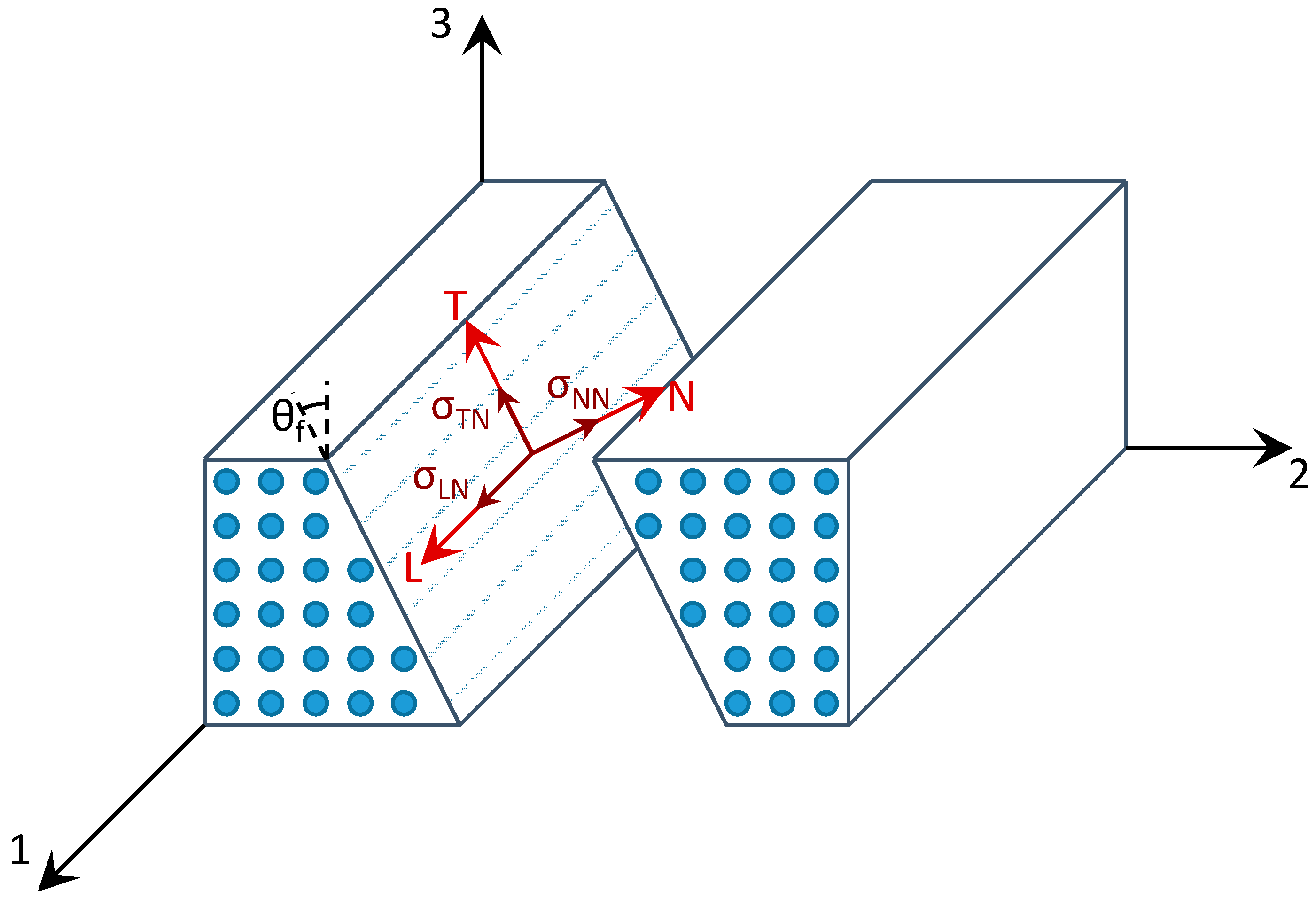
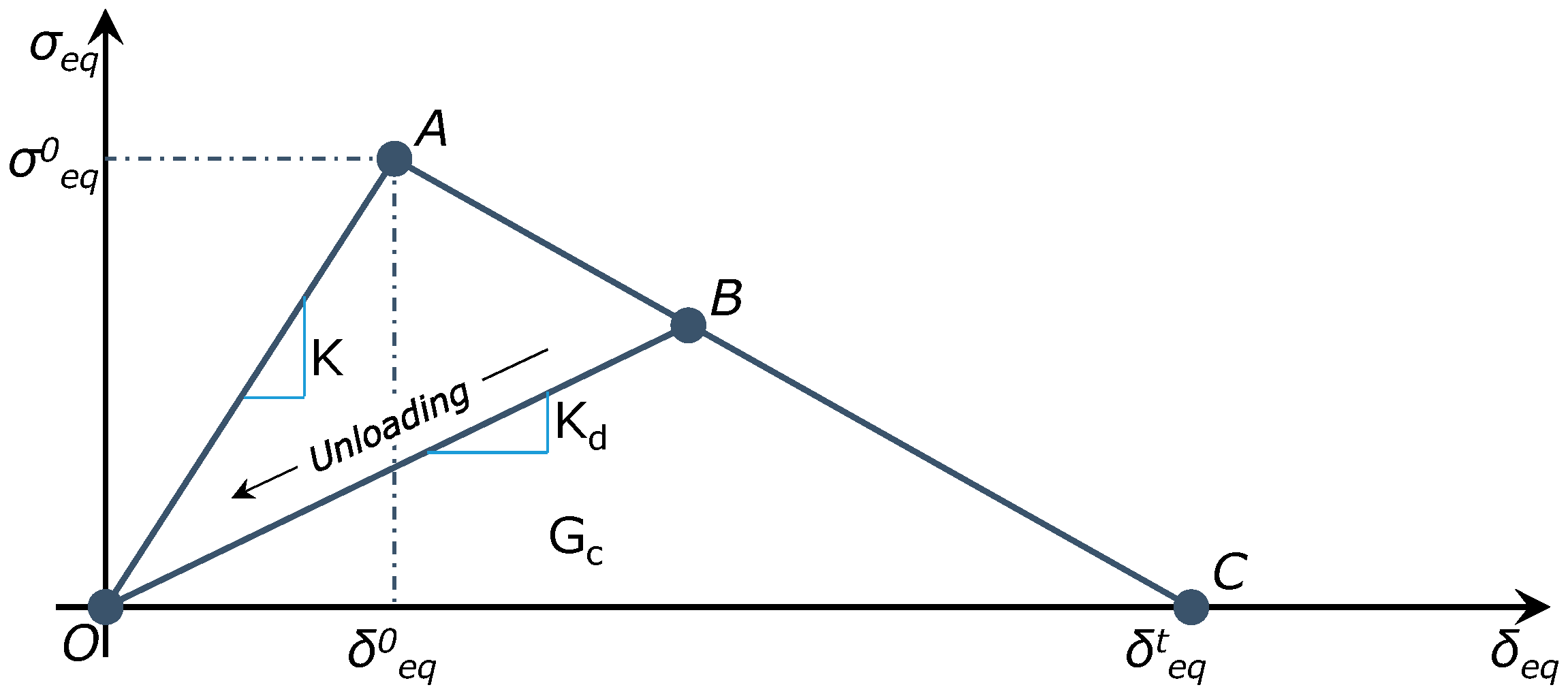
2.2. Composites Damage Criteria

In order to account for the damage behavior of the laminate, a User Material was developed in the ABAQUS FEM environment capable to consider the fiber and matrix damage mechanisms in tension and compression [4,19,29]. Each failure mode consisted of two different phases. Initially, a linear mechanical behavior is considered up to the damage initiation threshold. Then, the damage evolution up to the complete damage is evaluated.

The criteria used for evaluate the damage initiation are based on Hashin’s (fiber and matrix tension and fiber compression) and Puck–Shurmann [38] (matrix compression) failure criteria, as reported in Equations (7)–(10).

$$F_{ft}=\left(\frac{{\sigma }_1}{X_T}\right)\ge 1if{\sigma }_1\ge 0,$$

(7)

$$F_{fc}=\left(\frac{{\sigma }_1}{X_C}\right)\ge 1if{\sigma }_1<0,$$

(8)

$$F_{mt}={\left(\frac{{\sigma }_2}{Y_T}\right)}^2+{\left(\frac{{\tau }_{12}}{S_{12}}\right)}^2+{\left(\frac{{\tau }_{23}}{S_{23}}\right)}^2\ge 1if{\sigma }_2\ge 0,$$

(9)

$$F_{mc}={\left(\frac{{\tau }_{nt}}{S_{23}^A-{\mu }_{nt}{\sigma }_{nn}}\right)}^2+{\left(\frac{{\tau }_{nl}}{S_{12}-{\mu }_{nl}{\sigma }_n}\right)}^2\ge 1if{\sigma }_2<0,$$

(10)

where X_T and X_C are the fiber tensile and compressive strengths, Y_T is the matrix tensile strength, and S₁₂ and S₂₃ are respectively the longitudinal and transverse shear strengths. Moreover, the parameters introduced in Equation (10) have been defined with respect to the potential fracture plane; in particular, S^A₂₃ is the transverse shear strength in the potential fracture plane, μ_nt and μ_nl are respectively the friction coefficients in the transverse and longitudinal directions, σ_nn is the normal stress, and τ_nt and τ_nl are respectively the shear stresses in the transverse and longitudinal directions. Indeed, experiments have demonstrated that unidirectional laminates experience shear fail [39] when subjected to transverse compressive loads, with a fracture plane oriented with an angle θ_f = 53° ± 2° [21]. Hence, to correctly evaluate the damage status of the laminate, the stress/strain components in the θ_f oriented fracture plane have been considered, instead of the nominal 0° oriented nominal plane.

Therefore, the stress components in the general fracture plane L-N-T oriented with a fracture angle θ_f, as in Figure 1, can be obtained as a function of the stress components defined in the lamina coordinate system 1-2-3:

$$\{\begin{array}{l}{\sigma }_n={\sigma }_2{\cos }^2{\theta }_f+{\sigma }_3{\sin }^2{\theta }_f+2{\tau }_{23}\cos {\theta }_f\sin {\theta }_f\\ {\tau }_{nl}={\tau }_{23}\cos {\theta }_f+{\tau }_{31}\cos {\theta }_f\\ {\tau }_{nt}=\left({\sigma }_3-{\sigma }_2\right)\cos {\theta }_f\sin {\theta }_f+{\tau }_{23}\left({\cos }^2{\theta }_f-{\sin }^2{\theta }_f\right)\end{array}.$$

(11)

Hence, the parameters related to the fracture angle introduced in Equation (10) can be defined [40]:

$$\varphi =2\cdot {\theta }_f-90°,$$

(12)

$${\mu }_{nt}=\tan \varphi ,$$

(13)

$$S_{23}^A=\frac{Y_C\left(1-\sin \varphi \right)}{2\cos \varphi },$$

(14)

$${\mu }_{nl}={\mu }_{nt}\cdot \frac{S_{12}}{S_{23}^A},$$

(15)

where Y_T is the matrix compressive strength.

Each mode is characterized by the failure behavior reported in Figure 2. In particular, a linear elastic behavior with an initial stiffness K can be observed up to location A, which identifies the damage onset. Then, each location B on the segment AC identifies a partial damage condition characterized by a degraded stiffness K_d, up to location C, where the complete failure can be observed.

To take into account the material stiffness degradations in locations B, the damage coefficients d_i [36] are introduced for each failure mode:

$$d_i=\frac{{\delta }_{i,eq}^t\left({\delta }_{i,eq}-{\delta }_{i,eq}^0\right)}{{\delta }_{i,eq}\left({\delta }_{i,eq}^t-{\delta }_{i,eq}^0\right)};{\delta }_{i,eq}^0\le {\delta }_{i,eq}\le {\delta }_{i,eq}^t;i\in \left(fc,ft,mc,mt\right).$$

(16)

Indeed, the damaged stiffness matrix C_D can be expressed as a function of the damage coefficients as:

$$C_D=\frac{1}{D}\left[\begin{array}{ccc}\left(1-d_f\right)E_1& \left(1-d_f\right)\left(1-d_m\right){\nu }_{21}{E}_1& 0\\ \left(1-d_f\right)\left(1-d_m\right){\nu }_{12}{E}_2& \left(1-d_m\right)E_2& 0\\ 0& 0& D\left(1-d_s\right)G_{12}\end{array}\right],$$

(17)

where D = 1 − (1 − d_f)(1 − d_m)ν₁₂ν₂₁, and d_f, d_m, and d_s are respectively the fiber, matrix, and shear damage coefficients:

$$\begin{array}{l}{d}_f=\{\begin{array}{cc}{d}_{ft}& \mathrm{if}{\widehat{\sigma }}_{11}\ge 0\\ d_{fc}& \mathrm{if}{\widehat{\sigma }}_{11}<0\end{array}\\ d_m=\{\begin{array}{cc}{d}_{mt}& \mathrm{if}{\widehat{\sigma }}_{22}\ge 0\\ d_{mc}& \mathrm{if}{\widehat{\sigma }}_{22}<0\end{array}\\ d_s=1-\left(1-d_{ft}\right)\left(1-d_{fc}\right)\left(1-d_{mt}\right)\left(1-d_{mc}\right)\end{array}$$

(18)

However, this methodology has been found strongly dependent on the domain discretization. Hence, to reduce mesh dependencies, the element characteristic length L_C has been introduced. In this work, the solution proposed by Bazant and Oh [39] and reported in Equation (19) has been adopted:

$$L_C=\frac{\sqrt{A_{ip}}}{\cos \theta },$$

(19)

where Aip is the Area of the element corresponding to the ip-th integration point and θ is the fracture angle. Then, the equivalent displacements was computed as a function of the element characteristic length L_C:

$${\delta }_{mt,eq}^0=\frac{\sqrt{{\left({\epsilon }_2\cdot L_C\right)}^2+{\left({\gamma }_{12}\cdot L_C\right)}^2+{\left({\gamma }_{23}\cdot L_C\right)}^2}}{\sqrt{F_{mt}}},$$

(20)

$${\delta }_{mc,eq}^0=\frac{\sqrt{{\left({\gamma }_{\ln }\cdot L_C\right)}^2+{\left({\gamma }_{tn}\cdot L_C\right)}^2}}{\sqrt{F_{mc}}},$$

(21)

$${\delta }_{i,eq}^0=\frac{\sqrt{{\left({\epsilon }_1\cdot L_C\right)}^2}}{\sqrt{F_i}};i\in \left(fc,ft\right),$$

(22)

$${\delta }_{ft,eq}^t=\frac{2G_{IC}^T}{{\sigma }_{ft,eq}^0},$$

(23)

$${\delta }_{fc,eq}^t=\frac{2G_{IC}^C}{{\sigma }_{fc,eq}^0},$$

(24)

$${\delta }_{mt,eq}^t=\frac{2G_{IIC}^T}{{\sigma }_{mt,eq}^0},$$

(25)

$${\delta }_{mc,eq}^t=\frac{2G_{IIC}^C}{{\sigma }_{mc,eq}^0},$$

(26)

where G^T_IC and G^C_IC are the tensile and compressive Mode I fracture toughness, G^T_IIC and G^C_IIC are the tensile and compressive Mode II fracture toughness, and:

$${\gamma }_{nt}={\gamma }_{12}\cos {\theta }_f+{\gamma }_{13}\sin {\theta }_f,$$

(27)

$${\gamma }_{nl}=-{\epsilon }_2\cos {\theta }_f\sin {\theta }_f+{\epsilon }_3\cos {\theta }_f\sin {\theta }_f+{\gamma }_{23}\left(2{\cos }^2{\theta }_f-1\right).$$

(28)

3. Test Cases Descriptions

3.1. Analytical Set-Up

The analyzed test case is a simply supported laminated plate impacted by a 3.58 kg mass steel sphere. A 10 J impact energy is considered, leading to an impactor initial velocity equal to 2.364 m/s. The plate is made by a unidirectional carbon-fiber laminate, with in-plane dimensions in the x- and y-directions, respectively, a = 150 mm and b = 100 mm. The stacking sequence of the laminate is [45/-45/0/0/90/0]_2S, while the mechanical properties of the adopted material system and the ply thickness are reported in

Table 1. Lamina mechanical properties.

Property [unit]	Value
ρ [kg/m3]	1600
E11 [MPa]	149,500
E22 = E33 [MPa]	8430
G12 = G13 [MPa]	4200
G23 [MPa]	2520
υ12 = υ13 [-]	0.3
υ23 [-]	0.45
υ21 [-]	0.0186
XT [MPa]	2143
XC [MPa]	1034
YT [MPa]	75
YC [MPa]	250
S12 = S13 [MPa]	108
S23 [MPa]	95
GT1c [kJ/m2]	30.72
GC1c [kJ/m2]	7.15
GT2c [kJ/m2]	0.667
GC2c [kJ/m2]	7.41
Ply thickness [mm]	0.186

.

A spherical impactor with an 8 mm in radius was considered. The linear contact stiffness was set equal to k_y = 7.8755 × 10³ N/mm, according to the equations reported in [34]. In these analyses, aimed to preliminary assess the elastic behavior of the structure under impact loading conditions, only the elastic behavior has been taken into account. Therefore, no damage has been considered.

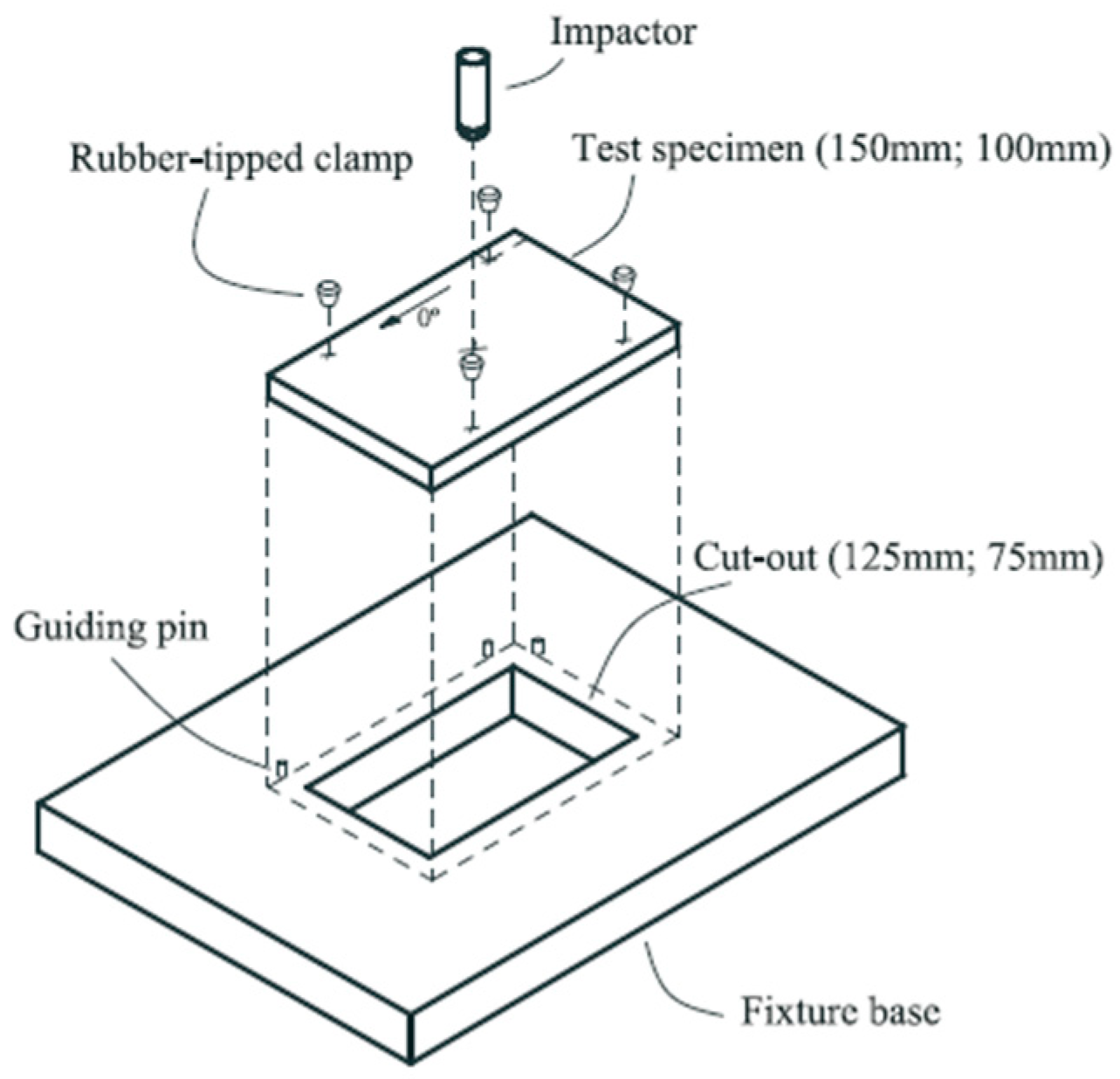
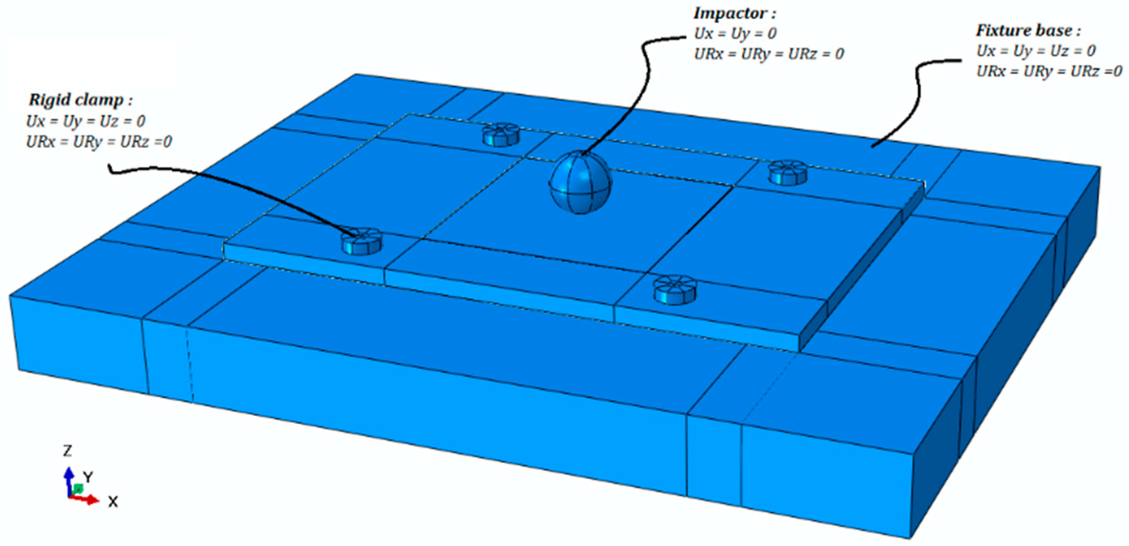
3.2. Experimental Set-Up

The experimental impact test was performed according to the ASTM D7136 standard [34], as shown in Figure 3.

The three tested specimens were cut from a single CFRP plate by using the waterjet technique. The CFRP plate is composed of prepreg high modulus carbon fiber and thermoset epoxy resin, cured in autoclave. The test was performed with the CEAST Fractovis plus drop tower test machine. The plates were normally impacted at the center. The impactor was a 16 mm diameter hemisphere made of hardened steel, with a mass of 3.58 kg. A 10 J impact energy was considered. Ultrasonic inspections were performed on the specimen prior to the impact test to assure the lack of manufacturing defects, and after the experimental test to evaluate the damaged area.

4. Results and Discussion

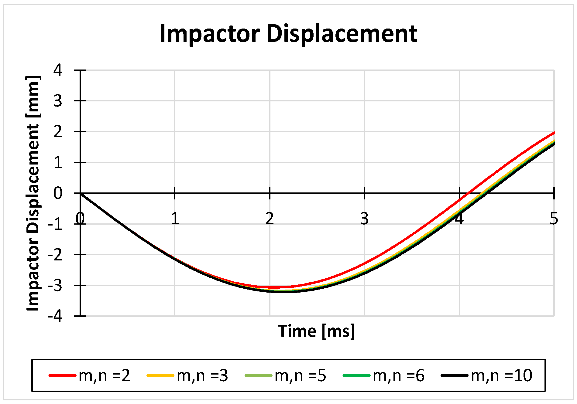
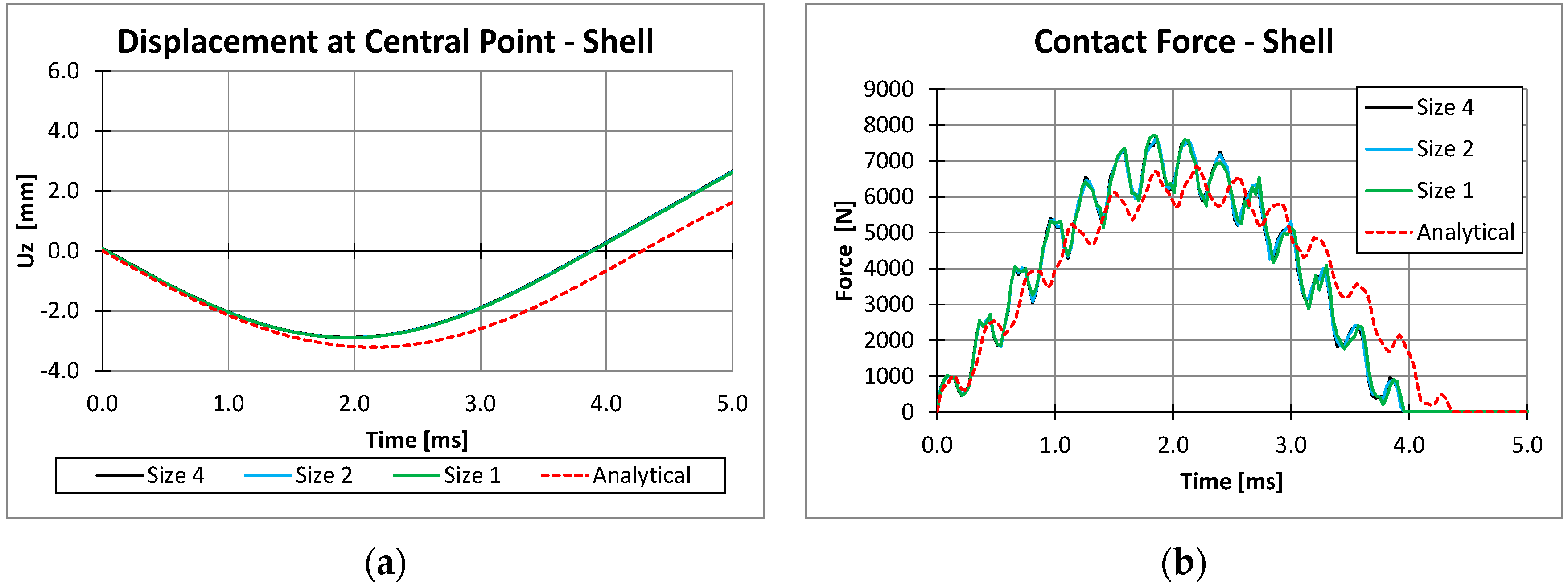
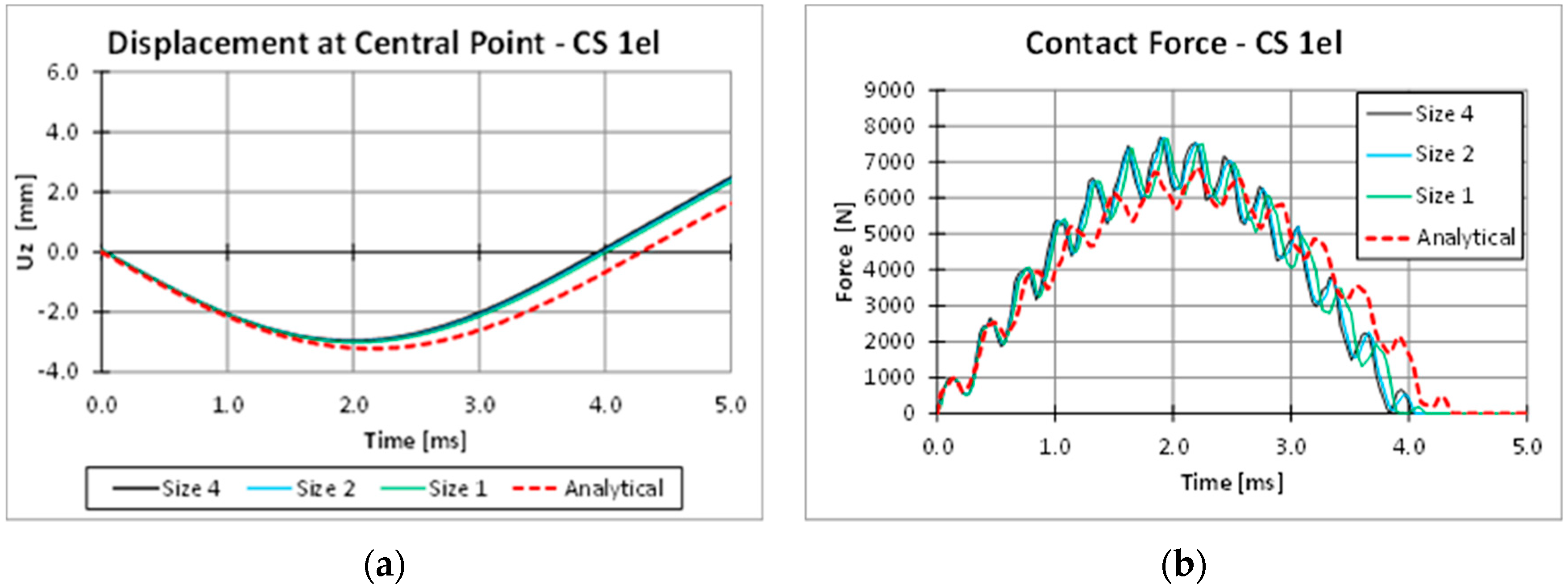
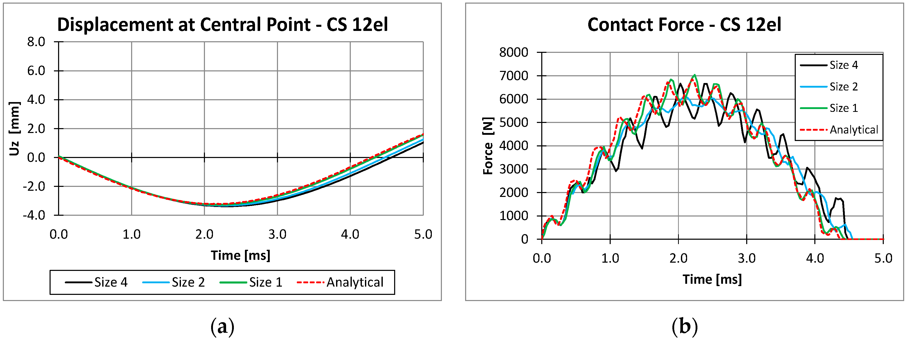
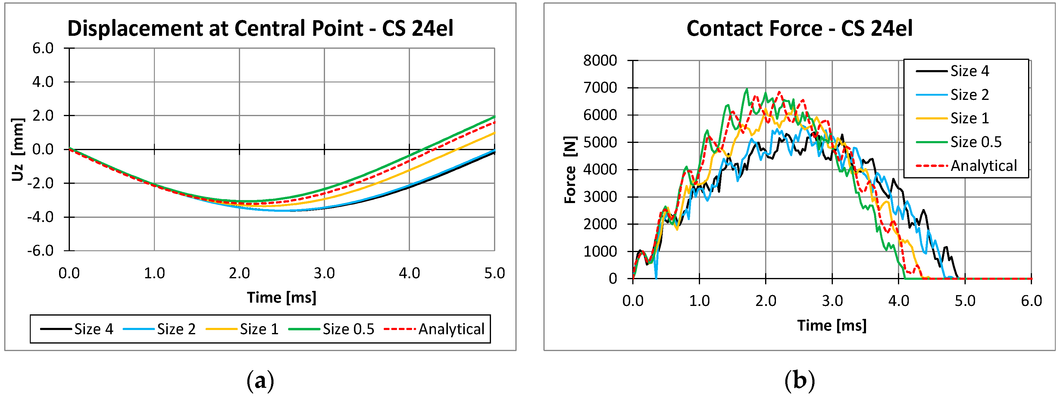
4.1. Preliminary Analyses

The analytical approach results expressed in terms of impactor displacement, contact force, impactor velocity, and kinetic energy versus time are shown respectively in Figure 4, Figure 5, Figure 6 and Figure 7. The results were obtained by considering an increasing number of modes.

Figure 4 and Figure 5 highlight that lower values of m and n results in higher values of stiffness. Indeed, increasing the m and n values led to a decrease of the peak force and to an increase in the maximum deflection of the plate central point. Additionally, according to Figure 4 and Figure 5, the panel response in terms of impact force and maximum deflection tended to converge as the values of m and n increased. Figure 6 shows the trends of the impact velocity considering different m and n values. Although the velocity had the same initial and final values, different m and n led to different velocity trends. Moreover, as a direct consequence of the variation of the impact velocity, the kinetic energy, shown in Figure 7, showed different behavior when low values of m and n were considered. However, as m and n increase, the graphs shown in Figure 4, Figure 5, Figure 6 and Figure 7 appear to be perfectly overlapped.

Then, the numerical results were compared with the analytical ones. The m,n = 10 analytical results were chosen as the reference analytical solution.

In order to define the numerical model which best-fit the analytical results, several parameters were investigated, such as the element type (reduced integration continuum shell elements SC8R and reduced integration solid elements C3D8R), the in-plane element size (1 mm, 2 mm, and 4 mm), and the number of elements along the thickness direction. In particular, Continuum Shell elements were discretized with 1, 12, and 24 elements in the thickness direction, while Solid elements were discretized with 24 elements in the thickness direction (one element per ply). Hence, more than one orientation is associated to the continuum shell elements belonging to the models characterized by less than 24 elements in the thickness direction.

In the numerical analyses, the plate was considered simply supported on the edges, as reported in Figure 8. In the framework of preliminary analyses, aimed to compare the analytical model with the numerical ones to determine the numerical parameters which best represent the mechanical behavior of the plate subjected to low velocity impact, both the inter-laminar and intra-laminar damages were neglected.

In Figure 9, Figure 10, Figure 11, Figure 12 and Figure 13, the numerical and analytical results, in terms of displacement of the impactor and contact force, are compared. In particular, the results shown in Figure 9 were obtained by using a shell element formulation, while the results in Figure 10, Figure 11 and Figure 12 were obtained by using a continuum shell formulation considering, respectively, 1, 12, and 24 elements in the thickness direction. Finally, in Figure 13, the results obtained by using a solid element formulation, with 24 elements in the thickness direction, are introduced.

According to the Figure 9, Figure 10, Figure 11, Figure 12 and Figure 13, Shell and Solid elements’ models were not particularly influenced by the in-plane element size. On the other hand, Continuum shell elements’ models were more sensitive to the in-plane element size as the number of elements in the thickness direction increased. In particular, the numerical results of the Continuum shell model with 12 and 24 elements in the thickness direction associated to coarser mesh (size 2 mm or 4 mm) differed noticeably from the analytical results. This is mainly due to hourglass problems, which can be relevant for the reduced integration scheme elements. Unfortunately, the reduced integration scheme is mandatory in Abaqus/Explicit when Continuum shell elements were adopted. To alleviate hourglass deformation problems that could arise in the numerical models, the default hourglass controls available in Abaqus/Explicit [36] was adopted.

In general, the results highlight that the best results were obtained by the Solid element model discretized with one element per ply and an in-plane element size equal to 1 mm; however, a good numerical–analytical correlation was obtained also by the Continuum shell mode, discretized by 12 elements in the thickness direction and an in-plane element size equal to 1 mm. Indeed, this last configuration was chosen for the analysis presented hereafter due to its excellent compromise between low computational cost and agreement with the analytical solution.

Despite their simplifications, the analytical models available in the literature well describe the behavior of a CFRP plate subjected to impact loading conditions. Hence, the numerical model was validated by comparisons with the analytical one, and the used modeling approach, neglecting in this preliminary phase the damages, has been assessed. Once the accuracy of the impact numerical model is verified, some considerations should be made about the relevant difference between the boundary conditions implemented in the analytical model and the ones implemented in the experimental test. Actually, simply supported conditions have been considered in the analytical and preliminary numerical models; however, the boundary conditions of the experimental test, suggested by the ASTM standards and reported in Figure 14, are substantially different. These boundary conditions are a consequence of a support fixture whose degrees of freedom are restrained and four rigid clamps, also modeled as rigid bodies, which hold the specimen still during impact and avoid any rebound.

A further numerical model obtained with the implementation of the Experimental boundary condition (BC-E) was introduced to understand the effects of boundary conditions on the numerical results. In Figure 15, the analytical, experimental and numerical results of the shell model obtained by considering both analytical (BC-A) and experimental (BC-E) boundary conditions were compared.

In Figure 15, a comparison between experimental, analytical, and numerical results, in terms of force as a function of the time, is reported. The comparison shows that in the first part of the curve both numerical and analytical models were in agreement with the experimental results. However, after a first phase, the analytical model and the FEM BC-A numerical model greatly differed from the experimental result. On the other hand, the FEM BC-E numerical model was characterized by the same mechanical response in terms of stiffness of the laminate, up to the maximum force peak. Indeed, neglecting the damages in the numerical model resulted in grater force peak, if compared with the experiment. Once the accuracy of the numerical model, in terms of elastic response, was established, the numerical models which provided the best results compared to the analytical solution was considered for the final impact test: final Continuum shell model and Final 3D solid model. Since Abaqus does not provide any intra-laminar damage models for Solid elements, a VUMAT was introduced. On the other side, Abaqus built-in Hashin’s criteria were used for model discretized by means of Continuum shell elements. For both the final continuum shell model and the final solid FEM model, gradual material properties degradation rules have been adopted for intra-laminar damage progression and inter-laminar damage were implemented through cohesive elements layers placed at plies interfaces.

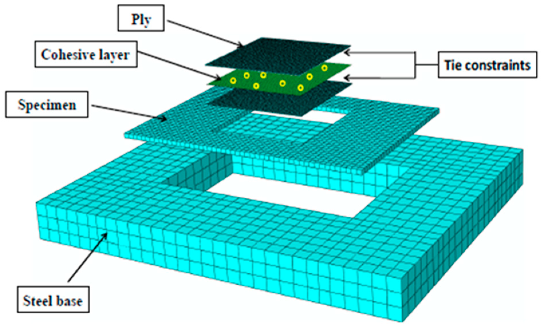
4.2. Final Solid Model

This Final Solid model was created by introducing two different meshed areas connect by a global–local conditions. Indeed, in the specimen impacted area, where most of the damage is supposed to develop (Figure 16) a ply-by-ply refined discretization was considered with each ply represented by a single layer of 3D solid elements C3D8R with a reduced integration scheme. On the contrary, the external global domain has been modeled with a coarser continuum shell mesh. With this discretization scheme, an accurate study can be performed by reducing, at the same time, the computational effort [40].

For 3D solid elements, the intra-laminar damage model introduced in Section 2.2 was applied by means of a VUMAT. Moreover, since the inter-laminar damages are likely to occur only between plies with different fiber orientation, zero-thickness cohesive layers were placed only in these locations. As highlighted in Figure 17, cohesive layers were connected to the adjacent layer by means of tie-constraint.

Table 2. Cohesive mechanical properties.

Property [unit]	Value
En [MPa/mm]	1.155 × 106
Et [MPa/mm]	6 × 105
Es [MPa/mm]	6 × 105
Nmax [MPa]	62.3
Tmax [MPa]	92.3
Smax [MPa]	92.3
GIc [kJ/m2]	0.18
GIIc [kJ/m2]	0.5
GIIIc [kJ/m2]	0.5

reports the mechanical properties of the cohesive material system, which were experimentally evaluated by means of three-point bending (E_n, E_t, E_s), double cantilever beam (N_max, G_Ic), and end notched flexure tests (T_max and S_max, G_IIc and G_IIIc).

Both solid and cohesive elements have been discretized by 1 × 1 mm² elements. The external global domain, which has been modeled by one layer of Continuum shell SC8R elements along thickness direction, has been discretized with an element in-plane size of 4 mm. The specimen is constrained by a fixture and four clamps, modeled with R3D4 rigid elements. The impactor was modeled as a sphere of 16 mm diameter modeled with 3D Solid C3D8R elements. A surface-to-surface contact was used between the impactor and the specimen. During the analysis, the completely damaged elements were removed from the model to increase the computational efficiency. In particular, when cohesive elements were removed, plies can touch each other at the interfaces. Hence, a general contact on the whole model was defined (except for the already defined impact surfaces) to take into account this behavior. A friction coefficient with a value of 0.5 was introduced for both impactor-to-ply contact and ply-to-ply contact. Enhanced hourglass control was set to decrease hourglass problems related to the reduced integrated elements.

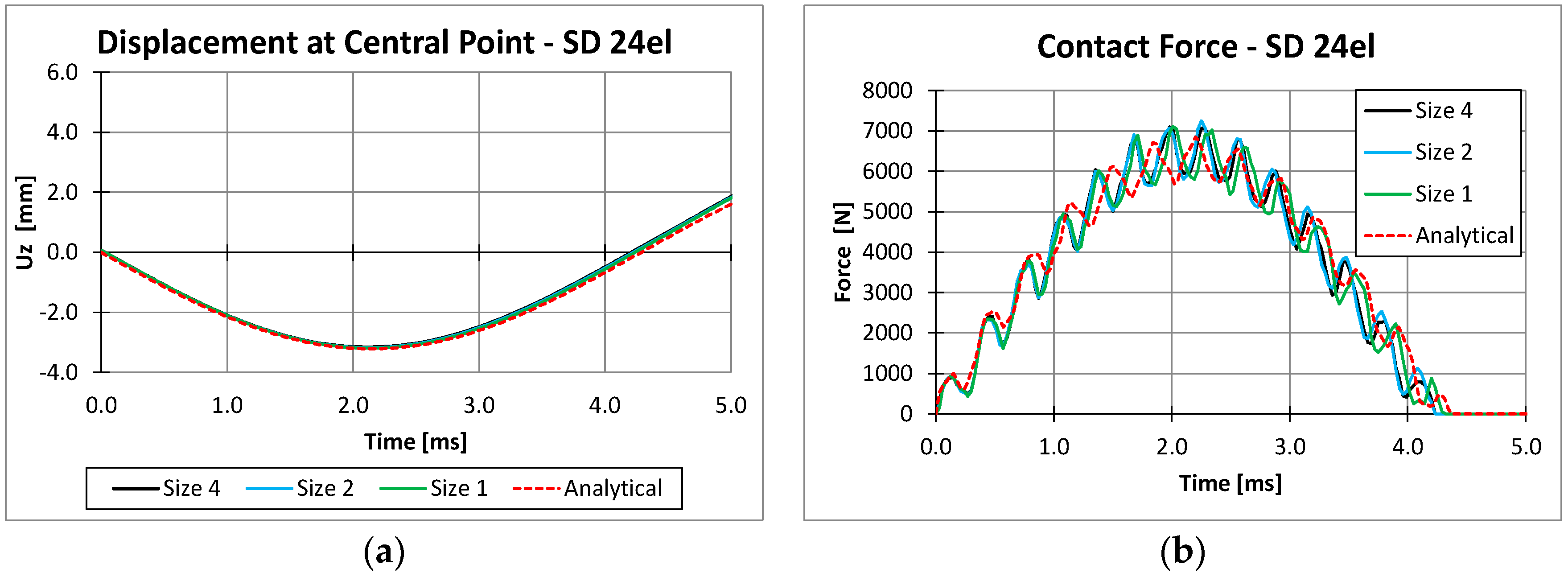
4.3. Final Continuum Shell Model

In the Final Continuum shell model, 12 continuum shell elements along thickness direction were used to model the specimen (Figure 18). For each element, a composite layup composed of two plies was defined.

The intra-laminar damages have been accounted by means of Hashin’s failure criteria, while cohesive layers placed at plies interfaces and introduced in Table 2 were used to model inter-laminar damage. The contact laws introduced in Section 4.2 were adopted.

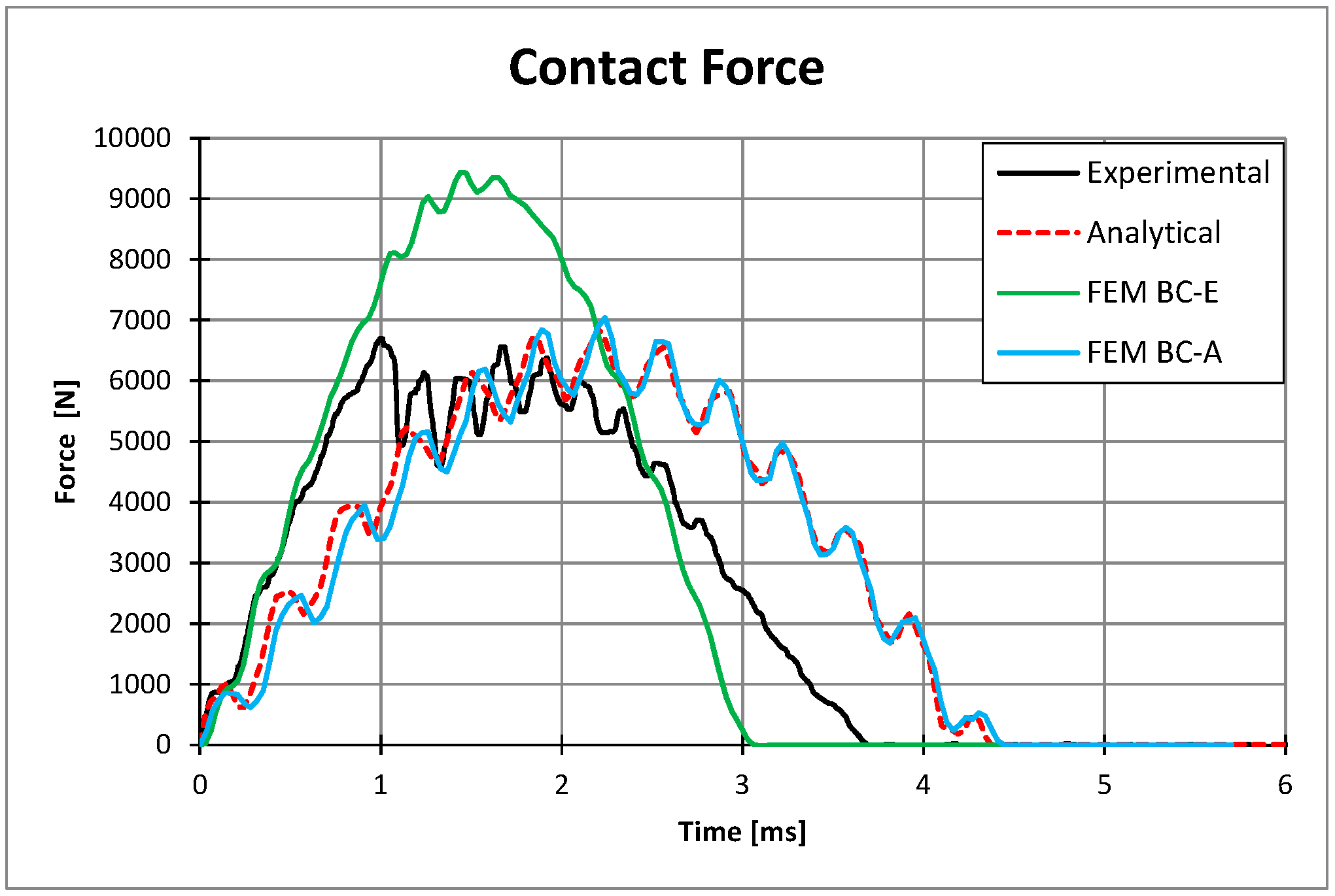
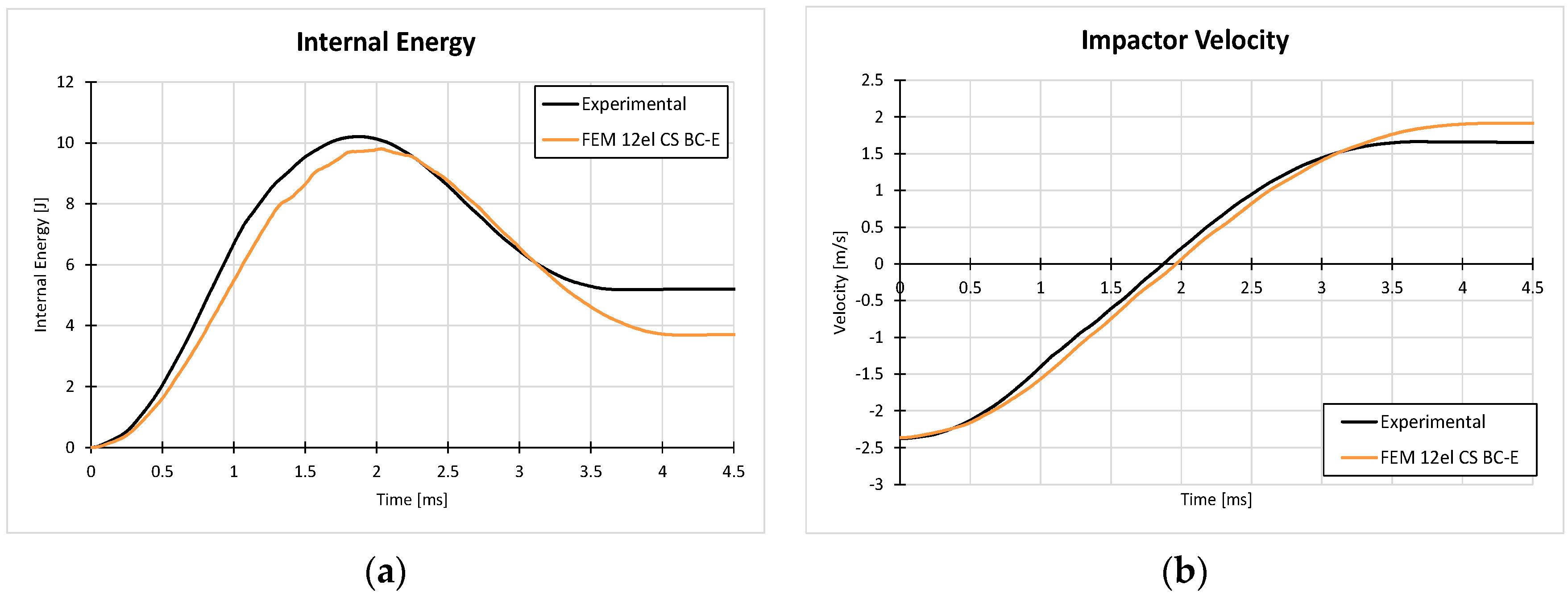
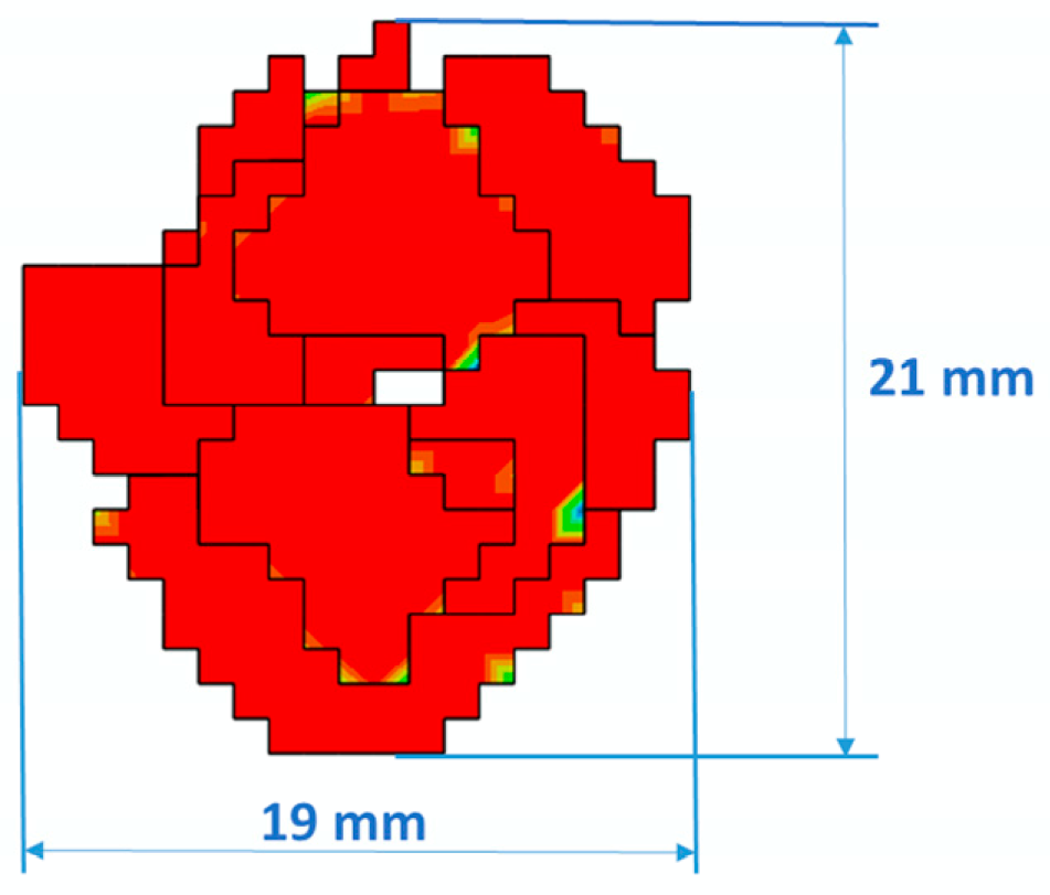
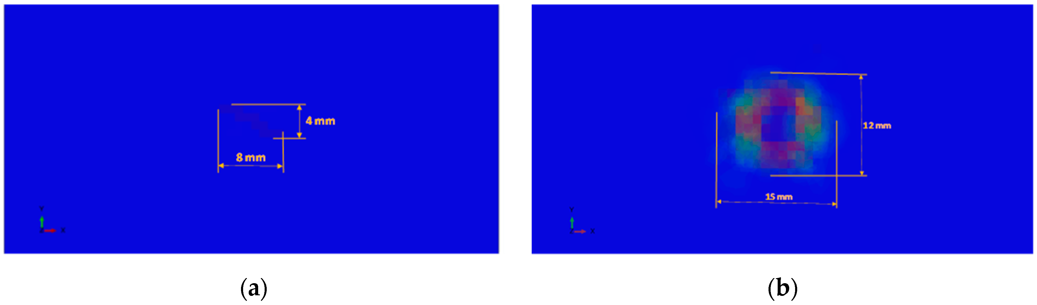
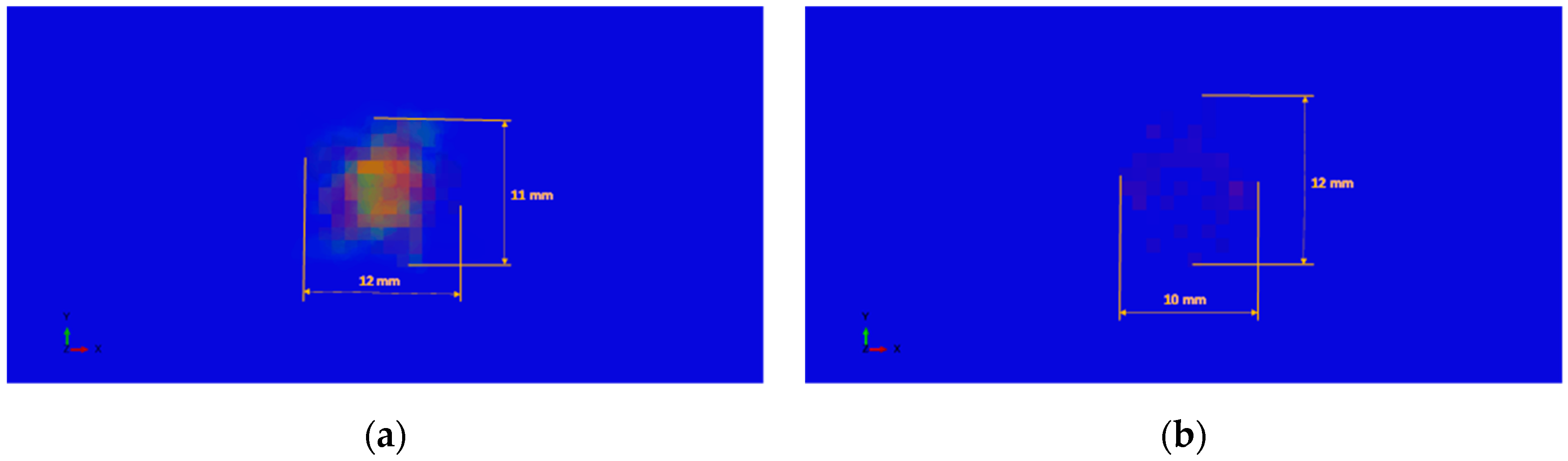
4.4. Numerical–Experimental Correlation

In this section, a comparison between the experimental results and the numerical ones for the both investigated configurations (continuum shell element and solid elements) is performed considering both intra-laminar and inter-laminar damages. Three 10 J impact experimental tests were performed. The damaged area was acquired by means of the ultrasonic C-Scan. Figure 19 shows the C-scan of one representative specimen.

A linear pattern obtained by means of Abaqus/Viewer was used to evaluate the experimental damaged area. The tested specimens were comparable in terms of force, displacement, and kinetic energy as a function of the time, and inter-laminar damages. In particular, the experimental damaged area was about 250 mm², while the numerical damaged area, evaluated by using different numerical models, was in the range 166–609 mm².

The continuum shell model uses a lower number of interfaces between the plies, if compared with the solid element discretization model, and two plies with different orientations are discretized with only one element through the thickness. This assumption could influence the plate mechanical response, leading to different results in terms of delaminated area.

In Figure 20 and Figure 21, the numerical results of the final Continuum shell model in terms of inter-laminar and intra-laminar damages are respectively reported.

According to Figure 20, the simulation over predicts the size of the delamination. This over-prediction can be related to the shell formulation, which is not able to correctly predict the forces acting in the out-of-plane direction, and to the discretization in the thickness direction. Indeed, assuming 12 elements in the thickness direction reduces the number of interfaces where the delamination can occur, leading to larger inter-laminar damages in the remaining interfaces.

Figure 22 and Figure 23 show the predicted and measured contact force, impactor displacement, internal energy, and impactor velocity as a function of the time.

According to Figure 22a, the numerical curve deviates from the experimental one at about 0.3 ms due to anticipated numerical prediction of the onset of delaminations, resulting in a longer contact duration. This effect can be due to the lower number of interfaces. Moreover, the numerically overestimated impactor displacement (6.77% as reported in Figure 22b) and the underestimated residual internal energy of the numerical model (−28.52% as reported in Figure 23a), confirm the over-prediction of damages observed in the simulation. Hence, in the adopted numerical model, significant differences can be observed between the numerical and experimental inter-laminar and intra-laminar damages, as shown in Figure 20 and Figure 21. In particular, the stiffness of the continuum shell element is underestimated if compared with experimental results. Indeed, the maximum displacement of the numerical result is lower than the experimental result in conjunction with a lower peak force.

The numerical results of the solid element model in terms of inter-laminar and intra-laminar damages are reported in Figure 24, Figure 25, Figure 26 and Figure 27.

Figure 24 shows a good agreement between the predicted numerical delaminated area (267 mm²) and the experimental one. Moreover, the delaminations through the specimen sections are reported in Figure 27b. A good agreement between numerical and experimental results has been reached in terms of displacement-time, energy-time, and impact velocity-time as highlighted in Figure 28a,b and Figure 29b. The numerical model with solid element approach is able to predict with good approximation the maximum peak force, with a deviation of −8.90% with respect to the experiment, although it is not able to accurately predict the entire load history. Moreover, the proposed numerical model better predicts the maximum displacement (deviation of 0.37%) and reproduces the overall stiffness of the whole plate. According with Figure 29a, a good correlation in terms of internal energy vs time has been reported. In particular, the solid model compared to the shell one reproduces, in a good way, the amount of energy dissipated in the form of friction, viscosity, and especially due to breakages, is better computed by the solid model (−15.41%) respect to the shell one (−28.52%).

5. Conclusions

In this work, the influence of modeling parameters on the accuracy of results in simulating the impact response of a composites plate subjected to low velocity impact was investigated. Indeed, a numerical procedure has been introduced, able to assess the relevance of modeling parameters for the simulation of intra-laminar and inter-laminar damage onset and progression. In the first stage, an analytical procedure for the prediction of the impact event has been introduced. The results have been used to calibrate the numerical models in terms of element types, element size, and element discretization along the thickness. Continuum shell and solid elements formulations have been analyzed. After this first screening based on analytical–numerical comparisons, continuum shell element model (12 elements through the thickness) and a solid element model (24 elements through the thickness, therefore one element for ply) were selected as the most suitable combination to represent the impact behavior of the specimen. The built-in Abaqus intra-laminar damage model has been used for Continuum Shell elements, while a user defined material model has been developed to simulate the intra-laminar damages in Solid elements, by means of Hashin’s failure criteria and gradual material properties degradation rules. Cohesive zone model elements were adopted to simulate the inter-laminar damage for both the FEM models. The results obtained highlight some important aspects. The firstly introduced analytical method provides a very fast approach in terms of computational costs to preliminary assess the impact behavior of the composite plate. In the secondly introduced numerical model, which neglects the damages and uses a plain strain formulation, the best ratio between accuracy of the results and computational costs is represented by a reduced number of elements in the thickness direction. Then, Abaqus built-in failure criteria for intra-laminar and inter-laminar damage onset and propagation have been used to preliminary assess the damage behavior of the impacted panel. Finally, the solid element formulation, considering both intra-laminar and inter-laminar damages, has been introduced. In particular, user-defined intra-laminar failure criteria (Hashin’s for fiber and tensile matrix, Puck–Shurmann for compressive matrix, and a non-linear behavior of the matrix shear) have been considered, allowing a more accurate prediction of the impact response of the plate. All the presented models provide an increasing degree of accuracy, starting from the analytical to the numerical solid model, being characterized, however, by increasing computational cost.

The results demonstrate the superior capabilities of the solid element model in conjunction with the user material model to simulate the low velocity impact phenomenon on the composite plate, with respect to the shell element model which substantially anticipate the damage onset and overestimates the damages. In conclusion, the solid elements model gives a more realistic representation of the impact behavior of the panel. Indeed, the shell elements formulation does not allow to accurately evaluate the stresses in the normal direction of the plane (which is the predominant direction of deformation during an impact phenomenon) and neglects the effects of the shear.

References

1. Abrate, S. Impact on Composite Structures; Cambridge University Press: Cambridge, UK, 1998. [Google Scholar]
2. Abrate, S. Impact Engineering of Composites Structures; Springer: Wien, Austria; Udine, Italy, 2011. [Google Scholar]
3. Zhang, X. Low Velocity Impact and Damage Tolerance of Composite Aircraft Structures; Cranfield University: Cranfield, UK, 2003. [Google Scholar]
4. Soutis, C.; Curtis, P. Prediction of the post-impact compressive strength of CFRP laminated composites. Compos. Sci. Technol. 1996, 56, 677–684. [Google Scholar] [CrossRef]
5. Wisnom, M. The role of delamination in failure of fibre-reinforced composites. Philos. Trans. R. Soc. 2012, 370, 1850–1870. [Google Scholar] [CrossRef] [PubMed]
6. Abrate, S. Modeling of impacts on composite structures. Compos. Struct. 2001, 51, 129–138. [Google Scholar] [CrossRef]
7. Christoforou, A.; Swanson, S. Analysis of impact response in composite plates. Int. J. Solid Struct. 1991, 27, 161–170. [Google Scholar] [CrossRef]
8. Carvalho, A.; Guedes Soares, C. Dynamic response of rectangular plates of composite materials subjected to impact loads. Compos. Struct. 1996, 34, 55–63. [Google Scholar] [CrossRef]
9. Gonzàlez, E.; Maimì, P.; Camanho, P.; Turon, A.; Mayugo, J. Simulation of drop-weight impact and compression after impact tests on composite laminates. Compos. Struct. 2012, 94, 3364–3378. [Google Scholar] [CrossRef]
10. Barile, C.; Casavola, C.; Pappalettera, G.; Vimalathithan, P.K. Acousto-ultrasonic evaluation of interlaminar strength on CFRP laminates. Compos. Struct. 2019, 208, 796–805. [Google Scholar] [CrossRef]
11. Olsson, R. Analytical prediction of large mass impact damage in composite laminates. Compos.-Part A Appl. Sci. Manuf. 2001, 32, 1207–1215. [Google Scholar] [CrossRef]
12. Olsson, R. Closed form prediction of peak load and delamination onset under small mass impact. Compos. Struct. 2003, 59, 341–349. [Google Scholar] [CrossRef]
13. Olsson, R. Analytical prediction of damage due to large mass impact on thin ply composites. Compos.-Part A Appl. Sci. Manuf. 2015, 72, 184–191. [Google Scholar] [CrossRef]
14. Huang, K.Y.; De Boer, A.; Akkerman, R. Analytical modeling of impact resistance and damage tolerance of laminated composite plates. AIAA J. 2008, 46, 2760–2772. [Google Scholar] [CrossRef]
15. Tita, V.; deCarvalho, J.; Vandepitte, D. Failure analysis of low velocity impact on thin composite laminates: Experimental and numerical approaches. Compos. Struct. 2008, 83, 413–428. [Google Scholar] [CrossRef]
16. Li, C.; Hu, N.; Yin, Y.; Sekine, H.; Fukunaga, H. Low-velocity impact-induced damage of continuous fiber-reinforced composite laminates. Part I: An FEM numerical model. Composites 2002, 33, 1055–1062. [Google Scholar] [CrossRef]
17. Elder, D.; Thomson, R.; Nguyen, M.; Scott, M. Review of delamination predictive methods for low speed impact of composite laminates. Compos. Struct. 2004, 66, 677–683. [Google Scholar] [CrossRef]
18. Riccio, A.; Caputo, F.; Di Felice, G.; Saputo, S.; Toscano, C.; Lopresto, V. A Joint Numerical-Experimental Study on Impact Induced Intra-laminar and Inter-laminar Damage in Laminated Composites. Appl. Compos. Mater. 2016, 23, 219–237. [Google Scholar] [CrossRef]
19. Riccio, A.; Raimondo, A.; Saputo, S.; Sellitto, A.; Battaglia, M.; Petrone, G. A numerical study on the impact behavior of natural fibres made honeycomb cores. Compos. Struct. 2018, 202, 909–916. [Google Scholar] [CrossRef]
20. Li, N.; Chen, P.H. Micro–macro FE modeling of damage evolution in laminated composite plates subjected to low velocity impact. Compos. Struct. 2016, 147, 111–121. [Google Scholar] [CrossRef]
21. Faggiani, A.; Falzon, B.G. Predicting low-velocity impact damage on a stiffened composite panel. Compos.-Part A Appl. Sci. Manuf. 2010, 41, 737–749. [Google Scholar] [CrossRef]
22. Falzon, B.G.; Apruzzese, P. Numerical analysis of intralaminar failure mechanisms in composite structures. Part I: FE implementation. Compos. Struct. 2011, 93, 1039–1046. [Google Scholar] [CrossRef]
23. Falzon, B.G.; Apruzzese, P. Numerical analysis of intralaminar failure mechanisms in composite structures. Part II: Applications. Compos. Struct. 2011, 93, 1047–1053. [Google Scholar] [CrossRef]
24. Tay, T. Characterization and analysis of delamination fracture in composites: An overview of developments from 1990 to 2001. Appl. Mech. Rev. 2003, 56, 1–32. [Google Scholar] [CrossRef]
25. Wisnom, M. Modeling discrete failures in composites with interface elements. Compos. Part A 2010, 41, 795–805. [Google Scholar] [CrossRef]
26. Camanho, P.; Davila, C. Mixed-Mode Decohesion Finite Elements for the Simulation of Delamination in Composite Materials; NASA/TM-2002-211737; National Aeronautics and Space Administration, Langley Research Center: Hampton, VA, USA, 2002; pp. 1–37. [Google Scholar]
27. Riccio, A.; Russo, A.; Sellitto, A.; Raimondo, A. Development and application of a numerical procedure for the simulation of the “Fibre Bridging” phenomenon in composite structures. Compos. Struct. 2017, 168, 104–119. [Google Scholar] [CrossRef]
28. Riccio, A.; Ricchiuto, R.; Di Caprio, F.; Sellitto, A.; Raimondo, A. Numerical investigation of constitutive material models on bonded joints in scarf repaired composite laminates. Eng. Fract. Mech. 2017, 173, 91–106. [Google Scholar] [CrossRef]
29. Aymerich, F.; Dore, F.; Priolo, P. Simulation of multiple delaminations in impacted cross-ply laminates using a finite element model based on cohesive interface elements. Compos. Sci. Technol. 2009, 69, 1699–1709. [Google Scholar] [CrossRef]
30. DeMoura, M.; Gonçalves, J. Modeling the interaction between matrix cracking and delamination in carbon–epoxy laminates under low velocity impact. Compos. Sci. Technol. 2004, 64, 1021–1027. [Google Scholar] [CrossRef]
31. Zhang, Y.; Zhu, P.; Lai, X. Finite element analysis of low-velocity impact damage in composite laminated plates. Mater. Des. 2006, 27, 513–519. [Google Scholar] [CrossRef]
32. deBorst, R.; Remmers, J.J.; Needleman, A. Mesh-independent discrete numerical representations of cohesive-zone models. Eng. Fract. Mech. 2006, 73, 160–177. [Google Scholar]
33. Maimì, P.; Camanho, P.; Mayugo, J.; Davila, C. A continuum damage model for composite laminates: Part I—Constitutive model. Mech. Mater. 2007, 39, 897–908. [Google Scholar] [CrossRef]
34. ASTM D7136/D-Standard Test Method for Measuring the Damage Resistance of a Fiber-Reinforced Polymer Matrix Composite to a Drop-Weight Impact Event; ASTM International: West Conshohocken, PA, USA, 2005.
35. Sellitto, A.; Borrelli, R.; Caputo, F.; Riccio, A.; Scaramuzzino, F. Application to plate components of a kinematic global-local approach for non-matching finite element meshes. Int. J. Struct. Integr. 2012, 3, 260–273. [Google Scholar] [CrossRef]
36. Dassault System Abaqus 2016 User’s Manual; Dassault Systèmes Simulia Corp.: Providence, RI, USA, 2016.
37. Christoforou, A.; Yigit, A. Effect of flexibility on low velocity impact response. J. Sound Vib. 1998, 217, 563–578. [Google Scholar] [CrossRef]
38. Puck, A.; Schurmann, H. Failure analysis of FRP laminates by means of physically based phenomenological models. Compos. Sci. Technol. 1998, 58, 1045–1067. [Google Scholar] [CrossRef]
39. Bazant, Z.P.; Oh, B.H. Crack band theory for fracture of concrete. Mater. Struct. 1983, 16, 155–177. [Google Scholar] [Green Version]
40. Davies, G.A.O.; Olsson, R. Impact on composite structures. Aeronaut. J. 2004, 108, 541–563. [Google Scholar] [CrossRef]
Figure 1. Compressive matrix failure and fracture plane.
Applsci 09 02372 g001
Figure 2. Constitutive relation adopted for fiber and matrix failure modes in tension and compression.
Applsci 09 02372 g002
Figure 3. Experimental set-up.
Applsci 09 02372 g003
Figure 4. Analytical solution—impactor displacement.
Applsci 09 02372 g004
Figure 5. Analytical solution—contact force history.
Applsci 09 02372 g005
Figure 6. Analytical solution—impactor velocity.
Applsci 09 02372 g006
Figure 7. Analytical solution—kinetic energy.
Applsci 09 02372 g007
Figure 8. Shell model boundary conditions.
Applsci 09 02372 g008
Figure 9. Shell elements: analytical–numerical comparison. (a) Central point displacement; (b) contact force.
Applsci 09 02372 g009
Figure 10. Continuum shell elements with one element in the thickness direction: analytical–numerical comparison. (a) Central point displacement; (b) contact force.
Applsci 09 02372 g010
Figure 11. Continuum shell elements with 12 elements in the thickness direction: analytical–numerical comparison. (a) Central point displacement; (b) contact force.
Applsci 09 02372 g011
Figure 12. Continuum shell elements with 24 elements in the thickness direction: analytical–numerical comparison. (a) Central point displacement; (b) contact force.
Applsci 09 02372 g012
Figure 13. Solid elements with 24 elements in the thickness direction: analytical–numerical comparison. (a) Central point displacement; (b) contact force.
Applsci 09 02372 g013
Figure 14. Boundary conditions. (a) Analytical; (b) experimental.
Applsci 09 02372 g014
Figure 15. Contact force comparison between analytical and numerical boundary conditions.
Applsci 09 02372 g015
Figure 16. Domain and boundary conditions.
Applsci 09 02372 g016
Figure 17. Exploded model (detail).
Applsci 09 02372 g017
Figure 18. Continuum shell elements domain.
Applsci 09 02372 g018
Figure 19. C-scan of the damaged area.
Applsci 09 02372 g019
Figure 20. Shell element model: delamination.
Applsci 09 02372 g020
Figure 21. Shell element model: intra-laminar damages (envelope).
Applsci 09 02372 g021
Figure 22. Shell element model. (a) Contact force history; (b) impactor displacement.
Applsci 09 02372 g022
Figure 23. Shell element model. (a) Internal energy; (b) impactor velocity.
Applsci 09 02372 g023
Figure 24. Solid element model: delamination.
Applsci 09 02372 g024
Figure 25. (a) Fiber compressive damage; (b) matrix tensile damage.
Applsci 09 02372 g025
Figure 26. (a) Matrix compressive damage; (b) longitudinal shear damage.
Applsci 09 02372 g026
Figure 27. (a) Transversal Shear damage; (b) specimen section detail.
Applsci 09 02372 g027
Figure 28. (a) Contact force history; (b) impactor displacement.
Applsci 09 02372 g028
Figure 29. (a) Internal energy; (b) impactor velocity.
Applsci 09 02372 g029