Sentiment Classification Using Convolutional Neural Networks


Abstract
:1. Introduction
2. Background
2.1. Machine Learning for Sentiment Classification
2.2. Deep Learning for Sentiment Classification
2.3. Convolutional Neural Network for Text Classification
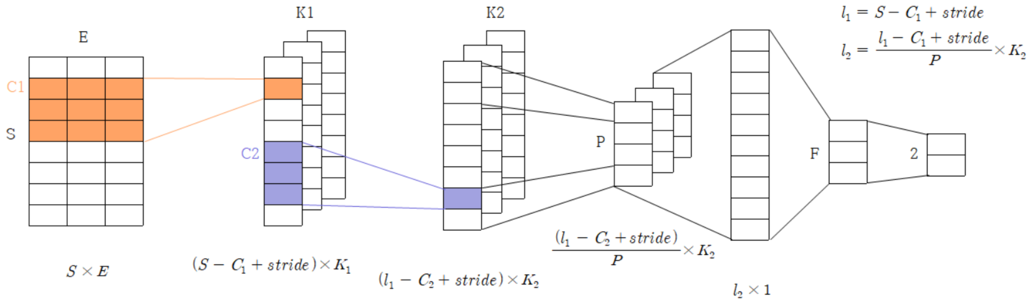
3. The Proposed Method
4. Experiment
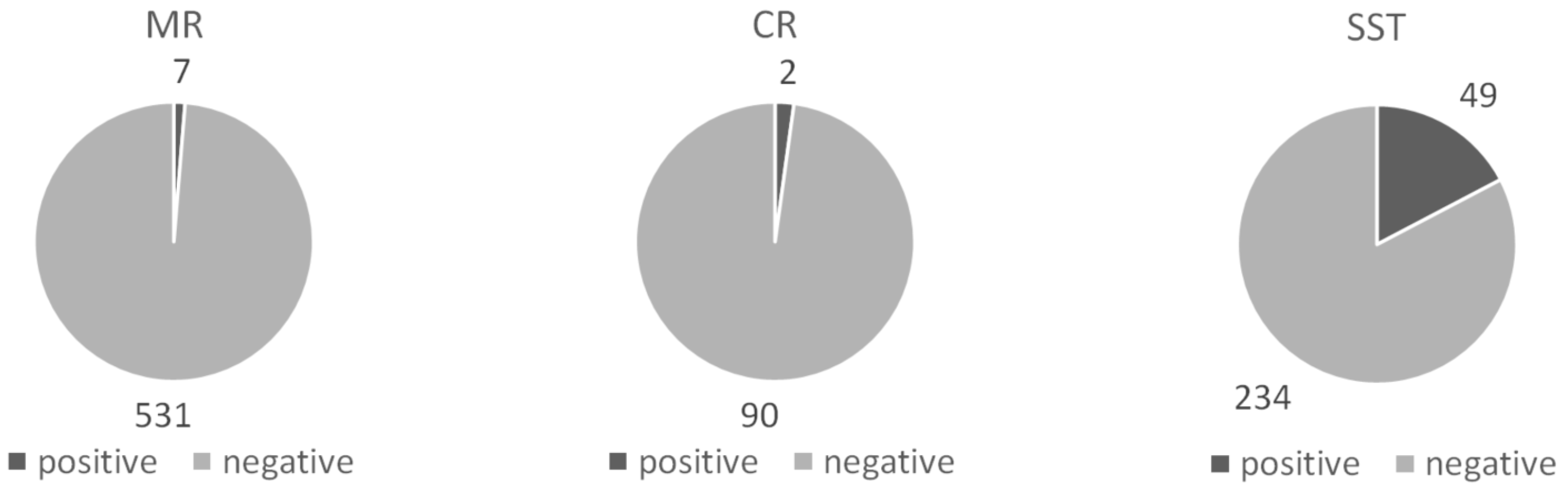
4.1. Data
4.2. Preprocessing
4.3. Performance Comparison
5. Result and Discussion
5.1. Result
5.2. Discussion
5.2.1. Comparison with Other Models
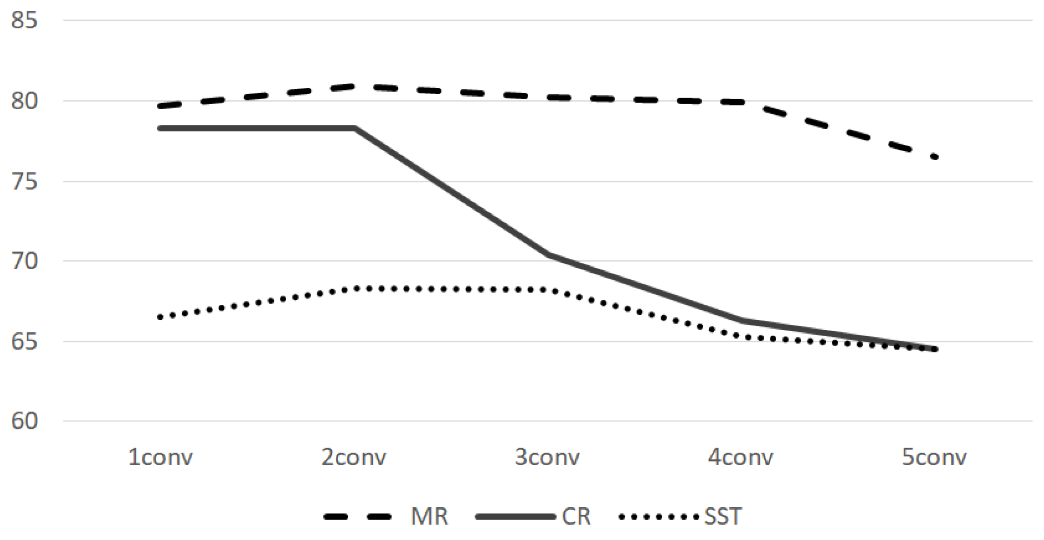
5.2.2. Network Structure
6. Conclusions
Author Contributions
Acknowledgments
Conflicts of Interest
References
- Kim, Y. Convolutional neural networks for sentence classification. arXiv 2014, arXiv:1408.5882. [Google Scholar]
- Nal, K.; Grefenstette, E.; Blunsom, P. A convolutional neural network for modelling sentences. arXiv 2014, arXiv:1404.2188. [Google Scholar]
- Lei, T.; Barzilay, R.; Jaakkola, T. Molding cnns for text: Non-linear, non-consecutive convolutions. arXiv 2015, arXiv:1508.04112. [Google Scholar]
- Amazon Movie Review Dataset. Available online: https://www.kaggle.com/ranjan6806/corpus2#corpus/ (accessed on 11 November 2012).
- Movie Review Dataset. Available online: https://www.kaggle.com/ayanmaity/movie-review#train.tsv/ (accessed on 11 November 2012).
- Rotten Tomatoes Movie Review Dataset. Available online: https://www.kaggle.com/c/movie-review-sentiment-analysis-kernels-only/ (accessed on 11 November 2012).
- Consumer Reviews Of Amazon Products Dataset. Available online: https://www.kaggle.com/datafiniti/consumer-reviews-of-amazon-products/ (accessed on 11 November 2012).
- Stanford Sentiment Treebank Dataset. Available online: https://nlp.stanford.edu/sentiment/code.html/ (accessed on 11 November 2012).
- Pak, A.; Paroubek, P. Twitter as a corpus for sentiment analysis and opinion mining. LREc 2010, 10, 1320–1326. [Google Scholar]
- Alm, C.O.; Roth, D.; Sproat, R. Emotions from text: Machine learning for text-based emotion prediction. In Proceedings of the Conference on Human Language Technology and Empirical Methods in Natural Language Processing, Vancouver, BC, Canada, 6–8 October 2005; pp. 579–586. [Google Scholar]
- Bartlett, M.S.; Littlewort, G.; Frank, M.; Lainscsek, C.; Fasel, I.; Movellan, J. Recognizing facial expression: Machine learning and application to spontaneous behavior. In Proceedings of the 2005 IEEE Computer Society Conference on Computer Vision and Pattern Recognition (CVPR’05), San Diego, CA, USA, 20–25 June 2005; Volume 2, pp. 568–573. [Google Scholar]
- Heraz, A.; Razaki, R.; Frasson, C. Using machine learning to predict learner emotional state from brainwaves. In Proceedings of the Seventh IEEE International Conference on Advanced Learning Technologies (ICALT 2007), Niigata, Japan, 18–20 July 2007; pp. 853–857. [Google Scholar]
- Yujiao, L.; Fleyeh, H. Twitter Sentiment Analysis of New IKEA Stores Using Machine Learning. In Proceedings of the International Conference on Computer and Applications, Beirut, Lebanon, 25–26 July 2018. [Google Scholar]
- Read, J. Using emoticons to reduce dependency in machine learning techniques for sentiment classification. In Proceedings of the ACL Student Research Workshop, Ann Arbor, Michigan, 27 June 2005; pp. 43–48. [Google Scholar]
- Kennedy, A.; Inkpen, D. Sentiment classification of movie reviews using contextual valence shifters. Comput. Intell. 2006, 22, 110–125. [Google Scholar] [CrossRef]
- Jiang, L.; Yu, M.; Zhou, M.; Liu, X.; Zhao, T. Target-dependent twitter sentiment classification. In Proceedings of the 49th Annual Meeting of the Association for Computational Linguistics: Human Language Technologies, Portland, Oregon, 19–24 June 2011; Volume 1, pp. 151–160. [Google Scholar]
- Neethu, M.; Rajasree, R. Sentiment analysis in twitter using machine learning techniques. In Proceedings of the 2013 Fourth International Conference on Computing, Communications and Networking Technologies (ICCCNT), Tiruchengode, India, 4–6 July 2013; pp. 1–5. [Google Scholar]
- Gautam, G.; Yadav, D. Sentiment analysis of twitter data using machine learning approaches and semantic analysis. In Proceedings of the 2014 Seventh International Conference on Contemporary Computing (IC3), Noida, India, 7–9 August 2014; pp. 437–442. [Google Scholar]
- Tripathy, A.; Agrawal, A.; Rath, S.K. Classification of sentiment reviews using n-gram machine learning approach. Expert Syst. Appl. 2016, 57, 117–126. [Google Scholar] [CrossRef]
- Wan, X. A comparative study of cross-lingual sentiment classification. In Proceedings of the 2012 IEEE/WIC/ACM International Joint Conferences on Web Intelligence and Intelligent Agent Technology, Macau, China, 4–7 December 2012; Volume 1, pp. 24–31. [Google Scholar]
- Akaichi, J. Social networks’ Facebook’statutes updates mining for sentiment classification. In Proceedings of the 2013 International Conference on Social Computing, Alexandria, VA, USA, 8–14 September 2013; pp. 886–891. [Google Scholar]
- Denecke, K. Using sentiwordnet for multilingual sentiment analysis. In Proceedings of the 2008 IEEE 24th International Conference on Data Engineering Workshop, Cancun, Mexico, 7–12 April 2008; pp. 507–512. [Google Scholar]
- Bahrainian, S.A.; Dengel, A. Sentiment analysis using sentiment features. In Proceedings of the 2013 IEEE/WIC/ACM International Joint Conferences on Web Intelligence (WI) and Intelligent Agent Technologies (IAT), Atlanta, GA, USA, 17–20 November 2013; Volume 3, pp. 26–29. [Google Scholar]
- Antai, R. Sentiment classification using summaries: A comparative investigation of lexical and statistical approaches. In Proceedings of the 2014 6th Computer Science and Electronic Engineering Conference (CEEC), Colchester, UK, 25–26 September 2014; pp. 154–159. [Google Scholar]
- Hasan, A.; Moin, S.; Karim, A.; Shamshirband, S. Machine learning-based sentiment analysis for twitter accounts. Math. Comput. Appl. 2018, 23, 11. [Google Scholar] [CrossRef]
- Mensikova, A.; Mattmann, C.A. Ensemble sentiment analysis to identify human trafficking in web data. In Proceedings of the Workshop on Graph Techniques for Adversarial Activity Analytics (GTA 2018), Marina Del Rey, CA, USA, 5–9 February 2018. [Google Scholar]
- Pang, B.; Lee, L. A sentimental education: Sentiment analysis using subjectivity summarization based on minimum cuts. In Proceedings of the 42nd Annual Meeting on Association for Computational Linguistics, Barcelona, Spain, 21–26 July 2004; pp. 271–278. [Google Scholar]
- Valakunde, N.; Patwardhan, M. Multi-aspect and multi-class based document sentiment analysis of educational data catering accreditation process. In Proceedings of the 2013 International Conference on Cloud & Ubiquitous Computing & Emerging Technologies, Pune, India, 15–16 November 2013; pp. 188–192. [Google Scholar]
- Yassine, M.; Hajj, H. A framework for emotion mining from text in online social networks. In Proceedings of the 2010 IEEE International Conference on Data Mining Workshops, Sydney, Australia, 13 December 2010; pp. 1136–1142. [Google Scholar]
- Karamibekr, M.; Ghorbani, A.A. A structure for opinion in social domains. In Proceedings of the 2013 International Conference on Social Computing, Alexandria, VA, USA, 8–14 September 2013; pp. 264–271. [Google Scholar]
- Ghiassi, M.; Lee, S. A domain transferable lexicon set for Twitter sentiment analysis using a supervised machine learning approach. Expert Syst. Appl. 2018, 106, 197–216. [Google Scholar] [CrossRef]
- Balazs, J.A.; Velásquez, J.D. Opinion mining and information fusion: A survey. Inf. Fusion 2016, 27, 95–110. [Google Scholar] [CrossRef]
- Chaturvedi, I.; Cambria, E.; Welsch, R.E.; Herrera, F. Distinguishing between facts and opinions for sentiment analysis: Survey and challenges. Inf. Fusion 2018, 44, 65–77. [Google Scholar] [CrossRef]
- Dong, L.; Wei, F.; Tan, C.; Tang, D.; Zhou, M.; Xu, K. Adaptive recursive neural network for target-dependent twitter sentiment classification. In Proceedings of the 52nd Annual Meeting of the Association for Computational Linguistics (Volume 2: Short Papers), Baltimore, MD, USA, 23–25 June 2014; Volume 2, pp. 49–54. [Google Scholar]
- Huang, M.; Cao, Y.; Dong, C. Modeling rich contexts for sentiment classification with lstm. arXiv 2016, arXiv:1605.01478. [Google Scholar]
- Tang, D.; Qin, B.; Liu, T. Document modeling with gated recurrent neural network for sentiment classification. In Proceedings of the 2015 Conference on Empirical Methods in Natural Language Processing, Lisbon, Portugal, 17–21 September 2015; pp. 1422–1432. [Google Scholar]
- Qian, Q.; Huang, M.; Lei, J.; Zhu, X. Linguistically regularized lstms for sentiment classification. arXiv 2016, arXiv:1611.03949. [Google Scholar]
- Mikolov, T. Statistical language models based on neural networks. Ph.D. Thesis, Brno University of Technology, Brno, Czechia, 2012. [Google Scholar]
- Chung, J.; Gulcehre, C.; Cho, K.; Bengio, Y. Empirical evaluation of gated recurrent neural networks on sequence modeling. arXiv 2014, arXiv:1412.3555. [Google Scholar]
- Tai, K.S.; Socher, R.; Manning, C.D. Improved semantic representations from tree-structured long short-term memory networks. arXiv 2015, arXiv:1503.00075. [Google Scholar]
- Wang, F.; Zhang, Z.; Lan, M. Ecnu at semeval-2016 task 7: An enhanced supervised learning method for lexicon sentiment intensity ranking. In Proceedings of the 10th International Workshop on Semantic Evaluation (SemEval-2016), San Diego, CA, USA, 16–17 June 2016; pp. 491–496. [Google Scholar]
- Zhang, Y.; Zhang, Z.; Miao, D.; Wang, J. Three-way enhanced convolutional neural networks for sentence-level sentiment classification. Inf. Sci. 2019, 477, 55–64. [Google Scholar] [CrossRef]
- Severyn, A.; Moschitti, A. Unitn: Training deep convolutional neural network for twitter sentiment classification. In Proceedings of the 9th International Workshop On Semantic Evaluation (SemEval 2015), Denver, CO, USA, 4–5 June 2015; pp. 464–469. [Google Scholar]
- Deriu, J.; Lucchi, A.; De Luca, V.; Severyn, A.; Müller, S.; Cieliebak, M.; Hofmann, T.; Jaggi, M. Leveraging large amounts of weakly supervised data for multi-language sentiment classification. In Proceedings of the 26th International Conference on World Wide Web, Perth, Australia, 3–7 April 2017; pp. 1045–1052. [Google Scholar]
- Ouyang, X.; Zhou, P.; Li, C.H.; Liu, L. Sentiment analysis using convolutional neural network. In Proceedings of the 2015 IEEE International Conference on Computer and Information Technology; Ubiquitous Computing and Communications; Dependable, Autonomic and Secure Computing; Pervasive Intelligence and Computing, Liverpool, UK, 26–28 October 2015; pp. 2359–2364. [Google Scholar]
- Socher, R.; Huval, B.; Manning, C.D.; Ng, A.Y. Semantic compositionality through recursive matrix-vector spaces. In Proceedings of the 2012 Joint Conference on Empirical Methods in Natural Language Processing and Computational Natural Language Learning, Jeju Island, Korea, 12–14 July 2012; pp. 1201–1211. [Google Scholar]
- Rios, A.; Kavuluru, R. Convolutional neural networks for biomedical text classification: Application in indexing biomedical articles. In Proceedings of the 6th ACM Conference on Bioinformatics, Computational Biology and Health Informatics, Atlanta, GA, USA, 9–12 September 2015; pp. 258–267. [Google Scholar]
- Zhang, X.; Zhao, J.; LeCun, Y. Character-level convolutional networks for text classification. In Advances in Neural Information Processing Systems 28; Neural Information Processing Systems Foundation, Inc.: Montreal, QC, Canada, 2015; pp. 649–657. [Google Scholar]
- Yih, W.T.; He, X.; Meek, C. Semantic Parsing for Single-Relation Question Answering. In Proceedings of the 52nd Annual Meeting of the Association for Computational Linguistics, Baltimore, MD, USA, 23–25 June 2014; Volume 2, pp. 643–648. [Google Scholar]
- Shen, Y.; Xiaodong, H.; Gao, J.; Deng, L.; Mensnil, G. Learning Semantic Representations Using Convolutional Neural Networks for Web Search. In Proceedings of the 23rd International Conference on World Wide Web, Seoul, Korea, 7–11 April 2014; pp. 373–374. [Google Scholar]
- Lai, S.; Xu, L.; Liu, K.; Zhao, J. Recurrent convolutional neural networks for text classification. In Proceedings of the Twenty-Ninth AAAI Conference on Artificial Intelligence, Austin, TX, USA, 25–30 January 2015. [Google Scholar]
- Gehring, J.; Auli, M.; Grangier, D.; Dauphin, Y.N. A convolutional encoder model for neural machine translation. arXiv 2016, arXiv:1611.02344. [Google Scholar]
- Dos Santos, C.; Gatti, M. Deep convolutional neural networks for sentiment analysis of short texts. In Proceedings of the COLING 2014, the 25th International Conference on Computational Linguistics: Technical Papers, Dublin, Ireland, 23–29 August 2014; pp. 69–78. [Google Scholar]
- Boser, B.E.; Guyon, I.M.; Vapnik, V.N. A training algorithm for optimal margin classifiers. In Proceedings of the Fifth Annual Workshop on Computational Learning Theory, Pittsburgh, PA, USA, 27–29 July 1992; pp. 144–152. [Google Scholar]
- Breiman, L. Random forests. Mach. Learn. 2001, 45, 5–32. [Google Scholar] [CrossRef]
- Szegedy, C.; Liu, W.; Jia, Y.; Sermanet, P.; Reed, S.; Anguelov, D.; Erhan, D.; Vanhoucke, V.; Rabinovich, A. Going deeper with convolutions. In Proceedings of the 2015 IEEE Conference on Computer Vision and Pattern Recognition, Boston, MA, USA, 7–12 June 2015; pp. 1–9. [Google Scholar]
- Szegedy, C.; Vanhoucke, V.; Ioffe, S.; Shlens, J.; Wojna, Z. Rethinking the inception architecture for computer vision. In Proceedings of the IEEE Conference on Computer Vision and Pattern Recognition, Las Vegas, NV, USA, 27–30 June 2016; pp. 2818–2826. [Google Scholar]
- Szegedy, C.; Ioffe, S.; Vanhoucke, V.; Alemi, A.A. Inception-v4, inception-resnet and the impact of residual connections on learning. In Proceedings of the Thirty-First AAAI Conference on Artificial Intelligence, San Francisco, CA, USA, 4–9 February 2017. [Google Scholar]


| Data | N | Dist (+,−) | aveL/maxL | Train:Test:Val | ∣V∣ |
|---|---|---|---|---|---|
| MR | 21,498 | 55:45 | 31/290 | 12,095:5375:4031 | 9396 |
| CR | 3671 | 62:38 | 19/227 | 2064:918:689 | 1417 |
| SST | 11,286 | 52:48 | 12/41 | 6348:2822:2116 | 3550 |
| Model | Description |
|---|---|
| Naive Bayes (NB) |
|
| Decision Tree (DT) |
|
| Support Vector Machine (SVM) |
|
| Random Forest (RF) |
|
| Model | Accuracy | Precision | Recall | F1 | Weighted-F1 |
|---|---|---|---|---|---|
| Decision Tree | 59.64 | 58.0/64.0 | 76.2/39.6 | 67.4/47.1 | 57.2 |
| Naive Bayes | 56.40 | 57.5/53.3 | 77.7/30.7 | 66.1/38.9 | 52.0 |
| Support Vector Machine | 54.95 | 57.7/55.2 | 93.0/9.1 | 69.3/15.5 | 44.9 |
| Random Forest | 58.73 | 56.4/59.8 | 74.7/39.4 | 66.4/46.4 | 58.1 |
| Kim [1] | 80.85 | 80.7/80.9 | 76.2/84.7 | 78.3/82.8 | 80.75 |
| Zhang et al. [42] | 77.28 | 72.4/69.1 | 56.1/82.1 | 63.2/75.0 | 69.62 |
| Emb+Conv+Conv+Pool+FC | 81.06 | 81.5/80.7 | 75.6/85.6 | 78.4/83.1 | 80.96 |
| Emb+Conv+Pool+FC | 79.70 | 77.4/81.63 | 78.2/80.9 | 77.8/81.3 | 79.71 |
| Emb+Conv+Conv+Conv+Pool+FC | 80.30 | 80.2/80.4 | 75.3/84.5 | 77.7/82.4 | 80.26 |
| Emb+Conv+Pool+Conv+FC | 78.17 | 74.4/81.8 | 79.5/77.1 | 76.8/79.4 | 78.22 |
| Emb+Conv+globalpool+FC | 77.54 | 77.3/77.7 | 71.8/82.4 | 74.4/79.9 | 77.39 |
| Emb+Conv+Conv+globalpool+FC | 79.06 | 79.1/79.0 | 73.5/83.8 | 76.2/81.3 | 78.98 |
| Emb+Conv+Pool+Conv+Pool+FC | 79.11 | 78.6/79.5 | 74.3/83.1 | 76.4/81.2 | 79.0 |
| Emb+Conv+Pool+Conv+Pool+Conv+Pool+FC | 74.61 | 84.1/72.8 | 59.5/90.6 | 69.7/80.7 | 75.7 |
| Model | CR | SST | ||
|---|---|---|---|---|
| Weighted-F1 | F1 | Weighted-F1 | F1 | |
| Decision Tree | 63.7 | 47.0/74.5 | 51.5 | 62.4/41.7 |
| Naive Bayes | 61.0 | 77.7/31.8 | 35.7 | 10.6/63.4 |
| Support Vector Machine | 59.7 | 26.5/78.5 | 37.8 | 68.6/4.0 |
| Random Forest | 64.4 | 41.8/76.9 | 51.2 | 59.0/47.3 |
| Kim [1] | 74.8 | 78.6/65.6 | 56.1 | 47.2/66.3 |
| Zhang et al. [42] | 54.8 | 64.7/37.7 | 52.1 | 45.6/59.5 |
| Emb+Conv+Conv+Pool+FC | 78.3 | 84.8/67.1 | 68.3 | 70.5/65.7 |
| Emb+Conv+Pool+FC | 78.3 | 82.3/71.3 | 66.5 | 67.7/65.1 |
| Emb+Conv+Conv+Conv+Pool+FC | 70.4 | 82.0/50.3 | 68.2 | 68.4/68.0 |
| Emb+Conv+Pool+Conv+FC | 75.3 | 84.0/60.3 | 68.6 | 70.5/66.5 |
| Emb+Conv+globalpool+FC | 81.4 | 86.1/73.4 | 70.2 | 72.8/67.2 |
| Emb+Conv+Conv+globalpool+FC | 79.4 | 84.5/70.5 | 70.0 | 71.2/68.7 |
| Emb+Conv+Pool+Conv+Pool+FC | 73.18 | 82.8/56.5 | 66.62 | 67.7/65.4 |
| Emb+Conv+Pool+Conv+Pool+Conv+Pool+FC | 51.57 | 77.6/6.7 | 65.21 | 70.2/59.5 |
| Model | Weighted-F1 |
|---|---|
| Decision Tree | 46.8 |
| Naive Bayes | 27.2 |
| Support Vector Machine | 34.9 |
| Random Forest | 46.2 |
| Kim [1] | 68.2 |
| Zhang et al. [42] | 67.5 |
| Emb+Conv+Conv+Pool+FC | 68.3 |
| Emb+Conv+Pool+FC | 55.0 |
| Emb+Conv+Conv+Conv+Pool+FC | 64.6 |
| Emb+Conv+Pool+Conv+FC | 66.9 |
| Emb+Conv+globalpool+FC | 65.3 |
| Emb+Conv+Conv+globalpool+FC | 67.5 |
© 2019 by the authors. Licensee MDPI, Basel, Switzerland. This article is an open access article distributed under the terms and conditions of the Creative Commons Attribution (CC BY) license (http://creativecommons.org/licenses/by/4.0/).
Share and Cite
Kim, H.; Jeong, Y.-S. Sentiment Classification Using Convolutional Neural Networks. Appl. Sci. 2019, 9, 2347. https://doi.org/10.3390/app9112347
Kim H, Jeong Y-S. Sentiment Classification Using Convolutional Neural Networks. Applied Sciences. 2019; 9(11):2347. https://doi.org/10.3390/app9112347
Chicago/Turabian StyleKim, Hannah, and Young-Seob Jeong. 2019. "Sentiment Classification Using Convolutional Neural Networks" Applied Sciences 9, no. 11: 2347. https://doi.org/10.3390/app9112347
APA StyleKim, H., & Jeong, Y.-S. (2019). Sentiment Classification Using Convolutional Neural Networks. Applied Sciences, 9(11), 2347. https://doi.org/10.3390/app9112347