Article

Visual Saliency Detection Using a Rule-Based Aggregation Approach

by
Alberto Lopez-Alanis
1,
Rocio A. Lizarraga-Morales
2,*,
Raul E. Sanchez-Yanez
1,
Diana E. Martinez-Rodriguez
1 and
Marco A. Contreras-Cruz
1
1
Departamento de Ingeniería Electrónica, DICIS, Universidad de Guanajuato, Salamanca 36885, Mexico
2
Departamento Arte y Empresa, DICIS, Universidad de Guanajuato, Salamanca 36885, Mexico
*
Author to whom correspondence should be addressed.
Appl. Sci. 2019, 9(10), 2015; https://doi.org/10.3390/app9102015
Submission received: 13 April 2019 / Revised: 9 May 2019 / Accepted: 9 May 2019 / Published: 16 May 2019
(This article belongs to the Section Electrical, Electronics and Communications Engineering)

Abstract

:
In this paper, we propose an approach for salient pixel detection using a rule-based system. In our proposal, rules are automatically learned by combining four saliency models. The learned rules are utilized for the detection of pixels of the salient object in a visual scene. The proposed methodology consists of two main stages. Firstly, in the training stage, the knowledge extracted from outputs of four state-of-the-art saliency models is used to induce an ensemble of rough-set-based rules. Secondly, the induced rules are utilized by our system to determine, in a binary manner, the pixels corresponding to the salient object within a scene. Being independent of any threshold value, such a method eliminates any midway uncertainty and exempts us from performing a post-processing step as is required in most approaches to saliency detection. The experimental results on three datasets show that our method obtains stable and better results than state-of-the-art models. Moreover, it can be used as a pre-processing stage in computer vision-based applications in diverse areas such as robotics, image segmentation, marketing, and image compression.

1. Introduction

It is well-known that humans cannot observe every detail on an entire scene at first glance. The human visual system focuses its attention on certain regions of a given scene according to their saliency. Koch et al. [1] defined saliency as the extent to which an object stands out from its surrounding regions. Visual saliency detection systems aim at identifying the salient regions from a given image, and it is a fundamental task that has been addressed in recent years. The saliency detection has been used as an important pre-processing stage in a number of computer vision applications such as image compression [2,3,4], object recognition [5,6,7], marketing or signaling [8,9,10], and robot navigation [11,12,13], among others.
Among the proposals for visual saliency detection, we identify two main approaches: fixation prediction and salient object detection. The first one is used to determine only the human gaze locations. The second one is used to extract the most relevant objects within the scene. According to Borji et al. [14], fixation prediction models are limited because they only provide points and some of them can be isolated from others. On the other hand, the salient object detection provides a whole region within the image, which can be used for a higher level process. Predicting accurately the region that humans will observe is a relevant aspect that any saliency detection approach must accomplish.
Based on the saliency detection approaches that can be found in the existing literature, we may classify the algorithms into individual or aggregation models. The first category corresponds to models that make use of intrinsic information from the image to perform a saliency prediction task, i.e., using mainly low-level features such as color or contrast, without any prior knowledge about the image. Generally, individual models use biological theories, purely computational formulations, or a combination of both [15]. The first individual model is the seminal work presented by Itti et al. [16]. In his research work, Itti estimated the saliency of a given pixel incorporating the cognitive theory presented by Treisman and Gelade [17], which suggests that the human visual system responds to contrast stimulus in color, orientation, and intensity. In addition, this model takes into account the computational architecture proposed by Koch and Ullman [1]. From this work onwards, many approaches have been proposed based on the same cognitive assumptions. As examples of this type of approach, we can mention the proposals by Frintrop et al. [18,19], Parkhurst et al. [20], and Lemur et al. [21]. Additionally, other individual models came up to the scene taking into account not only pixel-level information but also regional and global cues. As an example of these types of models, we can mention the approach proposed by Achacnta et al. [15] where the saliency is estimated as the difference between the pixel color and the color average of the image. In the research work of Cheng et al. [22], two approaches are introduced. The first approach computes saliency as the distance in color between pixels. The second approach considers saliency as the weighted color distance between regions. Perazzi et al. [23] proposed a method for saliency detection based on feature contrast, where uniqueness and spatial distribution of regions into the image are computed using a high dimensional Gaussian filter. Based on the concept that salient regions are distinctive to their local and global surrounding, Goferman et al. [24] proposed their context-aware saliency detection model. Recently, Huang et al. [25] proposed a model which considers global contrast in different directions for each pixel in the CIELAB color space.
The main goal of a saliency detection model is to estimate saliency in a scene, determining if a location of a given image is salient or not. Usually, the saliency information is encoded in a saliency map (SM) which is a two-dimensional representation given in grayscale [26]. In the SM, the clearest location corresponds to the most salient region and the darkest location to the less salient region. If we think of the saliency map as a binary classifier [27], where we represent whether a location of an image is salient or not, then the individual models offer only partial results. The outcomes from individual models need post-processing such as thresholding or segmentation to obtain a binary saliency map.
To combine to the best characteristics of individual models, the second category of models is proposed: aggregation and learning models. Aggregation models or learning techniques, attempt to combine in different manners the outcomes of individual saliency detection models in order to obtain a more robust result.
Several direct combination techniques have been proposed to overcome the deficiencies of individual approaches, such as in the research work of Borji et al. [14]. In that work, Borji presented four combination techniques for saliency aggregation from a probabilistic point of view. Such techniques are Naive Bayesian evidence accumulation and linear summation of identity, exponential, and logarithm functions. Note that the goal of these techniques is to exploit the outcomes of different individual methods to generate a new saliency map, which gives a more accurate saliency estimation. In the research work of Mai et al. [28], a data-driven combination approach based on the conditional random field (CRF) framework is presented. Based on this framework, Mai considered the interaction between neighboring pixels and modeled the contribution of each individual saliency map. In addition, Mai presented in the same research work the Pixel-Wise aggregation model (PW). In this approach, the aggregation is performed by weighting diverse results of individual saliency detection models. The weights are learned by using a standard logistic regression. Although these approaches are found to be effective in distinct cases, they present failures when detecting ambiguous cases, since the combination criterion is not flexible. Additionally, the output of these methods still needs a binarization stage.
Recently, deep learning has been used to address saliency detection tasks. In the proposal of Wang et al. [29], a deep neural network is used to estimate saliency locally. Then, the obtained saliency map is refined by exploiting high-level object concepts. Zhao et al. [30] employed global and local context in a unified multi-context convolutional neural network. Liu and Han [31] proposed a two-stage saliency detection frame based on convolutional neural networks. The architecture proposed estimates saliency by learning from global saliency cues. Then, a refinement process is carried out incorporating local context information. To obtain more accurate boundaries and compact saliency maps, Hu et al. [32] proposed a deep network incorporating a level set function. Besides, a superpixel-based guided filter is incorporated as a layer of the network, allowing to obtain a full resolution saliency map. Chen et al. [33] applied attention weight in a top-down manner to filter out a noisy response from the background. In addition, a saliency refinement network is proposed to improve the resolution of the saliency map by using a second-order term to introduce nonlinearity in the learning process. Despite the remarkable performance of the learning approaches mentioned above, the outcome obtained is still given as a gray-level saliency map. Furthermore, the neural network performs as black-box which makes difficult the human-comprehension of the obtained saliency model [34].
In this paper, we propose an aggregation system for salient object detection using individual descriptors in a rule-based approach. According to Napierala and Stefanowski [34], rules are one of the most popular representations of knowledge. The rules are more human-comprehensible than other representations of knowledge [35], which is useful when constructing intelligent systems. Specifically, we explore the use of rough-set-based rules for the saliency determination of a given pixel within an image. The rough set theory is a mathematical approach introduced by Pawlak [36], useful for dealing with vagueness and uncertainty in data analysis. The rough sets are useful when it is not possible to represent a concept with a precise criterion [37]. According to Tay and Shen [38], rough sets discover patterns hidden in data. Additionally, the set of obtained rules gives an overall description of the data, eliminating redundancy present in the original data. Exploiting the main advantage of rough set theory, which is that it does not need any additional information about the data [39], we propose a combination of four different state-of-the-art methods as feature descriptors included in the rules: Saliency Filter (SF) [23], Minimum Barrier Salient Object Detection (MBS) [40], Region-based Contrast (RC) [22], and Minimum Directional Contrast (MDC) [25]. The selection criteria of these methods correspond to how saliency is computed. MDC and MBS estimate saliency in a pixel-wise manner, whereas SF and RC compute saliency in a region-based manner. The four models chosen as feature descriptors perform saliency detection in CIELAB color space, which is a perceptual color space [22]. These features extract different kinds of salient information from the image. Our method automatically decodes the knowledge found by each individual model and combines the four features in a useful way. The output obtained from our proposal is given in a binary manner, where each pixel position is evaluated as salient or not, eliminating any midway uncertainty. Therefore, our proposal exempts us from implementing any post-processing required to obtain a binary saliency map. The proposed method was evaluated on three extensive and challenging databases designed for saliency detection. Experiments showed that our method leads to better results in comparison to other state-of-the-art methods. From now on, we call our method RSD, for Rough-set-based Saliency Detection.
The remainder of this paper is organized as follows: In Section 2, the proposed approach is described, along with the methods used to estimate the features. In Section 3, we describe the experiments performed on three databases to validate our method. Finally, Section 4 presents a summary of this work and our concluding remarks.

2. Methodology

In this section we introduce the proposed RSD and its theoretical background. An overview of the proposed approach is illustrated in Figure 1. Firstly, in Figure 1a, the rule-based learning process is depicted. At the beginning, feature extraction is performed by computing saliency maps of four state-of-the-art approaches. After that, the four saliency maps are submitted to the rough-set-based system. The main goal of such system is to obtain knowledge from saliency maps to build rules from their combination. The resulting saliency prediction rules indicate if a given pixel is salient or not, without the need of any post-processing. The process to test the model for saliency detection at pixel-level on an incoming image is depicted in Figure 1b. Each block of Figure 1 is detailed in the next subsections.

2.1. Rough-Set-Based Rules

The rough set theory was introduced by Pawlak [36] as a mathematical tool for dealing with imperfect and inconsistent data, in order to extract useful knowledge. In a classification process, an object is described in terms of a set of attributes. The information contained on these sets of attributes usually has a certain level of vagueness and ambiguity. Rough set approaches handle inconsistencies of data using two types of approximation sets, the lower and the upper approximations. If we consider I as the information system used to approximate to decision class X. The lower approximation I ̲ X , determines according to I, the objects that certainly correspond to class X. The upper approximation, I ¯ X , defines the objects that possibly correspond to class X. In Equations (1) and (2), we present the definition of the lower and upper approximations, respectively, where [ x ] I is the elementary set containing x X .
I ̲ X = { x | [ x ] I X } ,
I ¯ X = { x | [ x ] I X } .
The difference between the lower and upper approximations is known as the region boundary and is defined as in Equation (3). If the region boundary is not empty, the set is a rough set.
I N I ( X ) = I ¯ X - I ̲ X .
From the given information, the rough set algorithm produces an ensemble of rules. Usually, the rules obtained are represented in the logical form of I F ( a n t e c e d e n t ) T H E N ( c o n s e q u e n t ) . For our purposes, the left side of the rule, called a n t e c e d e n t , is an attribute condition or feature. The right side of the rule is the c o n s e q u e n t , i.e., the decision class or saliency.
The rules created by using the rough set algorithm can be categorized into three types of rules sets [41]. The smallest set of rules needed to describe an object is known as the minimum set of rules. In contrast, the exhaustive set of rules consist of all the rules that can be generated from the examples given for learning. Finally, the satisfactory set of rules is conformed by those rules that satisfy requirements previously defined by the user. Therefore, several methods have been proposed to rough-set-based rule generation. One of the most commonly used rough-set-based approaches is the method proposed by Stefanowski, named MODLEM [42].The main advantage of this method relies on the capability of handling discretization of the information and rule induction simultaneously. Additionally, the MODLEM algorithm generates a minimal set of rules for every decision class [35]. In the MODLEM algorithm, for numerical attributes, an elementary condition t is defined in the form of either ( a < v ) or ( a > = v ) , where v is a threshold on the attribute domain and a is a numerical attribute value [43]. To determine the elementary condition, the values of a numerical attribute a are sorted in increasing order to find cut-points. The cut-points correspond to the mid-points between the sorted values. A cut-point is evaluated using either the class entropy technique or Laplace accuracy, and the elementary condition is selected by the largest coverage on the given learning examples. This procedure is repeated until the complete rule is induced and the set of rules obtained is minimum. In our experiments, we utilized the MODLEM implementation at WEKA [44], an open-source data mining tool.

2.2. Feature Extraction

Antecedents in rule-based approaches are features that describe a given object or class. The proposed RSD system uses grayscale saliency maps as input features. We utilize four state-of-the-art saliency detection models: Minimum Barrier Salient Object Detection (MBS) [40], Minimum Directional Contrast (MDC) [25], Region-based Contrast (RC) [22], and Saliency Filter (SF) [23]. As far as we know, these methods are the state-of-the-art of individual models for saliency detection. In addition, the selected methods are recent and achieve a good performance in the saliency detection task. The experimentation that led us to select these four saliency models for aggregation purposes is detailed in Section Below, we present a brief description of these saliency models.
Minimum Barrier Salient Object Detection. The saliency detection model proposed by Zhang et al. [40] aims to highlight a salient object within a scene. By using the minimum barrier distance, the Minimum Barrier Salient Object Detection (MBS) model exploits the boundary connectivity hint. Visiting each x pixel position on the image, each adjacent y pixel is taken into account to minimize the path cost at x. The minimization function is defined in Equation (4).
D ( x ) m i n D ( x ) , β I ( P ( y ) · x , y ) ,
where D ( x ) is the distance that is desired to calculate, P ( y ) represents the actual path assigned to pixel position y and y , x is the existing edge from y to x. Being P ( y ) · y , x denoted by P y ( x ) , the cost function proposed in this work is represented as in Equation (5).
β I ( P y ( x ) ) = max { U ( y ) , I ( x ) } - min { L ( y ) , I ( x ) } ,
where U ( y ) is the highest pixel value on P ( y ) and L ( y ) is the lowest pixel value on P ( y ) .
The saliency map obtained from this model is given as a gray-level image, where the intensity of each pixel represents the estimated saliency level. Hence, if a binary output is needed, thresholding shall be performed.
Minimum Directional Contrast. To detect salient objects in images, Huang and Zhang [25] proposed the Minimum Directional Contrast (MDC) saliency detection model. The MDC model takes into account the spatial distribution of contrast. The main contribution of this model is a metric to estimate saliency, which is called Minimum Directional Contrast (MDC). Saliency is estimated in a pixel-wise manner and using an input image in the CIELAB color space. The input image is divided into four regions, taking the inspected pixel x as the center of the image. Each region is a box delimited by four points: top left (TL), top right (TR), bottom left (BL), and bottom right (BR). Then, the directional contrast for each region is defined as in Equation (6).
D C i , Ω = j Ω c h = 1 K ( I i , c h - I j , c h ) 2 .
In this research work, the authors introduced an interesting property about the distribution of contrast between regions and the examined pixel. If the pixel i belongs to the foreground of the image, the contrast in all directions is high. On the contrary, if the pixel belongs to the background of the image, the contrast is low in one direction. The raw saliency measure is estimated as the minimum contrast of the four regions, which is defined in Equation (7).
S ( i ) = min Ω T L , T R , B L , B R D C i , Ω = min Ω T L , T R , B L , B R j Ω c h = 1 K ( I i , c h - I j , c h ) 2 .
Because the saliency map is given in grayscale, the authors proposed a saliency enhancement using a post-processing step.
Region-based Contrast. Cheng et al. [22] proposed the Region Based Contrast (RC) model to salient object detection. The RC method considers the contrast between regions to estimate saliency. Firstly, the incoming image in CIELAB color space is segmented into regions. A color histogram of the obtained regions is computed and is used to estimate color contrast between regions. Hence, the saliency is computed as in Equation (8).
S ( r k ) = r k r i ω ( r i ) D r ( r k , r i ) ,
where ω ( r i ) is the weight assigned to the region r i and D r ( · , · ) is the color distance metric between two regions.
The outcome of the RC model is a grayscale saliency map. Hence, the authors proposed a segmentation algorithm named SaliencyCut, which is based on an enhancement of the GrabCut [45] segmentation approach.
Saliency Filter. The Saliency Filter (SF) method was proposed by Perazzi et al. [23] for salient object detection. This model considers rarity and spatial distribution to compute saliency. Given an input image in CIELAB color space, a segmentation of the incoming image is performed by using geodesic image distance. The uniqueness metric is calculated by Equation (9).
U i = j = 1 N c i - c j 2 ω ( p i , p j ) w i j ( p ) ,
where c i is the inspected segment of the image, c j is the rest of the segments of the image, and w i j ( p ) is a Gaussian weight position function to control the influence rarity of the inspected region.
The spatial distribution of an element is estimated by the spatial variance of its color, according to Equation (10),
D i = j = 1 N p j - μ i 2 ω ( c i , c j ) w i j ( c ) ,
where w i j ( c ) represents a similarity measure of color c i and c j of the segments i and j, p j is the location of the inspected segment and μ i is the Gaussian weighted mean position of color c i . Later, both metrics obtained are combined for each segment of the image by using Equation (11).
S i = U i · e x p ( - k · D i ) ,
where k is a normalization factor for the exponential function. Finally, the saliency estimation of each pixel is computed as in Equation (12).
S ˜ i = j = 1 N ω i j S j ,
where S j is the surrounding of the pixel and w i j is a Gaussian weight. In the same manner as the aforementioned models, the final saliency map from SF model is given as a grayscale image. A post-processing is required to obtain a binary map with the salient regions segmented.

2.3. Learning a Saliency Model

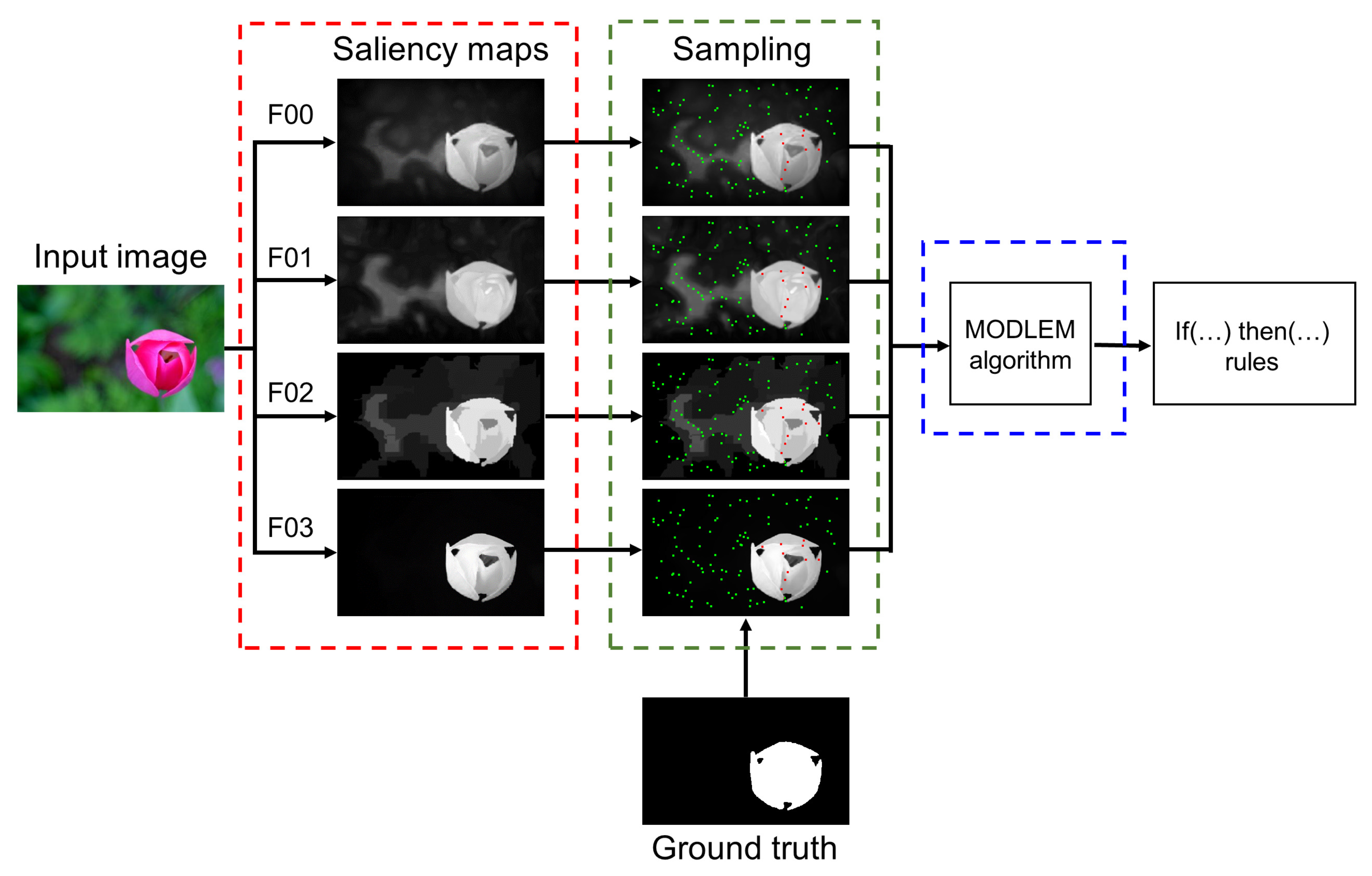
Our goal is to take advantage of the outcomes from individual saliency detection methods to construct a saliency prediction model by using a rough-set-based learning algorithm. In Figure 2 we present the illustration of the learning process.
Basically, the learning process has been divided into three main stages. As the initial stage of our proposed method, we perform a feature extraction process on a given dataset. To clearly define the feature extraction process, let us consider four output images from state-of-the-art individual models: F 00 ( x , y ) , F 01 ( x , y ) , F 02 ( x , y ) , and F 03 ( x , y ) . They are all SMs with K different gray levels and ( M × N ) pixel size. For each pixel P located in the coordinates ( x , y ) , ( x , y ) D , D = { 0 , , M - 1 } × { 0 , , N - 1 } , we obtain its corresponding gray value from each saliency map in such a way that each pixel can be represented by four values or features: P ( x , y ) = { F 00 , F 01 , F 02 , F 03 } . Secondly, we label each P ( x , y ) taking into account the ground truth. Since the ground truth is provided as a binary map, we can classify pixels as non-salient or salient using values of 0 and 1, respectively.
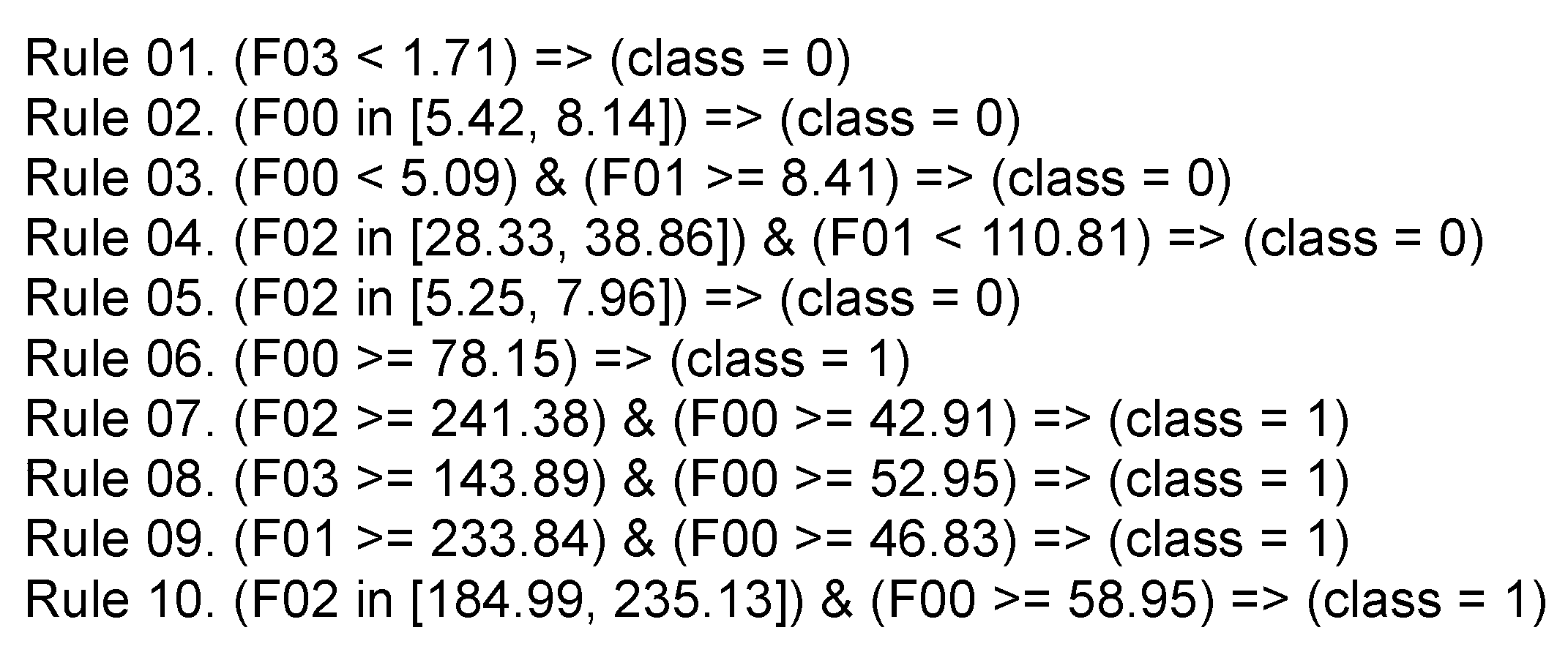
Thirdly, to make the training faster, we randomly sample the saliency maps. One hundred samples per image gave us the best result. We chose 90% of the samples corresponding to the non-salient class. Conversely, the 10% of the samples belong to the salient class. The set of samples are taken and submitted to the learning process by using the MODLEM algorithm. In Figure 3, we show an example of a set of the rules obtained; this set of rules is used in a later stage to saliency prediction.

3. Experimental Results

In this section, we present and compare the results obtained by our proposed system RSD and state-of-the-art methods. In addition, we give a description of the datasets used, parameter settings, and performance metrics.

3.1. Datasets and Quantitative Metrics

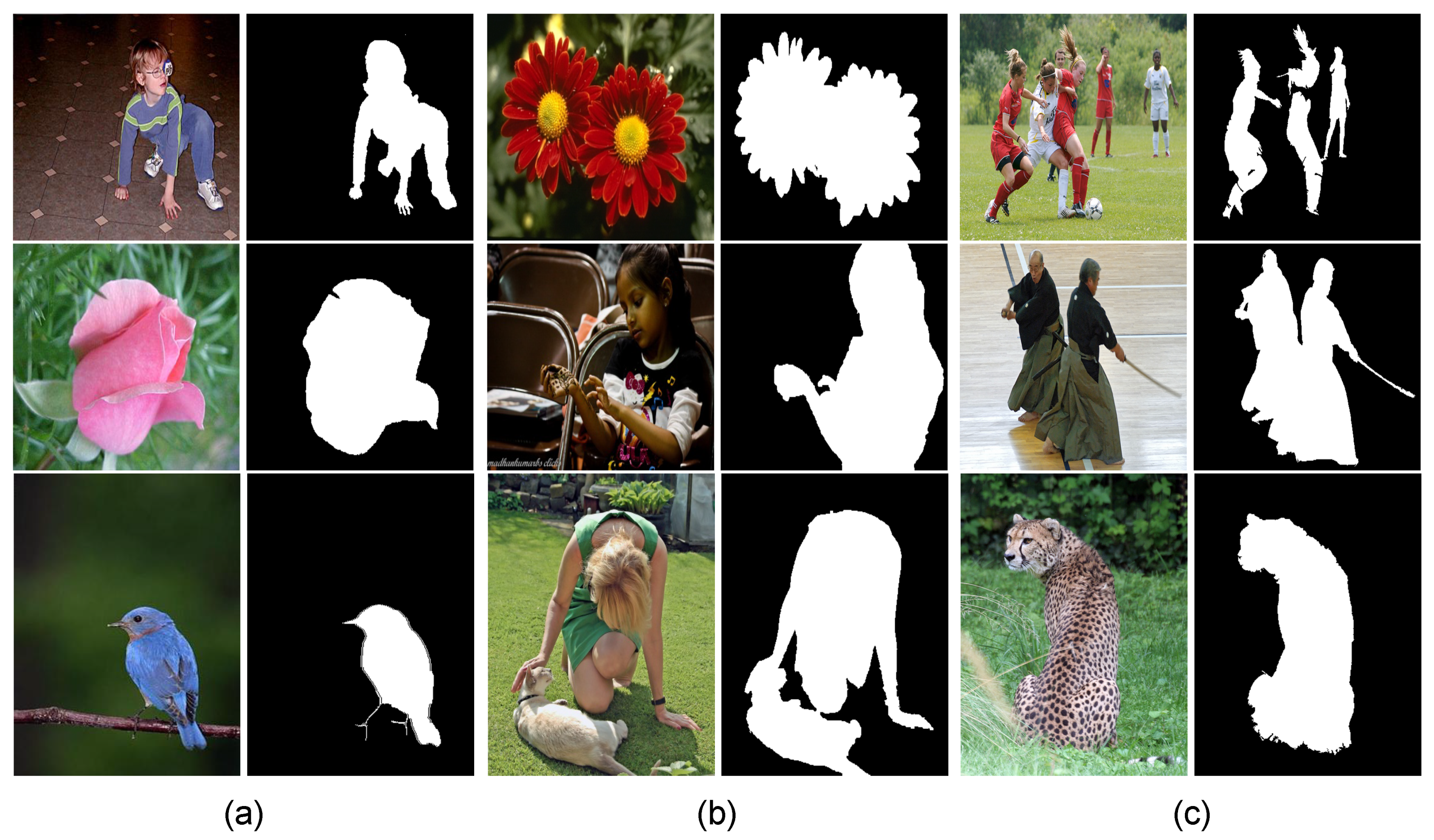
In this work, we used three benchmark datasets typically used to evaluate the performance of salient object detection methods: MSRA1K [15], ECSSD [46], and iCoseg [47]. We used such datasets since they have been used in diverse research works, such as those by Borji et al. [48], and Jiang et al. [49], containing one or multiple salient objects under complex scenarios. Furthermore, the ground truth is available and given at the pixel level. The MSRA1K [15] dataset contains 1000 images with unambiguous salient objects under a diversity of scenes, with the binary annotations at the pixel level. ECSSD [46] dataset includes 1000 images with the binary pixel-wise annotations of the salient object. This dataset contains images mainly of natural scenarios with a cluttered background. The iCoseg [47] dataset includes 643 images of a wide variety of scenarios. In addition, this dataset includes the binary pixel-wise segmentation of one or multiple salient objects present in the images. The object segmentation was done by a human user. In Figure 4, we show three sample images of each database and their corresponding ground truth.
For a quantitative evaluation of the RSD method performance, we adopted, in the evaluation setup, the F-measure metric. Originally, the F-measure was introduced for evaluation of information extraction technology [50]. The F-measure is frequently used to measure performance in a variety of prediction problems [51], such as binary classification and multi-label classification. Considering saliency detection as a binary classification task, the F-measure has been adopted by diverse authors to evaluate saliency detection models.
The F-measure depends on two metrics: precision and recall. In the saliency detection task, the precision value is defined as the ratio of correctly assigned salient pixels and the total number of salient pixels predicted, while the recall is defined as the proportion of detected salient pixels and the total number of salient pixels according to the ground truth. The precision and recall are defined as in Equations (13) and (14), respectively.
p r e c i s i o n = t r u e _ p o s i t i v e t r u e _ p o s i t i v e + f a l s e _ p o s i t i v e ,
r e c a l l = t r u e _ p o s i t i v e t r u e _ p o s i t i v e + f a l s e _ n e g a t i v e .
The F-measure is defined as the weighted harmonic mean of precision and recall metrics, with a non-negative weight of β . In Equation (15) we give the formulation of F-measure.
F β = ( 1 + β 2 ) p r e c i s i o n × r e c a l l β 2 × p r e c i s i o n + r e c a l l ,
where β is a parameter to control the weight of precision and recall metrics. Following the arguments presented by Borji et al. [48], where it is stated that precision is more important than recall, and in a similar manner as in Achanta et al. [15], we set β 2 with a fixed value of 0.3 to weight precision more than recall.

3.2. Parameter Setting

The proposed model makes use of a learning algorithm. In our case, we used the MODLEM algorithm, whose implementation can be found at WEKA repository. The MODLEM algorithm implementation at WEKA offers certain parameters that can be selected according to the needs of the user. The parameters needed are: rules type generation, condition of measure, classification strategy, and matching type. To avoid any uncertainty, we selected the lower approximation as the rules type. Preliminary tests were carried out varying the conditions of measure, and those empiric tests led us to select the Laplace estimator. The nearest rule was selected as the classification strategy and the matching type was selected as full matching type.

3.3. Evaluation

To calculate the performance of our proposal, we compared RSD against seven state-of-the-art approaches: Minimum Barrier Salient (MBS) [40], Minimum Directional Contrast (MDC) [25], Saliency Filters (SF) [23], Histogram-Contrast and Region-Contrast (HC, RC) [22], Frequency-Tuned (FT) [15], and Context-Aware (CA) [24]. In addition, we considered for comparison purposes a learning-based aggregation model such as Pixel-Wise (PW) [28]. For a fair comparison, the PW model learns from the same feature descriptors proposed for our RSD approach.
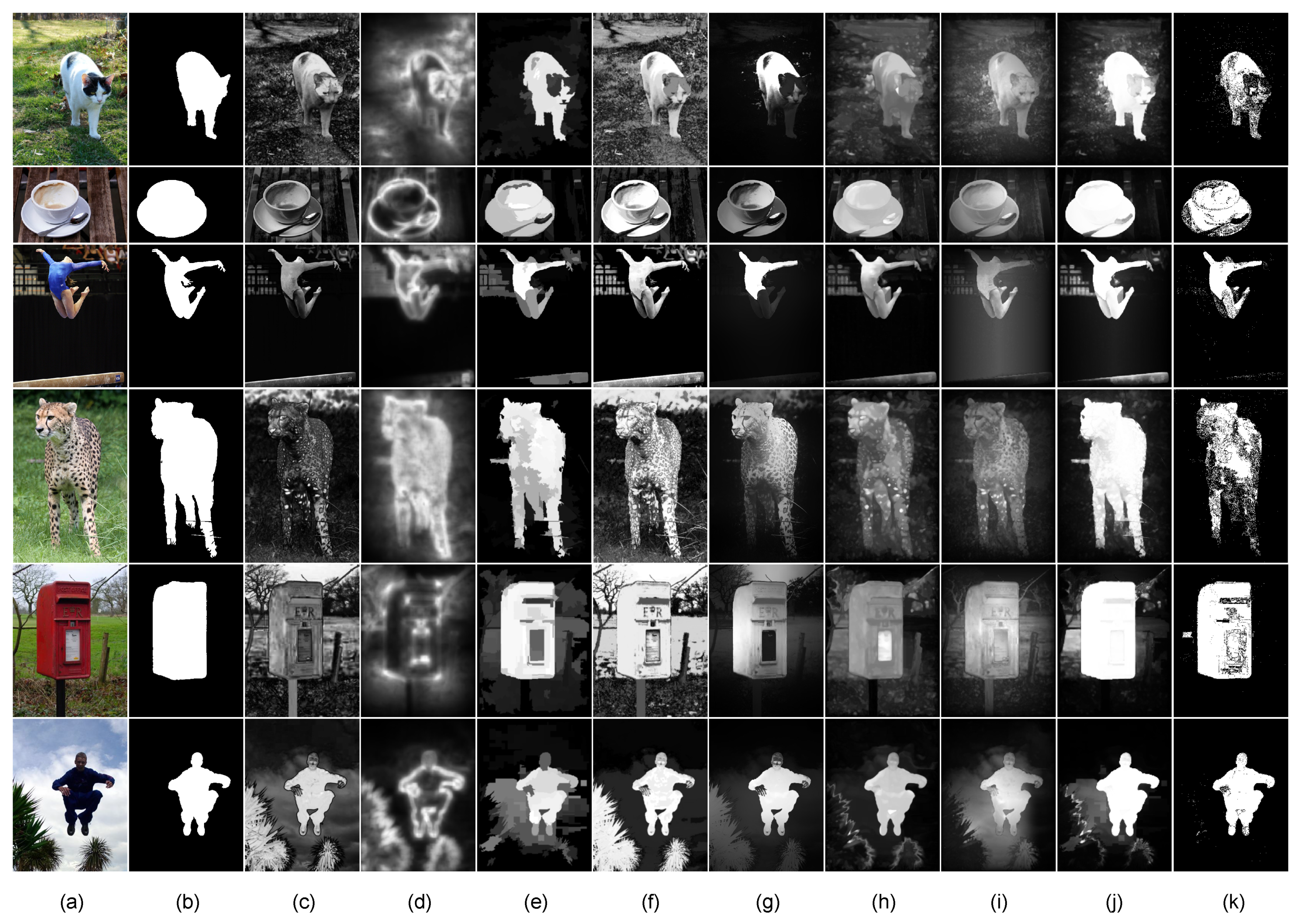
In Figure 5, we present samples of the binary map obtained by our RSD and the saliency maps from the methods used for comparison purposes. In this figure, we can observe that the saliency maps obtained by individual and aggregation methods are given in a grayscale image. Conversely, the saliency map obtained from our proposed system is given as a binary map.
Considering that there is not an optimal threshold to use with each individual method, our evaluation approach was twofold. In our first experiment, we used one of the most common methods to automatically obtain the best threshold and to evaluate all the methods under the same specification. Specifically, we utilized the adaptive threshold [15], which is one of the most popular methods used for image saliency and it is simple to calculate. The adaptive threshold is defined in Equation (16).
T a = 2 W × H x = 1 W y = 1 H S ( x , y ) ,
where W and H are the width and height of the saliency map image, respectively, and S ( x , y ) is the saliency level of the outcome inspected. In our second experiment, to evaluate all the methods under their best specific conditions, we obtained the binary result of the saliency maps with all possible thresholds in the range of [ 0 , 255 ] . In both experiments, we adopted a cross-validation method to estimate the performance of our proposed approach with five folds.

3.3.1. Comparison of Diverse Combinations

In this section, we present the procedure to determine the best set of saliency models to be used as input features by our system. We combined the candidate saliency models incrementally following two strategies, from best to worst model and from worst to best model, resulting in thirteen representative combinations. In Table 1, we list the performance of the seven candidate saliency models on the iCoseg dataset by ranking the F-measure.
In Table 2, we present the F-measure performance obtained on the iCoseg dataset by each considered combination. The best performance is highlighted in bold. The evaluation and analysis of the two combination strategies are detailed below.
Superior ranked models aggregation In the first combination strategy, we aggregated models incrementally, from the model with the best performance to the model with the worst performance. That is, we selected the best saliency model for the first test, the two best saliency models for the second test and so forth. The results presented in Table 2 indicate that the combination that obtained the better performance in F-measure metric includes the four better models RC, SF, MDC, and MBS.
Inferior ranked models aggregation In the second combination strategy, we aggregated models, from the lowest performance model to the highest performance model. Thus, we utilized the worst performance model for the first test, the two worst performance models for the second test and so forth. In Table 2, we can notice that the combination that obtained the best performance includes the models CA, HC, FT, MBS, MDC, and SF.
According to the results depicted in Table 2, the best combination of inferior models performed lower than the best combination of superior models. In general, the best performance was achieved by aggregating the superior models. In view of the obtained results from the two combination strategies, we selected the models RC, SF, MDC, and MBS as input features of our system. In fact, the highest score was obtained by the combination including two models that estimate saliency in a region-based manner and two models that compute saliency in a pixel-wise manner. Additionally, the four models utilize the CIELAB color space.

3.3.2. Saliency Detection Comparison Using an Adaptive Threshold

In our first experiment, we performed a comparison of the proposed RSD method and other methods on each dataset. To compute precision, recall, and F-measure, we needed to binarize the saliency maps from saliency models. We binarized the maps obtained from individual methods by using the adaptive threshold.From each binarized image, we computed precision, recall, and F-measure metrics. The overall performance on each dataset was estimated by averaging these metrics obtained from each image.
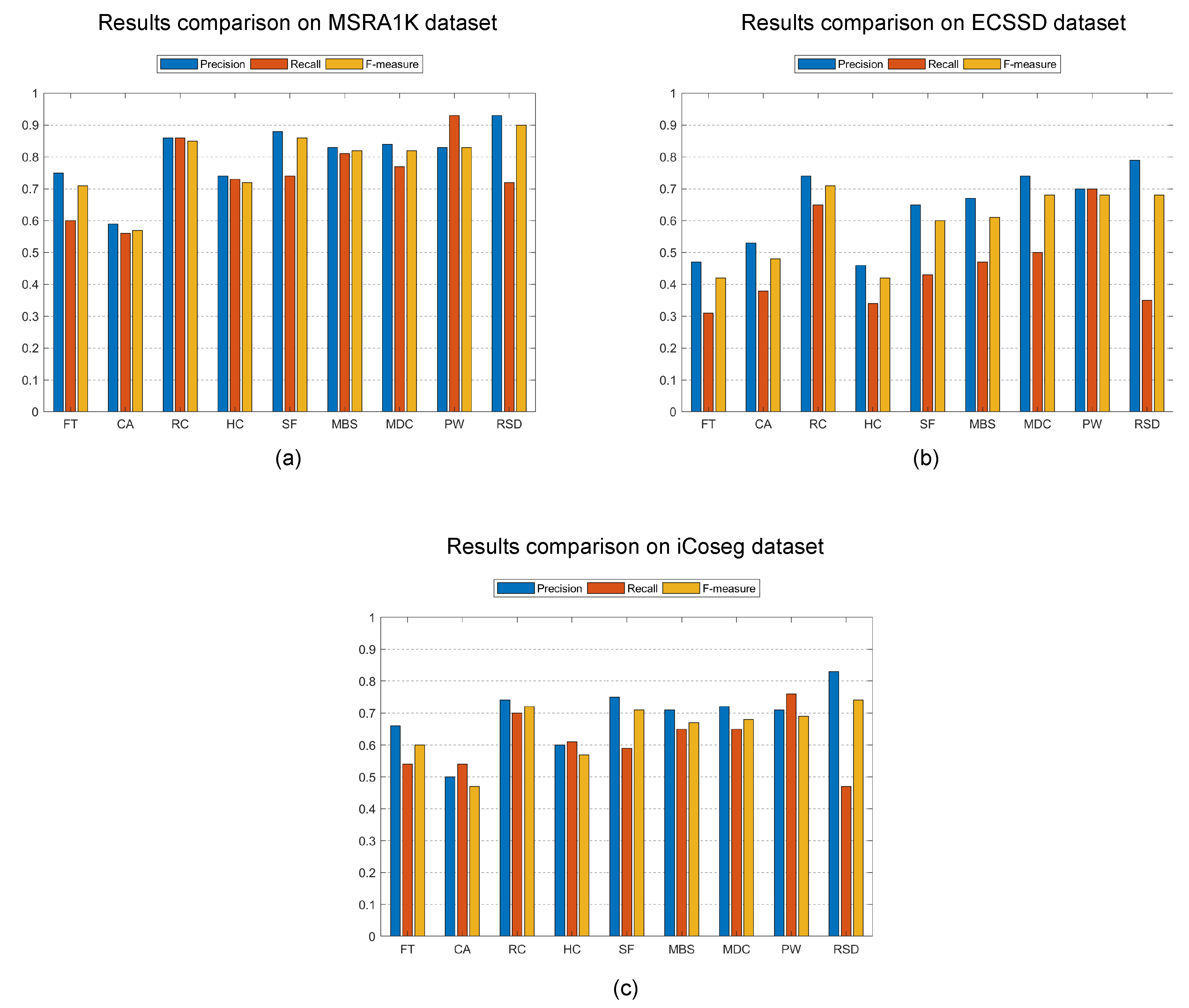
The obtained results on the three datasets are depicted in Figure 6. In the MSRA1K dataset, our RSD model outperformed other models; the F-Measure obtained by our model was 0.897 while the SF model, which is the most proximate model, obtained 0.858. The highest precision value was achieved by our approach, which scored 0.929, while the most proximate model, SF, obtaind a precision value of 0.879. The recall measure obtained by our model was 0.723, and the PW model attained the highest recall measure of 0.927.
From the results obtained on iCoseg dataset, we observed that our proposal obtained an F-measure value of 0.736, whereas the model RC achieved 0.717. Our proposal obtained the highest precision value of 0.826 while the SF model performed 0.749. The PW model obtained the highest recall value of 0.756. Finally, the results obtained in ECSSD dataset indicate that the RC model obtained the highest F-measure value of 0.708, while our approach scored 0.679. In contrast, our proposal attained the highest precision value of 0.789 while the RC model achieved a precision value of 0.738. The PW model obtained the highest recall measure of 0.700.
In Table 3, we present the overall performance of our RSD model and the rest of the models by averaging the results obtained from the adaptive thresholding test on the three datasets used. As shown in the table, our proposal obtained the highest F-measure of 0.770. In the case of the precision metric, the proposed model obtained the highest precision performance of 0.847. The RC model attained 0.759 and 0.780 for F-measure and precision, respectively. The highest recall of 0.794 was obtained by PW model, whereas our model performed 0.513. The model that obtained the highest score on each metric is highlighted in bold.
It is worth mentioning that, according to Liu et al. [52], recall measure is not a meaningful metric in saliency prediction task. Liu claimed that a 100% recall can be achieved by choosing all image locations as salient. The challenging task of any saliency detection model should be to detect with high accuracy, the salient locations into a visual scene.
The obtained results indicate that, even though the outcomes from aggregation and individual models are binarized by using their best threshold, our proposed RSD model performed better, without the need of looking for the best threshold.

3.3.3. Saliency Detection Comparison with All Thresholds

As mentioned above, in our second experiment, to evaluate all the methods under their best specific conditions, we obtained the binary result of the saliency maps with all possible thresholds in the range of [ 0 , 255 ] . Results of the second experiment are shown in Figure 7. In this figure, the horizontal-axis corresponds to the threshold value and the vertical-axis corresponds to the F-measure resulting from the use of the given threshold. Since our method RSD does not need a post-processing/thresholding step, the F-measure is the same for all possible thresholds. As shown in this figure, other methods reached maximum performance in a bounded range of the threshold values. In contrast, the solution of the proposed approach showed a constant performance due to thresholding independence.
In the MSRA1K dataset (Figure 7a), our RSD achieved a maximum and steady F-measure value of 0.896 while the PW model reached a maximum value of 0.910 in a bounded range. The RC and PW models slightly overcame the proposed model in ECSSD and iCoseg datasets, as presented in Figure 7b,c, respectively. These models obtained higher F-measure values in a bounded range. In the ECSSD dataset the RC and PW obtained 0.726 and 0.747, respectively, and our proposal achieved 0.679. On the other hand, in the iCoseg dataset, our model attained 0.735 while the RC and PW achieved 0.765 and 0.775, respectively.
In Table 4, we present the average F-measure from all the computed values on each threshold. In this table, we can observe that the average result of our proposed RSD performed higher than the rest of the models on the three datasets used. The model with the highest performance is highlighted in bold.
The maximum F-measure rate reached at the curve by individual and aggregation models occured in a bounded threshold range. This aspect of the behavior of the models produced a peak when plotting the F-measure curve. An ascending and descending slope is the typical shape observed of the F-measure curve, which implies that there exist threshold values where the performance of the model is minimum. In contrast, the binary outcome produced by the RSD model maintained the same performance across the whole threshold range. The results obtained point out that the outcome from our RSD model performed steadily, being insensitive to the threshold. In contrast, the individual and aggregation models achieved their best performance at a certain range of threshold values, which was a bounded and ambiguous range. The output obtained from our RSD model gave us the certainty of constant performance.

4. Conclusions

In this paper, we present a rule-based approach for saliency detection. In our method, features are learned automatically using a rough-set-based approach. Our rule-based system provides a practical tool for building automated methods where high performance is required. The contribution of this paper is twofold. Firstly, we extract salient information from an image and our method automatically decodes the knowledge found in each individual model and combines the four features in a useful way. The use of a rough-set-based approach allows our RSD system to represent the characteristics of saliency using a simple set of rules. Besides, the output obtained from our proposal is given in a binary manner, where each pixel position is evaluated as salient or not, eliminating any uncertainty. Therefore, the second contribution of our proposal eliminates the need to implement any post-processing to obtain a binary saliency map. The evaluation of the proposed method was carried out with experiments on real datasets. Quantitative results show that our method is robust and flexible in finding the salient pixels within an image, is not threshold dependant and is more accurate than other state-of-the-art methods.

Author Contributions

Conceptualization, R.E.S.-Y.; Investigation, A.L.-A.; Project administration, R.A.L.-M.; and Software, D.E.M.-R. and M.A.C.-C.

Funding

This research received no external funding.

Conflicts of Interest

The authors declare no conflict of interest with respect to this study.

References

  1. Koch, C.; Ullman, S. Shifts in selective visual attention: Towards the underlying neural circuitry. Hum. Neurobiol. 1985, 4, 219–227. [Google Scholar] [PubMed]
  2. Guo, C.; Zhang, L. A novel multiresolution spatiotemporal saliency detection model and its applications in image and video compression. IEEE Trans. Image Process. 2010, 19, 185–198. [Google Scholar]
  3. Stentiford, F. An estimator for visual attention through competitive novelty with application to image compression. In Proceedings of the Picture Coding Symposium 2001, Seoul, Korea, 25–27 April 2001; pp. 101–104. [Google Scholar]
  4. Ouerhani, N.; Bracamonte, J.; Hügli, H.; Ansorge, M.; Pellandini, F. Adaptive color image compression based on visual attention. In Proceedings of the 11th International Conference on Image Analysis and Processing, Palermo, Italy, 26–28 September 2001; Volume 11, pp. 416–421. [Google Scholar]
  5. Ren, Z.; Gao, S.; Chia, L.; Tsang, I.W. Region-based saliency detection and its application in object recognition. IEEE Trans. Circuits Syst. Video Technol. 2014, 24, 769–779. [Google Scholar] [CrossRef]
  6. Gao, D.; Han, S.; Vasconcelos, N. Discriminant saliency, the detection of suspicious coincidences, and applications to visual recognition. IEEE Trans. Pattern Anal. Mach. Intell. 2009, 31, 989–1005. [Google Scholar]
  7. Rutishauser, U.; Walther, D.; Koch, C.; Perona, P. Is bottom-up attention useful for object recognition? In Proceedings of the 2004 IEEE Computer Society Conference on Computer Vision and Pattern Recognition, 2004. CVPR 2004, Washington, DC, USA, 27 June–2 July 2004. [Google Scholar]
  8. Mei, T.; Hua, X.S.; Yang, L.; Li, S. VideoSense: Towards effective online video advertising. In Proceedings of the 15th ACM international conference on Multimedia, Augsburg, Germany, 25–29 September 2007; pp. 1075–1084. [Google Scholar]
  9. Chang, C.H.; Hsieh, K.Y.; Chung, M.C.; Wu, J.L. ViSA: Virtual spotlighted advertising. In Proceedings of the 16th ACM international conference on Multimedia, Vancouver, BC, Canada, 26–31 October 2008; pp. 837–840. [Google Scholar]
  10. 3M. Visual Attention System (VAS). Available online: https://www.3m.com/3M/en_US/visual-attention-software-us (accessed on 3 October 2018).
  11. Frintrop, S.; Jensfelt, P. Attentional landmarks and active gaze control for visual SLAM. IEEE Trans. Robot. 2008, 24, 1054–1065. [Google Scholar] [CrossRef]
  12. Siagian, C.; Itti, L. Biologically inspired mobile robot vision localization. IEEE Trans. Robot. 2009, 25, 861–873. [Google Scholar] [CrossRef]
  13. Chang, C.; Siagian, C.; Itti, L. Mobile robot vision navigation & localization using Gist and Saliency. In Proceedings of the 2010 IEEE/RSJ International Conference on Intelligent Robots and Systems, Taipei, Taiwan, 18–22 October 2010; pp. 4147–4154. [Google Scholar]
  14. Borji, A.; Sihite, D.N.; Itti, L. Salient object detection: A benchmark. In Proceedings of the European Conference on Computer Vision, (ECCV), Florence, Italy, 7–13 October 2012; pp. 414–429. [Google Scholar]
  15. Achanta, R.; Hemami, S.; Estrada, F.; Susstrunk, S. Frequency-tuned salient region detection. In Proceedings of the IEEE International Conference on Computer Vision and Pattern Recognition (CVPR 2009), Miami Beach, FL, USA, 20–25 June 2009; pp. 1597–1604. [Google Scholar]
  16. Itti, L.; Koch, C.; Niebur, E. A model of saliency-based visual attention for rapid scene analysis. IEEE Trans. Pattern Anal. Mach. Intell. 1998, 20, 1254–1259. [Google Scholar] [CrossRef] [Green Version]
  17. Treisman, A.M.; Gelade, G. A feature-integration theory of attention. Cogn. Psychol. 1980, 12, 97–136. [Google Scholar] [CrossRef]
  18. Frintrop, S.; Klodt, M.; Rome, E. A real-time visual attention system using integral images. In Proceedings of the 5th International Conference on Computer Vision Systems, Bielefeld, Germany, 21–24 March 2007; pp. 1–10. [Google Scholar]
  19. Frintrop, S.; Werner, T.; Garcia, G.M. Traditional saliency reloaded: A good old model in new shape. In Proceedings of the 2015 IEEE Conference on Computer Vision and Pattern Recognition (CVPR), Boston, MA, USA, 7–12 June 2015; pp. 82–90. [Google Scholar]
  20. Parkhurst, D.; Law, K.; Niebur, E. Modeling the role of salience in the allocation of overt visual attention. Vis. Res. 2002, 42, 107–123. [Google Scholar] [CrossRef] [Green Version]
  21. Le Meur, O.; Le Callet, P.; Barba, D.; Thoreau, D. A coherent computational approach to model the bottom-up visual attention. IEEE Trans. Pattern Anal. Mach. Intell. 2006, 28, 802–817. [Google Scholar] [CrossRef] [PubMed]
  22. Cheng, M.M.; Mitra, N.J.; Huang, X.; Torr, P.H.S.; Hu, S.M. Global contrast based salient region detection. IEEE Trans. Pattern Anal. Mach. Intell. 2015, 37, 569–582. [Google Scholar] [CrossRef] [PubMed]
  23. Perazzi, F.; Krahenbuhl, P.; Pritch, Y.; Hornung, A. Saliency filters: Contrast based filtering for salient region detection. In Proceedings of the 2012 IEEE Conference on Computer Vision and Pattern Recognition, Providence, RI, USA, 16–21 June 2012; pp. 733–740. [Google Scholar]
  24. Goferman, S.; Zelnik-Manor, L.; Tal, A. Context-aware saliency detection. IEEE Trans. Pattern Anal. Mach. Intell. 2012, 34, 1915–1926. [Google Scholar] [CrossRef] [PubMed]
  25. Huang, X.; Zhang, Y.J. 300-FPS salient object detection via minimum directional Contrast. IEEE Trans. Image Process. 2017, 26, 4243–4254. [Google Scholar] [CrossRef] [PubMed]
  26. Itti, L.; Koch, C. Computational modelling of visual attention. Nat. Rev. Neurosci. 2001, 2, 194–203. [Google Scholar] [CrossRef]
  27. Bylinskii, Z.; Judd, T.; Oliva, A.; Torralba, A.; Durand, F. What do different evaluation metrics tell us about saliency models? IEEE Trans. Pattern Anal. Mach. Intell. 2019, 41, 740–757. [Google Scholar] [CrossRef]
  28. Mai, L.; Niu, Y.; Liu, F. Saliency aggregation: A data-driven approach. In Proceedings of the 2013 IEEE Conference on Computer Vision and Pattern Recognition (CVPR), Portland, OR, USA, 23–28 June 2013; pp. 1131–1138. [Google Scholar]
  29. Wang, L.; Lu, H.; Ruan, X.; Yang, M.H. Deep networks for saliency detection via local estimation and global search. In Proceedings of the 2015 IEEE Conference on Computer Vision and Pattern Recognition (CVPR), Boston, MA, USA, 7–12 June 2015; pp. 3183–3192. [Google Scholar]
  30. Zhao, R.; Ouyang, W.; Li, H.; Wang, X. Saliency detection by multi-context deep learning. In Proceedings of the 2015 IEEE Conference on Computer Vision and Pattern Recognition (CVPR), Boston, MA, USA, 7–12 June 2015; pp. 1265–1274. [Google Scholar]
  31. Liu, N.; Han, J. DHSNet: Deep hierarchical saliency network for salient object Detection. In Proceedings of the 2016 IEEE Conference on Computer Vision and Pattern Recognition (CVPR), Las Vegas, NV, USA, 27–30 June 2016; pp. 678–686. [Google Scholar]
  32. Hu, P.; Shuai, B.; Liu, J.; Wang, G. Deep level sets for salient object detection. In Proceedings of the 2017 IEEE Conference on Computer Vision and Pattern Recognition (CVPR), Honolulu, HI, USA, 21–26 July 2017; pp. 540–549. [Google Scholar]
  33. Chen, S.; Wang, B.; Tan, X.; Hu, X. Embedding attention and residual network for accurate salient object detection. IEEE Trans. Cybern. 2018. [Google Scholar] [CrossRef]
  34. Napierala, K.; Stefanowski, J. BRACID: A comprehensive approach to learning rules from imbalanced data. J. Intell. Inf. Syst. 2012, 39, 335–373. [Google Scholar] [CrossRef]
  35. Stefanowski, J. On Combined Classifiers, Rule Induction and Rough Sets. Trans. Rough Sets VI LNCS 2007, 4374, 329–350. [Google Scholar]
  36. Pawlak, Z. Rough sets. Int. J. Comput. Inf. Sci. 1982, 11, 341–356. [Google Scholar] [CrossRef]
  37. Swiniarski, R. Rough sets methods in feature reduction and classification. Int. J. Appl. Math. Comput. Sci. 2001, 11, 565–582. [Google Scholar]
  38. Tay, F.E.; Shen, L. Economic and financial prediction using rough sets model. Eur. J. Oper. Res. 2002, 141, 641–659. [Google Scholar] [CrossRef] [Green Version]
  39. Pawlak, Z. Why rough sets? Proc. IEEE Int. Fuzzy Syst. 1996, 2, 738–743. [Google Scholar]
  40. Zhang, J.; Sclaroff, S.; Lin, Z.; Shen, X.; Price, B.; Mech, R. Minimum barrier salient object detection at 80 FPS. In Proceedings of the 2015 IEEE Conference on Computer Vision and Pattern Recognition (ICCV), Santiago, Chile, 11–18 December 2015; pp. 1404–1412. [Google Scholar]
  41. Stefanowski, J. On rough set based approaches to induction of decision rules. Rough Sets Knowl. Discov. 1998, 1, 500–529. [Google Scholar]
  42. Stefanowski, J. The rough set based rule induction technique for classification problems. In Proceedings of the 6th European Conference on Intelligent Techniques and Soft Computing EUFIT, Aachen, Germany, 7–10 September 1998; Volume 98, pp. 109–113. [Google Scholar]
  43. Grzymala-Busse, J.W.; Stefanowski, J. Three discretization methods for rule induction. Int. J. Intell. Syst. 2001, 16, 29–38. [Google Scholar] [CrossRef]
  44. Hall, M.; Frank, E.; Holmes, G.; Pfahringer, B.; Reutemann, P.; Witten, I.H. The WEKA data mining software: An update. ACM SIGKDD Explor. Newsl. 2009, 11, 10–18. [Google Scholar] [CrossRef]
  45. Rother, C.; Kolmogorov, V.; Blake, A. GrabCut: Interactive foreground extraction using iterated graph cuts. ACM Trans. Graph. 2004, 23, 309–314. [Google Scholar] [CrossRef]
  46. Shi, J.; Yan, Q.; Xu, L.; Jia, J. Hierarchical image saliency detection on extended CSSD. IEEE Trans. Pattern Anal. Mach. Intell. 2016, 38, 717–729. [Google Scholar] [CrossRef]
  47. Batra, D.; Kowdle, A.; Parikh, D.; Luo, J.; Chen, T. iCoseg: Interactive co-segmentation with intelligent scribble guidance. In Proceedings of the 2010 IEEE Computer Society Conference on Computer Vision and Pattern Recognition, San Francisco, CA, USA, 13–18 June 2010; pp. 3169–3176. [Google Scholar]
  48. Borji, A.; Cheng, M.M.; Jiang, H.; Li, J. Salient object detection: A benchmark. IEEE Trans. Image Process. 2015, 24, 5706–5722. [Google Scholar] [CrossRef]
  49. Jiang, H.; Wang, J.; Yuan, Z.; Wu, Y.; Zheng, N.; Li, S. Salient object detection: A discriminative regional feature integration approach. In Proceedings of the IEEE Conference on Computer Vision and Pattern Recognition (CVPR), Portland, OR, USA, 23–28 June 2013; pp. 2083–2090. [Google Scholar]
  50. Powers, D.M.W. Evaluation: From precision, recall and f-factor to roc, informedness, markedness and correlation. J. Mach. Learn. Technol. 2011, 2, 37–63. [Google Scholar]
  51. Dembczynski, K.J.; Waegeman, W.; Cheng, W.; Hüllermeier, E. An exact algorithm for f-measure maximization. In Advances in Neural Information Processing Systems; Curran Associates, Inc.: Red Hook, NY, USA, 2011; pp. 1404–1412. [Google Scholar]
  52. Liu, T.; Yuan, Z.; Sun, J.; Wang, J.; Zheng, N.; Tang, X.; Shum, H. Learning to Detect a Salient Object. IEEE Trans. Pattern Anal. Mach. Intell. 2011, 33, 353–367. [Google Scholar] [PubMed]
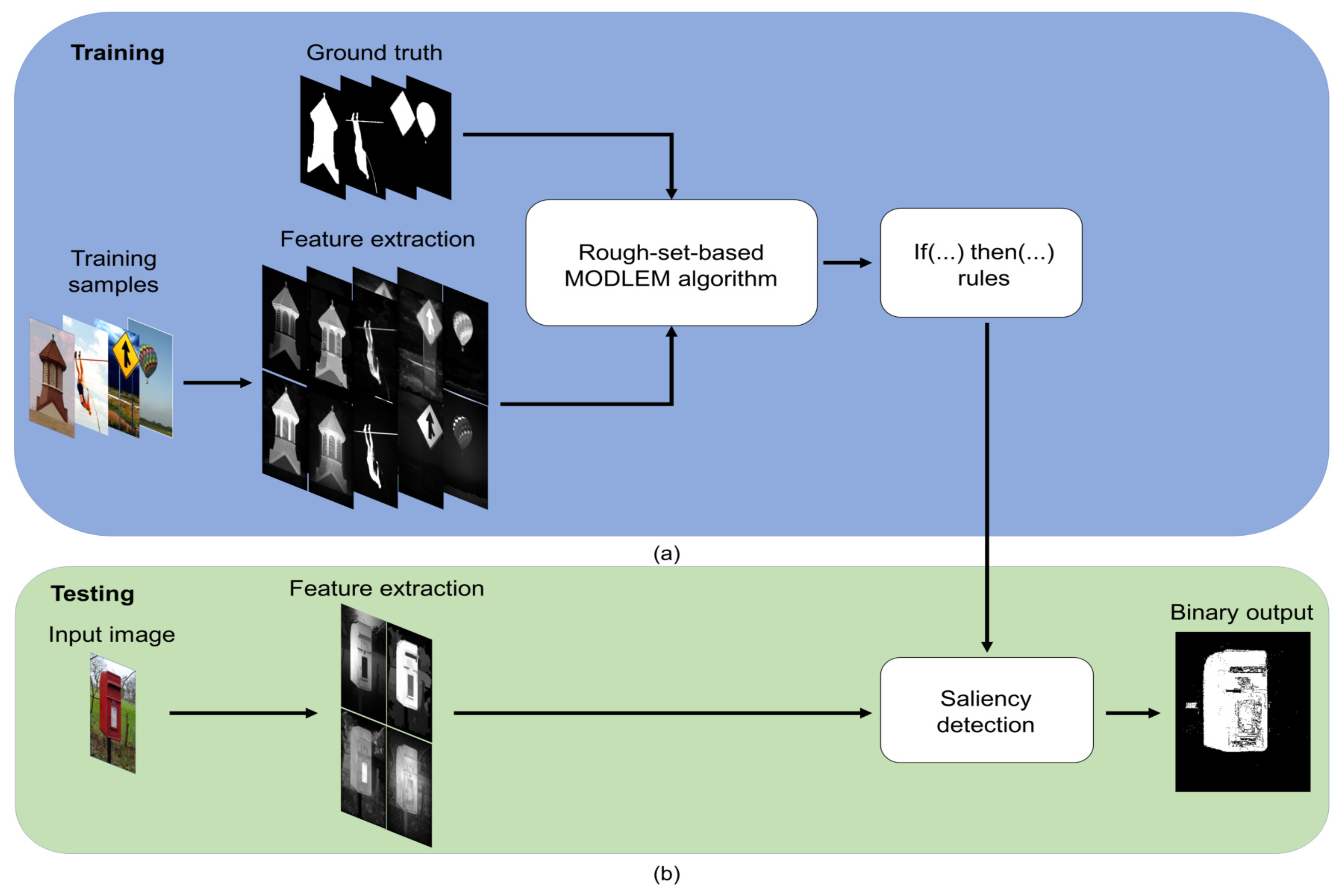
Figure 1. Overview of our proposed model. (a) Feature extraction is performed. Then, a learning process is carried out by using the MODLEM algorithm. (b) Using the obtained model, a saliency prediction is performed and the output is given in a binary form.
Applsci 09 02015 g001
Figure 2. Illustration of the training stage. Firstly, saliency maps are computed. Secondly, sampling is carried out by using labeled annotations from ground truth. Then, the learning step is performed by the MODLEM algorithm and the result is a rule-based saliency detection model.
Applsci 09 02015 g002
Figure 3. Ten samples out of the complete set of rules obtained from MODLEM algorithm.
Applsci 09 02015 g003
Figure 4. Three sample images of each dataset used and their corresponding ground truth: (a) MSRA1K dataset; (b) ECSSD dataset; and (c) iCoseg dataset.
Applsci 09 02015 g004
Figure 5. Saliency maps of individual and aggregation methods. The binary outcome obtained from our approach is presented: (a) Input image; (b) Ground truth; (c) FT; (d) CA; (e) RC; (f) HC; (g) SF; (h) MBS; (i) MDC; (j) PW; and (k) RSD.
Applsci 09 02015 g005
Figure 6. Precision, Recall, and F-measure metrics obtained from the binarized outcomes of the methods: (a) MSRA1K dataset; (b) ECSSD dataset; and (c) iCoseg dataset.
Applsci 09 02015 g006
Figure 7. Comparison of the F-measure curve obtained with different thresholds for eight state-of-the-art algorithms and our approach RSD on three representative benchmark datasets: (a) MSRA1K dataset; (b) ECSSD dataset; and (c) iCoseg dataset.
Applsci 09 02015 g007
Table 1. The list of models ranked by their F-measure. The individual models are ranked according to the obtained F-measure on the iCoseg dataset from higher to lower score.
MethodF-Measure
RC (2011)0.720
SF (2012)0.707
MDC (2017)0.680
MBS (2015)0.665
FT (2009)0.601
HC (2011)0.572
CA (2010)0.467
Table 2. Performance comparison of various saliency models combinations. The combination that includes the RC, SF, MDC, and MBS models obtains the better performance in F-measure score.
Superior
CombinationF-Measure
RC0.633
RC, SF0.663
RC, SF, MDC0.715
RC, SF, MDC, MBS0.736
RC, SF, MDC, MBS, FT0.730
RC, SF, MDC, MBS, FT, HC0.726
RC, SF, MDC, MBS, FT, HC, CA0.725
Inferior
CombinationF-Measure
CA0.191
CA, HC0.547
CA, HC, FT0.566
CA, HC, FT, MBS0.644
CA, HC, FT, MBS, MDC0.667
CA, HC, FT, MBS, MDC, SF0.687
Table 3. Average performance on the three datasets used. The model with the highest performance on each metric is highlighted in bold.
MethodAverage F-MeasureAverage PrecisionAverage Recall
FT (2009)0.5770.6240.481
CA (2010)0.5050.5400.489
RC (2011)0.7590.7800.737
HC (2011)0.5720.5990.559
SF (2012)0.7220.7600.589
PW (2013)0.7340.7440.794
MBS (2015)0.6990.7360.642
MDC (2017)0.7260.7650.640
RSD (ours)0.7700.8470.513
Table 4. The averaged F-measure of the results obtained on each fixed threshold. The model with the highest performance is highlighted in bold.
Method (year)MSRA1KECSSDiCoseg
F-MeasureF-MeasureF-Measure
AverageAverageAverage
FT (2009)0.4810.2800.434
CA (2010)0.4390.3740.407
RC (2011)0.7610.6280.675
HC (2011)0.6520.3880.553
SF (2012)0.7330.4890.611
PW (2013)0.8160.6370.677
MBS (2015)0.5960.4150.516
MDC (2017)0.5840.4470.515
RSD (ours)0.8960.6790.735