Framework for Fast Experimental Testing of Autonomous Navigation Algorithms

Abstract

Research in mobile robotics requires fully operative autonomous systems to test and compare algorithms in real-world conditions. However, the implementation of such systems remains to be a highly time-consuming process. In this work, we present an robot operating system (ROS)-based navigation framework that allows the generation of new autonomous navigation applications in a fast and simple way. Our framework provides a powerful basic structure based on abstraction levels that ease the implementation of minimal solutions with all the functionalities required to implement a whole autonomous system. This approach helps to keep the focus in any sub-problem of interest (i.g. localization or control) while permitting to carry out experimental tests in the context of a complete application. To show the validity of the proposed framework we implement an autonomous navigation system for a ground robot using a localization module that fuses global navigation satellite system (GNSS) positioning and Monte Carlo localization by means of a Kalman filter. Experimental tests are performed in two different outdoor environments, over more than twenty kilometers. All the developed software is available in a GitHub repository.

1. Introduction

Autonomous navigation is currently one of the more important topics in robotics since robots capable of moving freely in their environments can produce a large number of new applications in many fields, like logistics [1], agriculture [2] or passenger transport [3]. There are researches covering this topic since the nineteen-seventies [4], so it is a mature field with lots of published algorithms and available tools. In addition, recent advances like the emergence of deep learning are providing researchers with very advanced scene understanding algorithms [5,6]. However, real applications in real conditions—especially in outdoor environments—remain to be a challenge [7].

The usual architecture of an autonomous navigation system—whether it be terrestrial, marine or aerial—relies on the use of several dedicated subsystems, that solve different required tasks like localization [8,9], mapping, path-planning, and control, among others [10,11,12]. Each one of these tasks belongs to different research topics making mobile robotics an extremely interdisciplinary field [13]. One approach to cope with this complexity is to study the different subsystems separately, what simplifies—and reduces the costs of—the experimental processes. For instance, localization algorithms can be developed making use of public datasets [14], and researchers in control can take advantage of robotic simulators to develop their algorithms [15]. However, these approaches are not sufficient to make a comprehensive evaluation of the developed algorithms, because real systems present interactions—and even feedbacks—between their different modules whose effects can only be observed when the whole system is implemented and tested in real-world conditions [16]. Only extensive experimental tests spanning different conditions and environments can bring enough information for a comprehensive system evaluation. Moreover, these kinds of tests are extremely useful to guide the development processes in a robust and productive way. In the present paper, we introduce a robotic operating system (ROS)-based navigation framework that provides a powerful basic structure based on abstraction levels. This framework is designed to generate minimal but complete autonomous navigation solutions, thus speeding-up the implementation processes required to obtain a full system suitable for experimental testing. This approach permits to save efforts and to keep the focus in concrete research problems, without the drawbacks of simulators and datasets. To show that our framework can be an excellent tool to test and compare different algorithms, we first implement a fully operative autonomous navigation system and then we show how easy results to modify it. Concretely, we change its initial 2D simultaneous localization and mapping (SLAM) localization module by a new one that implements a loosely coupled architecture integrating global navigation satellite system GNSS information and 2D SLAM by means of a Kalman filter. Thanks to this GNSS fusion approach our ground vehicle is able to navigate autonomously in the University of Alicante campus, going in and out from the mapped area. This mixed on-map/off-map navigation is straightforward using our framework, but it would have been very hard to implement using the existing alternatives, as explained later. The system has been evaluated through three experimental sessions, in two different environments, with two different localization algorithms, accumulating more than twenty kilometers of navigation in real-world conditions. Summarizing, our contributions are the following (All the software described in this paper is publicly available and can be found in a GitHub repository https://github.com/AUROVA-LAB/aurova_framework.):

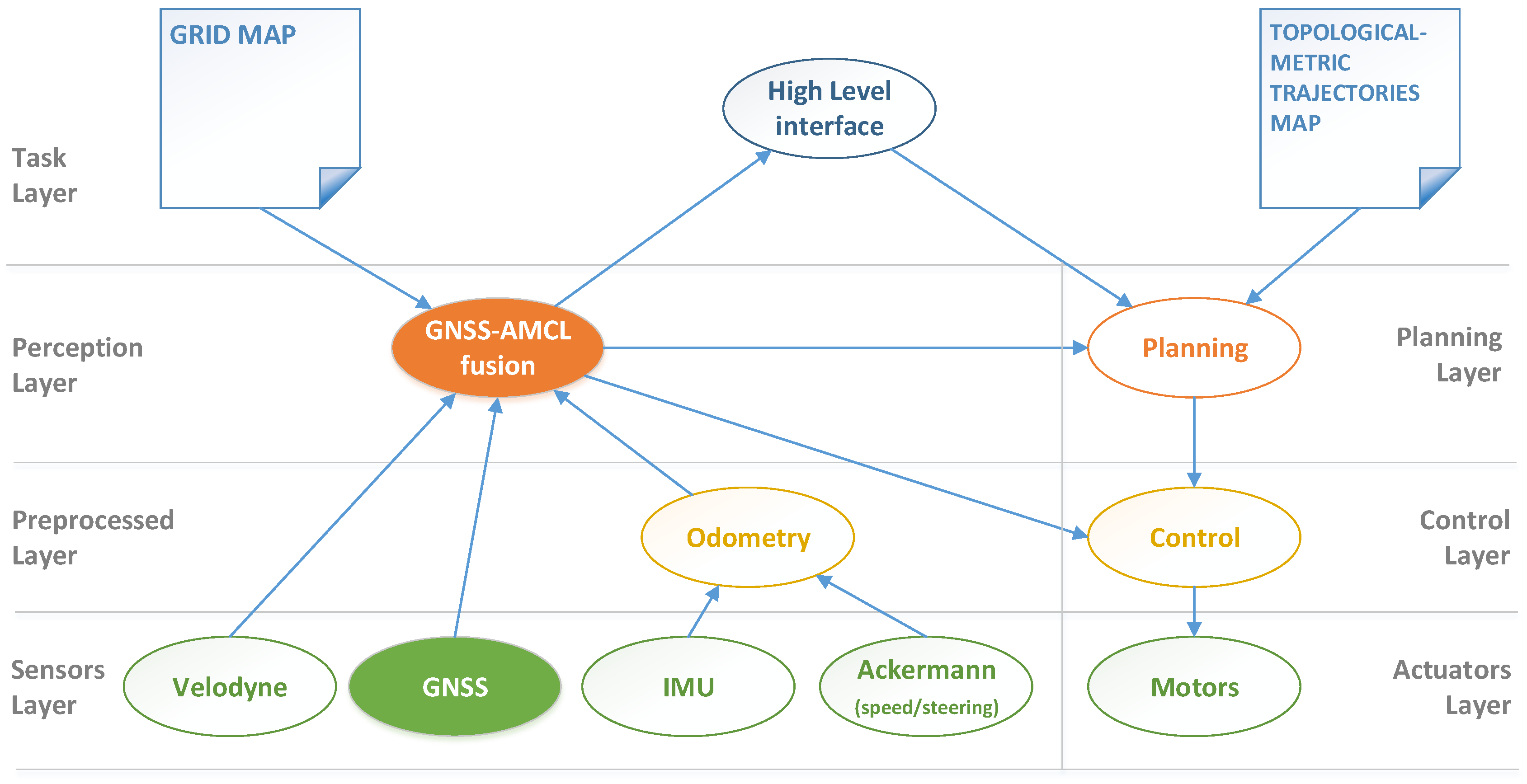
• A generic navigation framework. We propose a conceptual structure for navigation problems that permits to implement complete autonomous navigation systems in a fast and easy way (although demonstrated in a ground vehicle, these implementations can be tailored to different kind of robots, whether it be terrestrial, marine or aerial). This framework permits us to easily arrange the system complexity, enabling researchers to focus on their topics of interest while generating minimal but complete applications suitable for real-world experimental testing. This feature improves the research productivity and is a direct consequence of the proposed architecture.
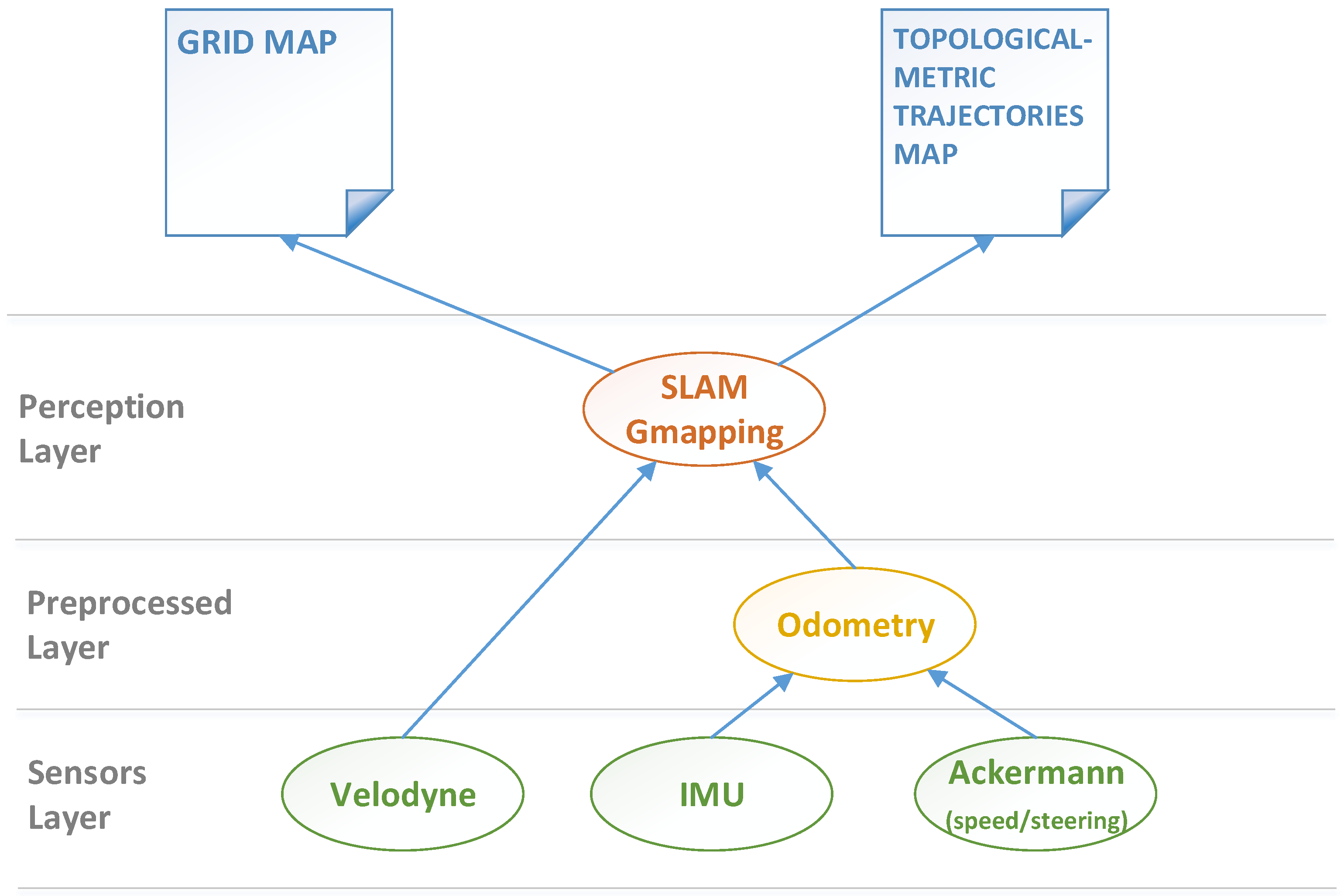
• A Kalman filter (KF)-based 2D SLAM and GNSS fusion module. To demonstrate how easy is to replace any module using the proposed framework, we developed a new localization module that became a contribution itself. This module is based on a Kalman filter that fuses the poses generated by two complementary localization sources as 2D SLAM and GNSS are. This module permits to recover the SLAM localization after exploring unmapped areas, so mixed navigation on-map/off-map can be performed.
• A set of tools for basic system implementation. In addition to the conceptual framework, we provide a set of tools that brings the basic functionalities required to implement a fully operative terrestrial autonomous navigation system. It comprises planning, car-like control, and reactive safety modules.

The rest of this paper is organized as follows: in Section 2, we describe some related works focusing on general frameworks for developing autonomous navigation systems. In Section 3, we explain the requirements and the design decisions to fulfill them, giving a conceptual architecture for our framework. Then, in Section 4, we explain the basic implementation and its features, from perception to control. Section 5 is devoted to explaining the second particularization of our framework, which implements a fusion of GNSS and Monte Carlo localization by means of a Kalman filter. In Section 6, the different experimental sessions are described and discussed, including real autonomous navigation in two different challenging outdoor environments. Finally, in Section 7, we give conclusions and future works.

2. Related Work

Due to the complexity of autonomous navigation systems, each work presenting a complete application has—in one way or another—implemented its own system architecture and navigation framework. Early examples of papers describing a complete system able to navigate outdoors in large environments are found in the eighties, like in [17,18] where Carnegie Mellon researchers developed a system to navigate autonomously through a network of sidewalks and intersections in the CMU campus. More recently, the two editions of the DARPA grand challenge [19] and the DARPA urban challenge [20] boosted the development of autonomous cars, producing a great number of contributions to the field and several papers describing the architectures and designs developed by the participant teams [11,21,22]. Observing these works, one can find that the different architectures share some features—like parallel processes, communications, tasks, etc.—which could be reusable between them, and that was one of the major reasons that motivated the creation of ROS [23]. The ROS navigation stack is the most widely spread and well-known framework to develop autonomous navigation applications. The navigation stack provides a great number of useful tools but has some limitations [24]: it is designed to operate only with differential drive and holonomic robots, it assumes that the robot can be controlled by means of a twist message indicating x, y and theta velocities, it needs a planar laser for localization and mapping and it performs best with nearly square or circular robots. There exist some workarounds like plug-ins to use it with car-like robots [25] and data conversions that can help to incorporate other sensors like the well-known Kinect depth camera [24], however the tightly coupled architecture of the navigation stack results rigid in operation [26]. In contrast, we adopt—as it will be later explained with detail—a clear architecture based on abstraction levels that makes easy to keep the system modular and scalable, so any module can be replaced without affecting the rest of the system. Looking at other recent literature, one can find some complete applications like [27,28,29], but these works aim to solve specific problems and are not designed for general purpose. Some efforts in producing more general frameworks for different levels of autonomous system development can also be found, ranging from very high-level project management and agile software development like in [30] to intermediate and low levels, like local trajectory planning and obstacle avoidance in car-like robots [31,32,33]. However, frameworks aiming to produce a fully operative “template system” to develop and test autonomous navigation algorithms are less common. In [12] a framework for fast designing and prototyping of autonomous multi-robot systems for unmanned aerial vehicles (UAV) is presented. This work shares several aspects with our approach, but it is focused exclusively on aerial multi-agent systems. A whole system architecture for autonomous surface vehicles (ASV) can be found in [34], while in [35] a generic framework is presented as an alternative to the navigation stack, but it focuses in planning and control of wheeled robots with different kinematic constraints rather than covering the whole navigation problem.

3. Framework Design

Our research group is currently working on developing localization algorithms for mobile robots. More specifically we are interested in the integration of GNSS information in graph SLAM algorithms. On the other hand, we would like to test these algorithms in the context of a complete autonomous application to study how the localization influences the system performance and to be able of conducting such experiments in the widest possible variety of environments. With this purpose, we first tried to implement an autonomous navigation system using the well-known ROS navigation stack. Nevertheless, we found that the tools provided by this stack were too much geared towards the use of two-dimensional grid maps, which makes difficult the integration of alternative localization algorithms as can be seen in [36]. For this reason, we designed an alternative framework that—among other interesting features—provides enough flexibility to integrate localization algorithms of different nature in an easy and convenient way. In advance of what will be discussed in this section, we summarize here the main advantages that our final framework design brings with respect to navigation stack:

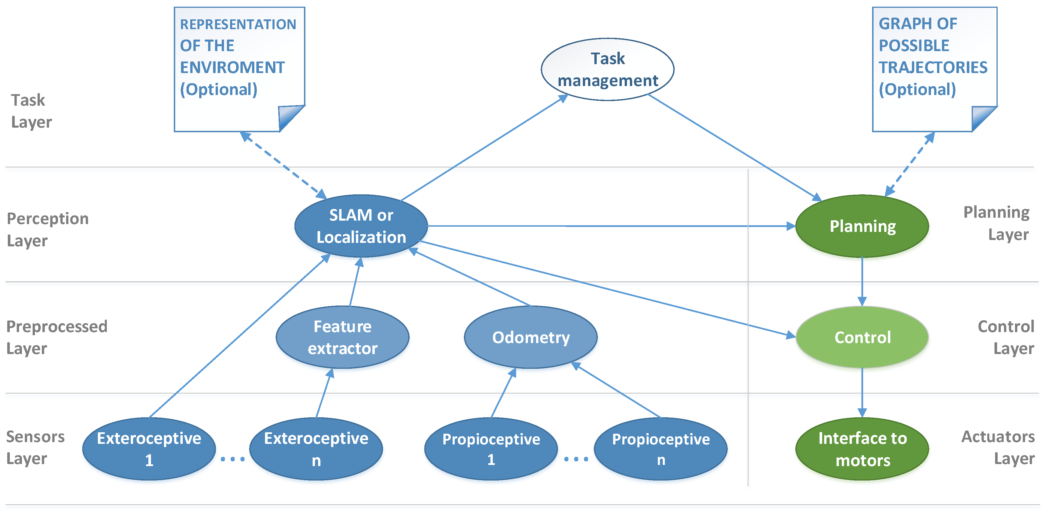
• Our planning is independent of the environment representation. In the navigation stack, global planning depends on a grid map, making it difficult to use alternative representations of the environment. On the contrary, following our approach any planning module must be independent of the environment representation, as can be seen in Figure 1. This favors modularity and eliminates conversions and other undesired extra processes required to integrate alternative environment representations with the navigation stack. An example of this can be found in [36], where the authors explain the integration of a graph-based visual SLAM system with the navigation stack planning and control modules. The authors report that they had to create a grid map from their native graph representation and that this extra process introduced additional problems that even forced to discard two of the three scenarios for the path-planning experiments carried out for the paper.
• Every ROS node belongs to a single module. The navigation stack does not follow this rule, which makes difficult the substitution of certain components. For example, the move_base node fuses planning and control, which makes it rigid in its operation [26]. In contrast, replacing modules in our framework is as easy as changing a single line in the ROS launch file. This makes the produced systems flexible and easy to adapt to different specifications (e.g., different robot kinematics, highlighted as a ROS navigation stack limitation in [24,35]) because only the related nodes need to be modified or substituted.
• Our framework follows a clear conceptual structure. In [37] we see an example of how developing a complex system using the navigation stack can lead to an intricate architecture. On the contrary, we follow a conceptual structure based on abstraction levels to make the applications clear, organized and scalable. Moreover, a neat division in conceptually different sub-problems makes easier to keep the research focus on the topics of interest without giving up the advantages that a complete system in real-world operation provides for experimental testing, as happens when using datasets or simulators.

Next, we describe the design process, starting with the requirement analysis focused on obtaining a framework flexible enough to allow fast and easy experimentation in different environments with different robots. Then, we describe the proposed design solution taking into account the specified requirements.

3.1. Framework Requirements

The key to developing a generic framework for mobile robotics is to identify precisely which parts of the software are common to different applications and design neat interfaces that permit sufficient modularity without adding unnecessary complexity to the system design. Therefore our framework requires the formalization of different software modules with standardized inputs and outputs to ease the test and comparison of different algorithms. Any algorithm change in any of its modules must be carried out in a simple way, requiring minimal changes in the rest of the system. Moreover, in order to be useful in the long term, we need to keep the framework as independent of the robot and the environment as possible.

3.2. Proposed Approach

As mentioned above, in mobile robotics applications we can distinguish different abstraction levels common to all of them. One of the requirements to develop the proposed framework is to define these abstraction levels and the software modules that are part of each one, as well as their communication channels. As shown in Figure 1, layers below task level are split in two halves to separate perception from control, resulting in three areas: perception (blue nodes), motion (green nodes) and high-level (white nodes). The links shown in the Figure 1 can be modified depending on the inputs/outputs of each particular node.

3.2.1. Perception

The lowest level we define in perception is the sensor layer. Software modules belonging to this abstraction layer are drivers to decode the information captured by the sensors. We divide the sensors into two types: exteroceptive and proprioceptive. Exteroceptive sensors are those that provide environment perception, while proprioceptive ones are those that give the information to generate the odometry. In the next perception level, we define the preprocessing layer in which we place the necessary modules to extract the information from the different sensors, implementing data fusion algorithms if required. Then, we define the highest abstraction level in the perception area to place the localization or SLAM module. Depending on the localization system we are using, the output pose of this module can be expressed with respect to different frames (local, tracked object, map or global coordinates). This localization module is designed to receive their inputs in a ROS standard format making transparent the lower layers, so there is no difference if the data comes from the sensor layer or preprocessing one. In this level, there might also be modules for scene understanding or to detect obstacles and moving objects.

3.2.2. Motion

At the highest level of motion, we define the planning layer. In this level we can integrate different software modules, that will be selected depending on the task we want to perform. Some task examples could be reaching a global goal within an environment or following a moving target, such as a vehicle or a pedestrian. For these two examples, we would need two different planners. Planner selection comes from the high-level area of the system. We also receive the robot location from the perception layer and the information obtained through the scene understanding. The intermediate level in motion is the local control. Controllers integrated into this level receive local goals from the upper layer, as well as the robot pose. The lower layer in the motion area is the actuators layer, where the software modules are drivers for communication with the robot motors.

3.2.3. High Level

At the highest level, we define the task management module. A task gets completely defined by a specific combination of modules. Therefore the task manager is in charge of deciding which modules of the lower layers will be executed. This module can also serve as a high-level interface with the agent (the user) or other robots, allowing to develop collaborative robotics applications, which is a relevant topic [38]. This last feature covers one of the limitations of the navigation stack described in [26].

4. Initial Framework Implementation

In this section we describe the basic implementation of the proposed architecture using the abstraction levels described above (Figure 2 and Figure 3). We can use this basic structure of nodes and topics as a starting point to create more sophisticated applications easily and quickly, simply by replacing the desired modules. The creation of a real-world autonomous navigation application using our framework consists of two phases: pre-execution and execution. In the first one, we gather the data to generate the environment information that we will need during the execution phase.

Of course, an equivalent system could have been generated using just the navigation stack since in this first example we based the localization in a grid map. But our framework adds conceptual structuring and better modularity. That is to say, in this implementation the only module depending on the grid map is the localization. Therefore replacing this module would not affect the rest of the system (as can be seen in Section 5) contrary to what happens with the navigation stack where the planning needs a grid map to generate trajectories.

4.1. Pre-Execution Phase

In Figure 2 we show the pre-execution phase where we generate a grid map of the area in which we want to run the application. Using the localization estimated through the SLAM node we can save the trajectories traveled by the vehicle in order to reproduce them during the execution phase. In this case, we use a GMapping node [39] but it could be replaced by any other SLAM algorithm—if we want to have an environment representation—or even by any localization algorithm (including GNSS) if we do not need a map.

4.2. Execution Phase

Figure 3 shows the architecture proposed as a closed-loop application for testing software modules in autonomous navigation. In the left part of the diagram, we show the different abstraction levels in perception, from the sensor layer to the localization module. This localization module could be replaced for any another, either SLAM-based or GNSS-based. This feature is useful to compare, in the same environment, the localization algorithms under development with well-known state-of-the-art algorithms. In the basic configuration, our localization module consists of a Monte Carlo localization (AMCL) algorithm. On the right side of the diagram, we show the different abstraction levels in the action domain, from high-level planning to the actuators layer. This is the closed-loop part where we can observe how localization affects planning and control. In the upper part of the scheme, we show a node that will serve as a high-level interface with the external agent. Using this interface we can visualize the position of the robot in the map and we can act on the system by sending global goals.

Below we describe the most important modules of our application in perception and motion. We also dedicate the last subsection to describe the reactive safety system implemented to avoid collisions.

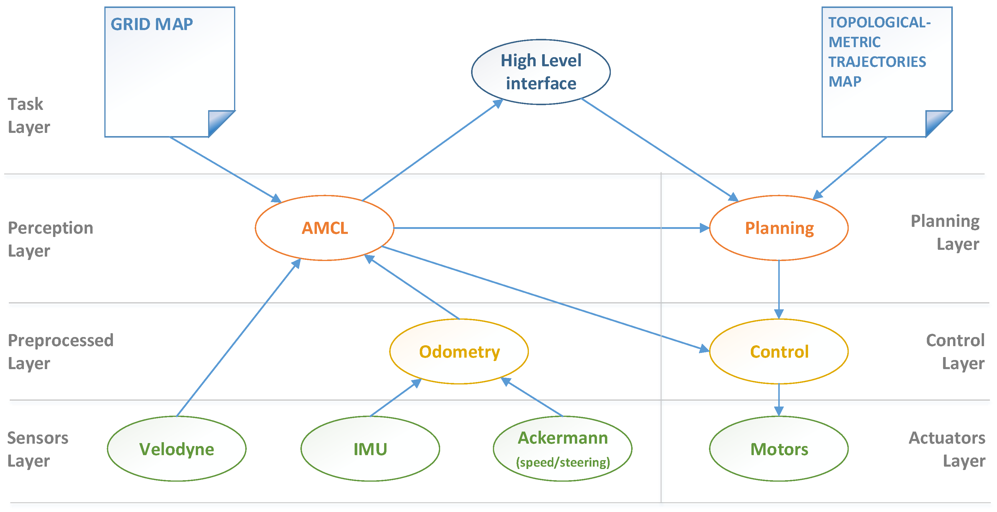
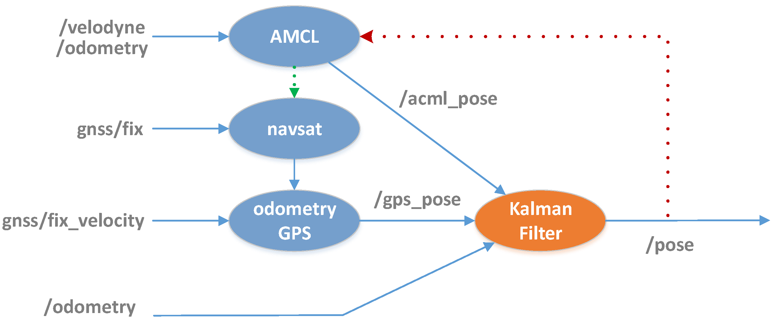
4.2.1. Localization Module: AMCL

In the basic configuration of our system, once we have a grid map obtained using GMapping (Figure 2), we need an algorithm to locate the robot inside it. We rely on the well-known AMCL. This algorithm is based on the method described in [40] and is part of the ROS navigation stack [24]. AMCL is based on the Monte Carlo approximation applied sequentially, which in the literature is called a particle filter. This method uses the sensor model described in the section beam models of range finders in [40]. It also uses the action model described in the odometry motion model section in [40]. In order to adjust the AMCL parameters, we must follow the processes described in the given references. In Section 6.2 we show the parameters obtained through these processes. This module accepts as inputs the odometry of the robot, and laser scans from a light detection and ranging (LiDAR) sensor, in our case a Velodyne VLP-16. These inputs are standard ROS messages, which eases the process of using different LiDAR sensors or even robots with different odometers. The output of this module is also a standard ROS pose message containing pose and covariance information. These covariances will play an important role in the new localization module described in Section 5, where the AMCL estimation will be fused with GNSS information by using a Kalman filter. Thanks to this structure of inputs and outputs we can replace this localization node without affecting the rest of the architecture.

4.2.2. Planning

At the top level of the motion part of the system, we defined the planning module. At first, we assessed the possibility of implementing the planner available in the navigation stack of ROS. Finally, we discarded this possibility due to the lack of versatility of this system in terms of the localization algorithms that can be used, since the planners of this stack are based solely on grid maps to obtain the trajectories. The interest of our research group is focused on the localization of robots, and we plan to use other ways to represent the environment apart from grid maps, or even transit through unmapped areas (Section 5). For this reason, we decided to develop our own system: a simple and functional planner that is more easily adaptable to any localization algorithm.

For the developed planning module, we use a topological-metric map that contains all the possible trajectories required by the target application that we want to generate using our framework. This trajectory map is generated in the pre-execution phase as shown in Figure 2. We represent these trajectories by means of a graph in which each node represents an intersection, and each link represents the path between the intersections. Each node contains information of its location in map coordinates, and each link contains equidistant points also expressed in map coordinates. This metric information is obtained in pre-execution by recording the trajectories during manual driving, next sub-sampling them, and finally assigning each point to the node or link to which it belongs. In Figure 4 we can see an example of a graph that expresses in a topological way all the possible trajectories for a certain environment and application. The inputs to this module are the graph described above, the position obtained through AMCL (or an alternative localization module), and the global goal received from the high-level interface. With this data, the module generates as output the combination of nodes and links that describes the shortest path to the global goal within the graph. This path is composed of the points expressed in map coordinates that are sent sequentially to the low-level control as local goals. This planner assures that the robot circulates always through traversable areas.

4.2.3. Control

At the level below the planning, we find the local control level of the vehicle. In this case, we also developed a basic and functional controller designed for low-speed vehicles—in the case of our robot roughly 1.3 m/s of maximum speed. The developed controller is designed for Ackermann vehicles, but given the versatility of the framework, it would be easy to integrate a new controller for vehicles with different kinematic constraints.

The aim of local control is to reach a local goal. Once it is reached, this module warns the upper level (planning) requesting a new local goal. The controller tracks the straight line that joins two consecutive goals (Figure 5, left). These lines can be generated with only one point since the orientation is specified in the ROS pose message used to communicate the goals. The controller is proportional to the error signals in distance and angle with respect to the line. Error signal in distance $e_d$ is obtained as the distance between the vehicle base link and the nearest point in the goal straight line (green in Figure 5, right). Error signal in angle $e_{\alpha }$ is obtained as the angle between the goal line (green in Figure 5, right) and the orientation vehicle line (red in Figure 5, right). The control action consists of two variables: steering angle (u), and speed (v). On the one hand, we compute the desired steering angle u as (Figure 6):

$$u=e_d{k}_d+e_{\alpha }{k}_{\alpha },$$

(1)

where $e_d$ and $e_{\alpha }$ are the errors in distance and orientation respectively, and where $k_d$ and $k_{\alpha }$ are constants adjusted experimentally for each vehicle in which the framework is implemented. On the other hand, the $e_d$ error is saturated so that $\left|u\right|$ does not exceed the maximum possible value $u_{max}$. This saturation is required because the linear speed applied as a part of a control action is calculated as a function of the steering as:

$$v=v_{max}-\left|u\right|k_v,$$

(2)

where $k_v=v_{max}-v_{min}/u_{max}$, $v_{max}$, and $v_{min}$, are the maximum and minimum velocities configurable as parameters. Note that if $\left|u\right|>u_{max}$, the resulting speed would be less than $v_{min}$. For this reason we saturated the $e_d$ error signal shown in (1). Figure 6 shows the block diagram of the described controller for steering variable.

4.2.4. Safety

Between the levels of sensors and preprocessing in perception, and between the levels of control and actuators in motion, we implement a reactive hidden layer for safety reasons. In the perception part, we designed a module that given the LiDAR point-clouds and the steering angle returns the distance to the closest point of the closest reachable obstacle. Based on this distance and a safety margin, we calculate the maximum safe speed that is defined as the one required to reach the minimum distance allowed to the obstacle in a safety period of seconds (user configurable). As the vehicle gets progressively closer to the object the speed is reduced due to the fact that the safety period is constant. Finally, when the minimum distance is reached the safety speed is just zero. In the motion part, we implement a speed recommender that reads the speed contained in the control action and the maximum speed calculated by the obstacle detector sending the lowest of them to the actuators. Thus, if the vehicle finds an obstacle along its trajectory it will stop at a defined safety distance and it will wait until the obstacle gets away from the robot. If there are no close obstacles the vehicle will recover its original speed.

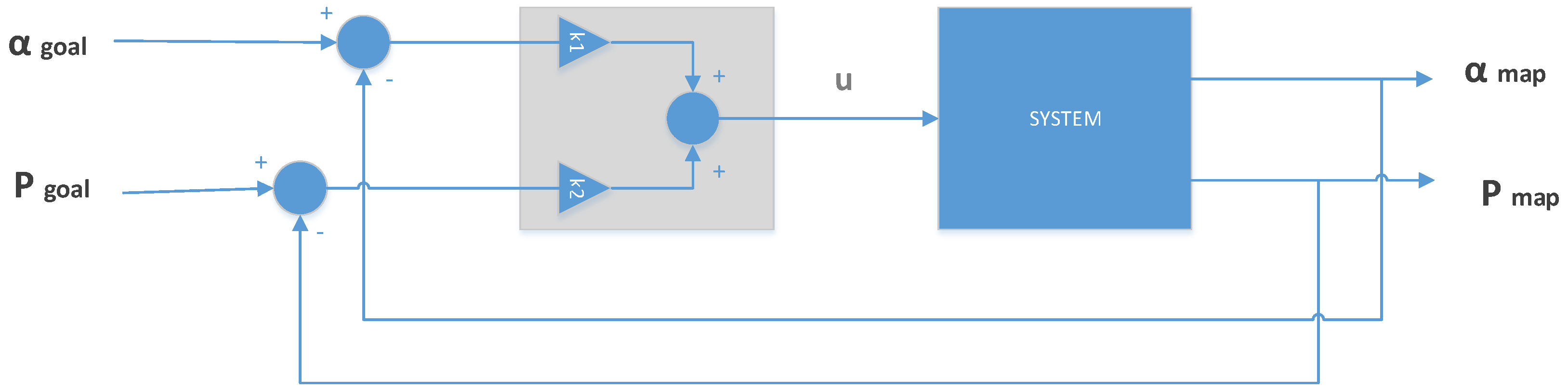
5. New Localization Module: GNSS/SLAM Fusion

One of the research lines that our group wants to develop in the future is the fusion of SLAM algorithms with GNSS-based systems. The motivation for this fusion is the complementarity of both localization systems since SLAM algorithms need relatively close landmarks to extract positional information—which can cause occlusions and multi-path problems to GNSS positioning—while GNSS systems work better in clear areas that are challenging for SLAM algorithms because of landmark scarcity. As a starting point for our future research and in order to demonstrate the versatility of our framework, we developed a new localization system based on GNSS/SLAM fusion. Figure 7 shows the ROS nodes scheme of our new localization module, and Figure 8 details its connection with the rest of the system. In our solution, we fuse the positions obtained by the two systems using a Kalman filter in which these positions will be considered asynchronous observations and the odometry is used as a control signal in the prediction phase of the filter. This module allows off-map localization, so it would be difficult to integrate it with the navigation stack but its integration is straightforward using our framework. We next describe each subsystem shown in Figure 7.

5.1. AMCL Subsystem

One of these subsystems is AMCL described in the previous section. To properly implement the fusion, we need to pay attention to the variances that this subsystem provides, associated to each estimated pose (Section 4.2.1) because they provide information about the confidence of the solution. This information will be used by the Kalman filter in the correction step, and it also will be useful for the integrity monitoring system.

5.2. GNSS Subsystem

The GNSS system provides geolocalization in world coordinates (world frame) but to perform the fusion with the subsystem described above we need to convert the global coordinates to map coordinates. For this we use the navsat node available in the ROS robot localization package [41]. In the initialization step, this node receives a position expressed in the frame we want to use as reference—in our case the position calculated through AMCL depicted as a green dotted line in Figure 7—and generates a T transformation between the pose in world frame to the map frame. Then T is applied to all the measurements made by the GNSS. By using only the navsat node, we could only read the GNSS fix and generate a 2D position in the map frame, but without orientation. To overcome this issue we generated a new ROS node called odometry GPS (Figure 7) in which we receive the velocity fix provided by the GNSS and the position and the T calculated by navsat. The output of this node is the orientation in the map frame, obtained using the velocity vector (provided by GNSS velocity fix) and the transform between the global frame and the map frame given by the navsat node.

5.3. Odometry

In a previous work [42], we described a generic module for low-level control of Ackermann type vehicles, called control logic for easy Ackermann robotization (CLEAR). From this low-level module, we obtain the linear speed and steering angle of the vehicle. For this first implementation of the framework, we developed a module to extract the positions and orientations by fusing the information obtained through CLEAR and an inertial measurement unit (IMU). This module provides as output the standard ROS message for odometry.

5.4. Kalman Filter

As mentioned above, we decided to use a Kalman filter for the fusion of the two high-level localization subsystems. This choice is motivated by the fact that we have found a simple linear model with Gaussian noise that is sufficient to represent our fusion problem, and the Kalman filter is the optimal solution under these assumptions. It should be noted that the aim of this filter is not the localization itself, but to fuse sources from complex localization algorithms that provide filtered information. For this reason, we can simplify the model and avoid the Extended Kalman filter and its problems derived from linearization. The state vector in this model is a pose vector: $\mathbf{x}={\left(xy\theta \right)}^T$. The state transition equations $\mathbf{x}\leftarrow f({\mathbf{x}}_{k-1},\mathbf{u},\mathbf{w})$ are defined as:

$$x_k=x_{k-1}+\Delta u_x+w_x$$

(3)

$$y_k=y_{k-1}+\Delta u_y+w_y$$

(4)

$${\theta }_k={\theta }_{k-1}+\Delta u_{\theta }+w_{\theta },$$

(5)

where $\mathbf{u}={\left(u_x{u}_y{u}_{\theta }\right)}^T$ is the control signal, which in this case is the odometry generated by our low-level system, being $\Delta \mathbf{u}={\mathbf{u}}_k-{\mathbf{u}}_{k-1}={(\Delta u_x\Delta u_y\Delta u_{\theta })}^T$, where $\mathbf{w}={\left(w_x{w}_y{w}_{\theta }\right)}^T$ is the system perturbation noise. As the state is fully observable by the two subsystems described, the observation equation is defined as:

$$\mathbf{y}=H{\mathbf{x}}_k+v,$$

(6)

where $\mathbf{y}={\left(y_x{y}_y{y}_{\theta }\right)}^T$ is the observation vector from the localization subsystems, and where $\mathbf{v}={\left(v_x{v}_y{v}_{\theta }\right)}^T$ is the observations noise. As the observations are of the same nature as the state vector, the matrix that relates them is an identity matrix $H=I_{3x3}$. Using this Kalman filter implementation, we can obtain a high-frequency prediction step which rate is given by the odometry (see (3)–(5)), while applying the filter correction step only when a new high-level observation becomes available. In this way, the positioning rate is sufficient for the control loop. We follow the notation used in [40] where a thorough explanation of Kalman filter equations can be found.

5.5. Integrity Monitoring

The entire information flow between the localization subsystems and the Kalman filter passes through an integrity monitoring module to avoid possible undesired behaviors. Each time an observation is generated from any high-level subsystem, we compute the Mahalanobis distance between the prediction and the observation to reject outliers. The rejected observations are excluded from the Kalman filter correction step.

The integrity monitoring module also permits to correct the AMCL subsystem using the Kalman filter output, as we can see in Figure 7. This recovery procedure is especially useful to leave and return from/to the mapped area. The monitoring module will allow this correction step in cases where the AMCL variances exceed a certain threshold. To ensure the localization stability, this correction is applied only to the state vector of the AMCL, leaving the covariances as they are. This procedure helps to the convergence of the system when re-entering to a previously mapped area.

6. Experiments

In this section, we give a brief description of the robotic research platform used for the experimental sessions (Figure 9) and a thorough explanation of the experiments performed to test both the autonomous navigation application proposed in Section 4 and the localization module proposed in Section 5. In addition, we justify the choice of the adjustable parameters of the system.

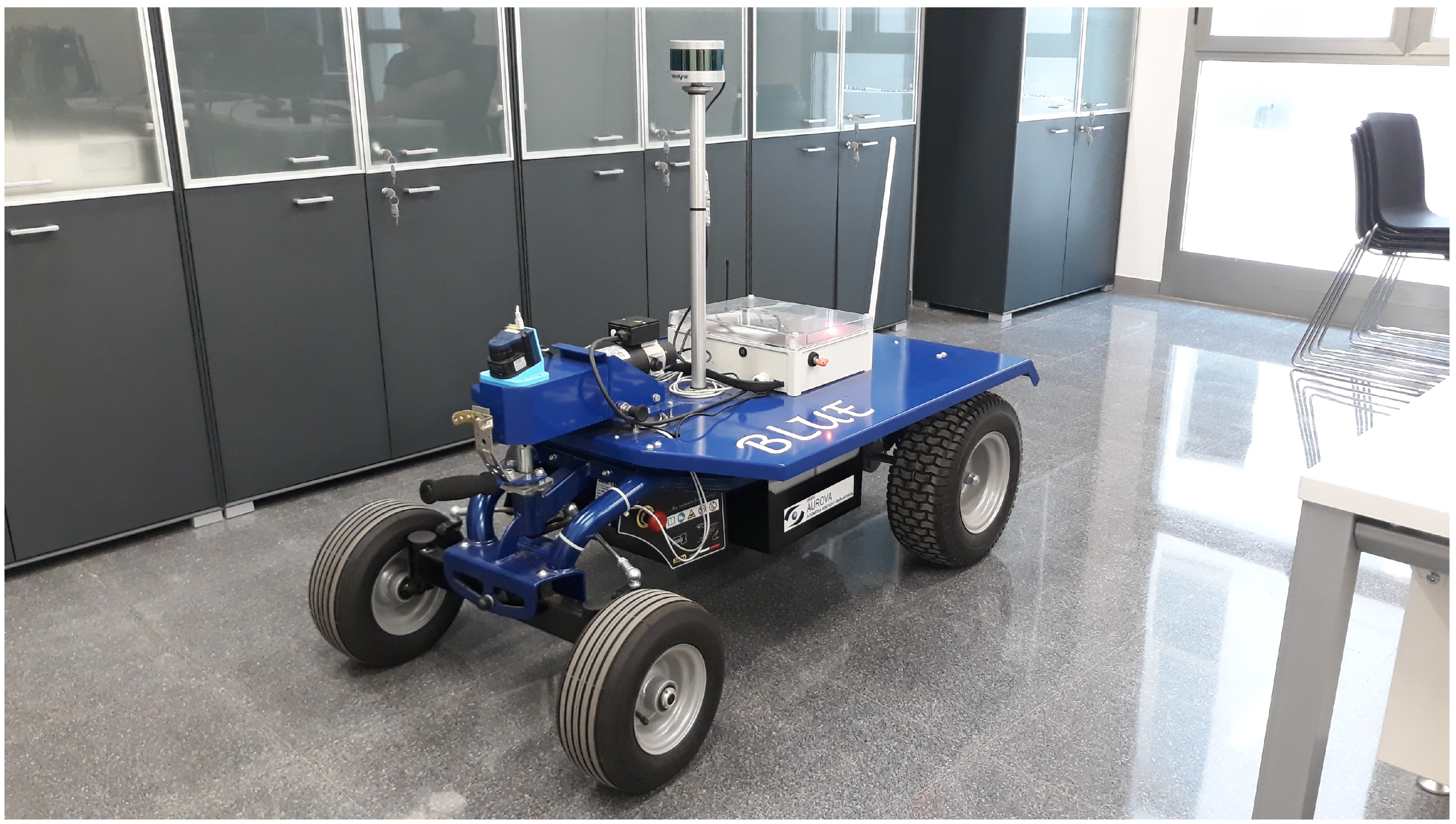
6.1. Experimental Platform

To carry out the experimental part of this work, we implemented the solution described in Section 4 using the robotic research platform BLUE. This robot is derived from a conventional electric cart and has been developed entirely by our research group, AUROVA. It has been designed to ease the experimental processes in mobile robotics research [42] and incorporates a powerful low-level module—also developed by our group—that is called control logic for easy Ackermann robotization (CLEAR). This module permits to turn conventional Ackermann vehicles into research robots integrated into ROS [42], and provides—besides other interesting features—a very accurate estimation of the steering angle and the platform speed even using extremely-low resolution sensors [43]. The robot main hardware components are the following: 3D LiDAR sensor Velodyne VPL16, 2D LiDAR sensor Hokuyo UBG-04LX-F01, RGBD camera Intel Realsense D435, GNSS real-time kinematic (RTK) capable Ublox M8P, and IMU sensor CHR-UM7, among others. It also has an onboard computer in which sensors and actuators are integrated via ROS. This computer is also used to run the system implemented following the architecture shown in Figure 2 and Figure 3.

6.2. Settings

In Section 4 and Section 5, we commented about different configurable parameters, some that depend on the robot used to implement the application, and others depending on the selected environment. In

Table 1. Adjustable parameters grouped in subsystems. The table shows the values used in the experimental sessions. Some parameters depend on the robot, as is the case with the parameters $\alpha$ of AMCL, while others depend on the environment, as the map resolution in GMapping.

Module	Parameter	Value	Units
GMapping	Grid resolution	0.05	m
	Maximum map dimensions	100 × 100	m
	Number of particles	30	none
AMCL	${\alpha }_1$	1.12	none
	${\alpha }_2$	0.1	none
	${\alpha }_3$	1.05	none
	${\alpha }_4$	0.1	none
Planning	Subsampling distance	2.0	m
Control	Constant $k_d$	8.0	none
	Constant $k_{\alpha }$	0.5	none
	Maximum speed	1.0	m/s
	Minimum speed	0.6	m/s
	Maximun steering	25.0	deg
Kalman filter	Noise model for $xy$ components	0.05	m
	Noise model for $\theta$ component	0.58	deg
Integrity monitoring	Mahalanobis distance threshold	3.0	none
	AMCL correction threshold for $xy$ components	3.0	m
	AMCL correction threshold for $\theta$ component	10	deg

we specify the parameters used for the experimental sessions described in this section. In [44], we can see the large number of default parameters that GMapping uses. We choose to limit the experimental tunning process to just the three parameters shown in Table 1. However, our tunning process ended up replicating the default values, so our GMapping configuration is the same as the standard one. In the case of AMCL we obtained the $\alpha$ parameters from the motion model as described in [40], leaving the rest of default AMCL parameters [45] unchanged. The planning module has only one adjustable parameter, which is the distance between local goals (Section 4.2.2). For the control subsystem, we show the value of the control adjustment constants described in (1) which are obtained empirically, as well as the maximum and minimum speeds and the maximum steering angle, that were selected by design, taking into account the physical limitations of the robot. For the Kalman filter based fusion system, we adjusted the model noise variances empirically and used the variances provided by the AMCL and the GNSS modules as observation noises. In Section 5.5 we discussed the outlier rejection process—that depends on a Mahalanobis distance threshold—and the maximum AMCL variance threshold that activates the recovery process of the Monte Carlo estimator. The adjustment of these thresholds has been done experimentally, looking to obtain the best qualitative results.

In the rest of this section, we describe and discuss the experiments performed using the configuration described in Table 1.

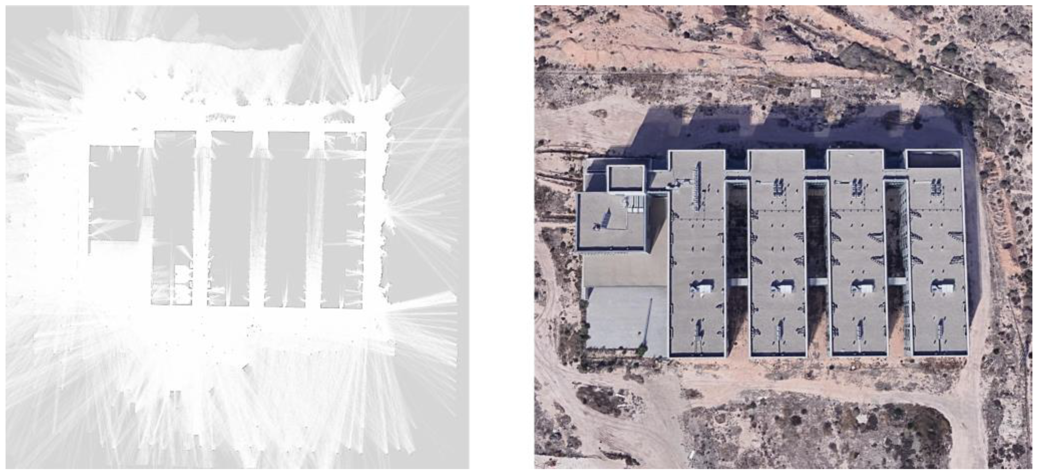
6.3. Initial Framework Experiments

To test the initial framework implementation described in Section 4, we carried out an experimental session in the surroundings of the University Institute for Computing Research building, where the secondary laboratory of our research group is located (Figure 10, right). For this experiment, we used our framework to create a basic but complete autonomous navigation application able to navigate indefinitely repeating the same trajectory in the described environment. Following the procedure detailed in Section 4, the experimental session was divided into two phases: pre-execution, and execution.

In the pre-execution phase, we recorded a dataset in manual driving making a closed loop around the building shown in Figure 10, right. Then, offline we ran this dataset in order to generate the inputs for the architecture shown in Figure 2. As result of this process we obtained a grid map (shown in Figure 10, left) and a subsampled trajectory as described in Section 4.2.2. Thanks to the use of standard ROS launch files we can run the whole pre-execution system with just one click. In the online execution phase, we used the architecture shown in Figure 3 to replicate autonomously the trajectory obtained in the previous phase, cyclically and indefinitely.

The use of a roslaunch file made the starting process fast and easy. During the experiment, the system behavior was quite good. The localization was very stable, allowing the robot to complete the experiment—consisting in five consecutive laps around the building—without interruption. The system demonstrated a good repetitiveness with very small variations in the trajectories from lap to lap. The control was smooth and stable along the entire path adapting perfectly to the given trajectories without suffering any oscillations. This first experiment proved that our framework is able to produce a real autonomous navigation application quickly and easily, requiring just the execution of two launch files. As we can see in [24], it would be also possible to perform an equivalent experiment using the tools provided by the navigation stack and some plug-ins. However, in the following section, we demonstrate the versatility of our framework by changing the localization system to navigate on and off-map, which would have not been possible using the navigation stack.

6.4. GNSS/SLAM Fusion Framework Experiments

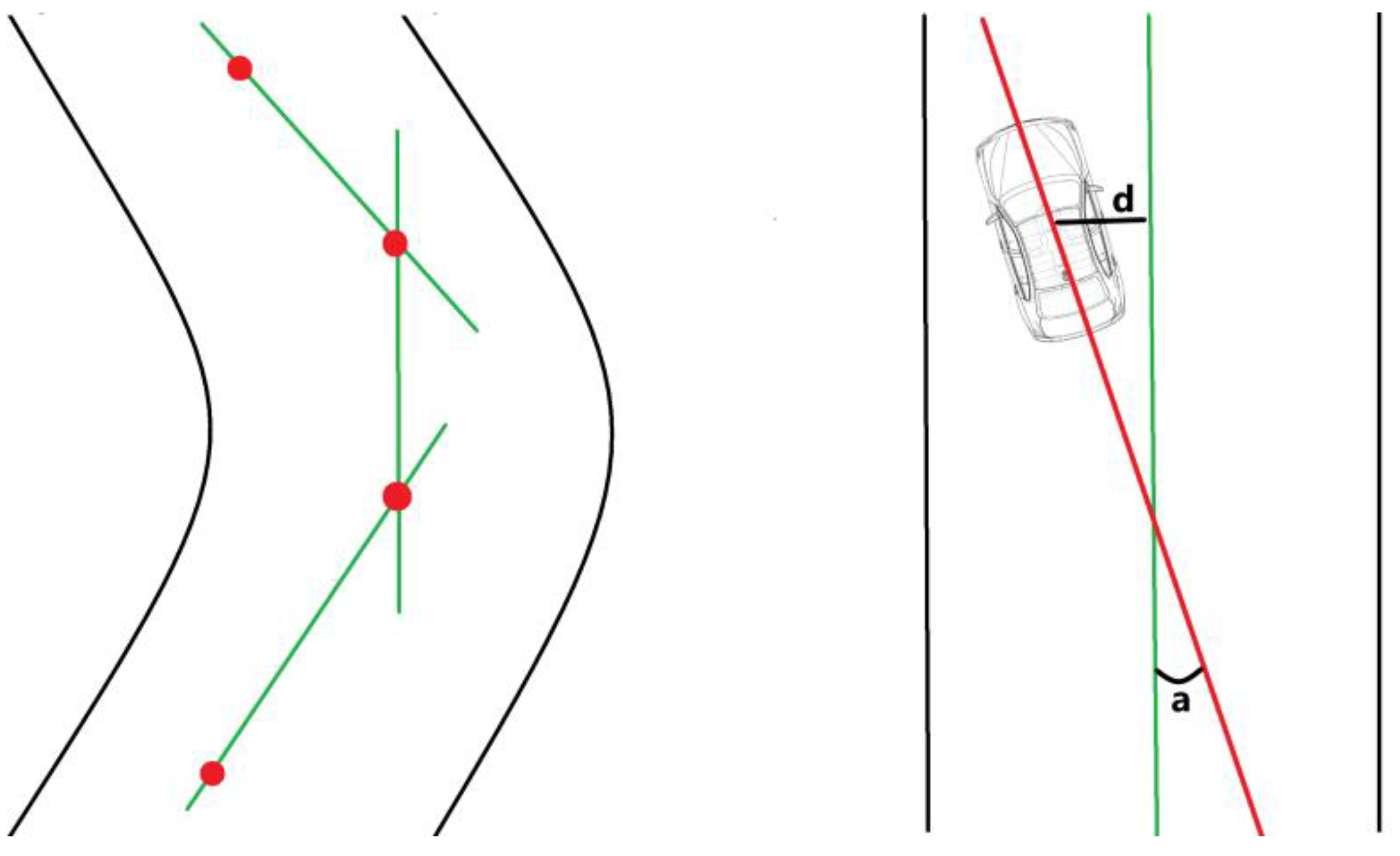
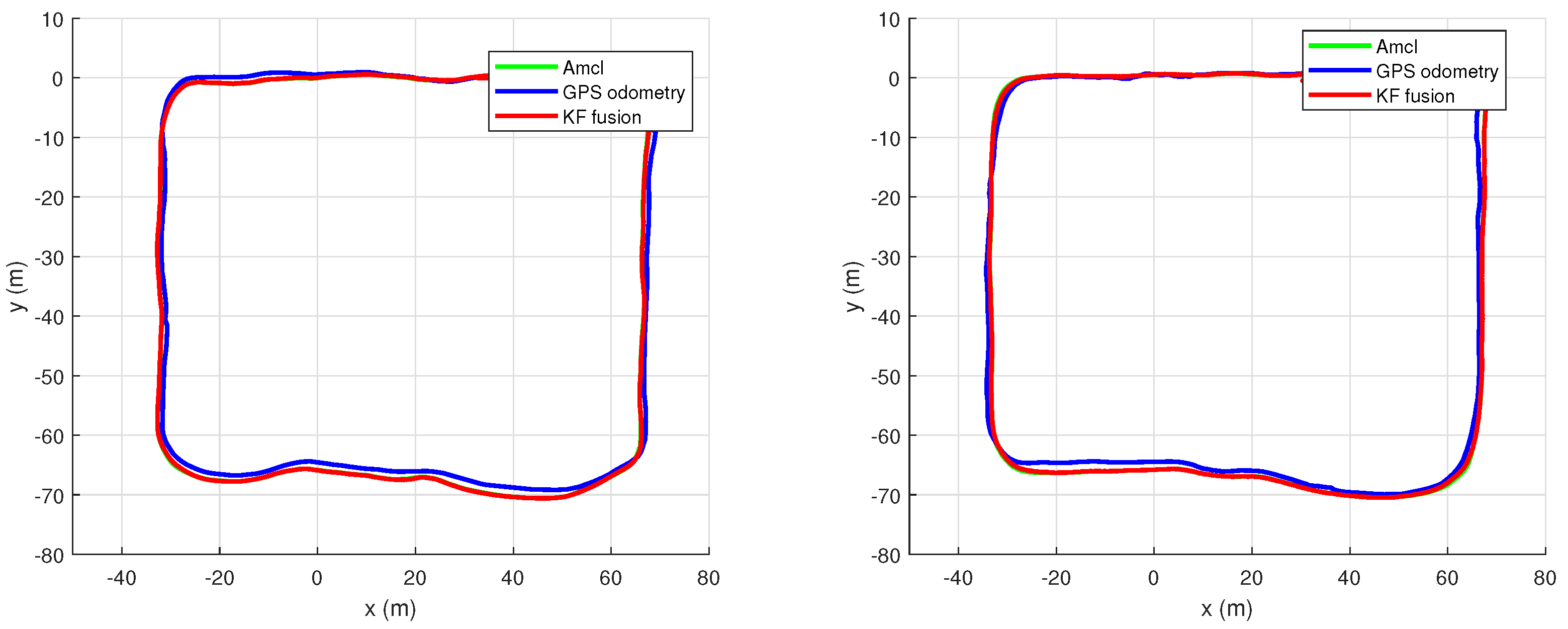
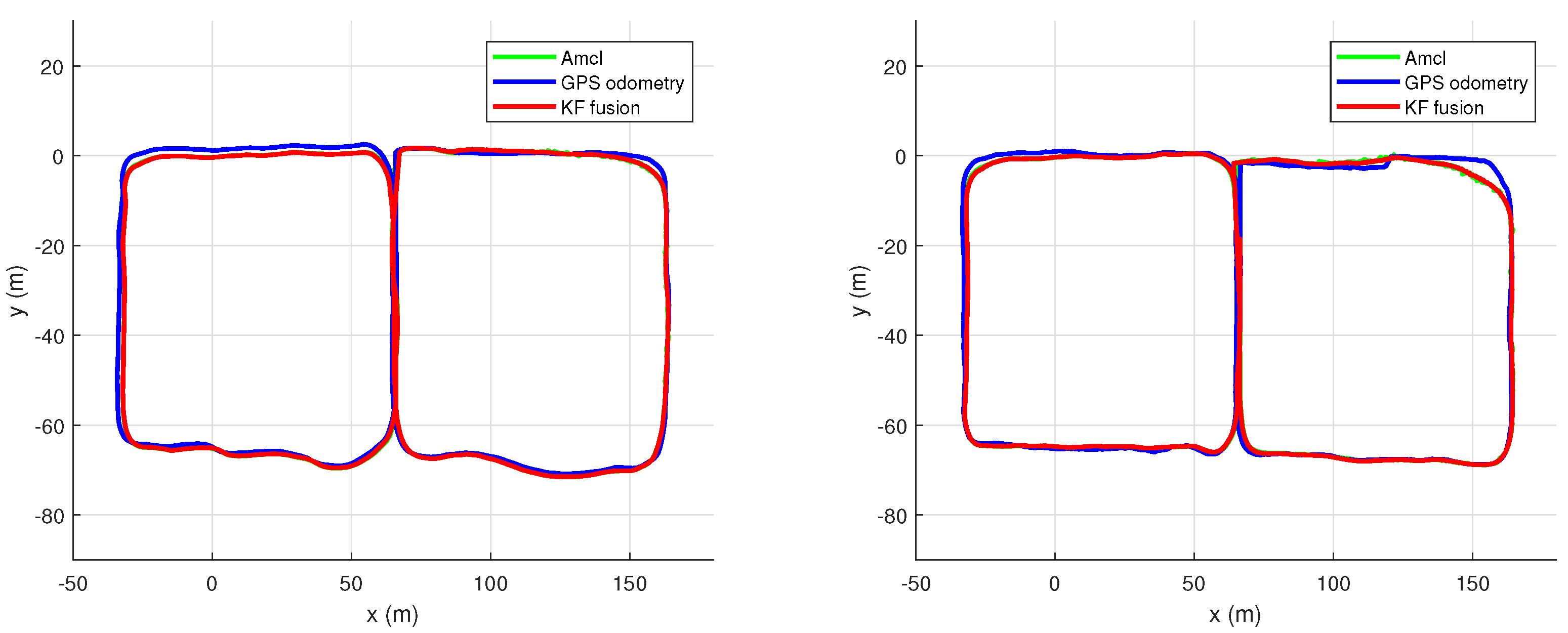
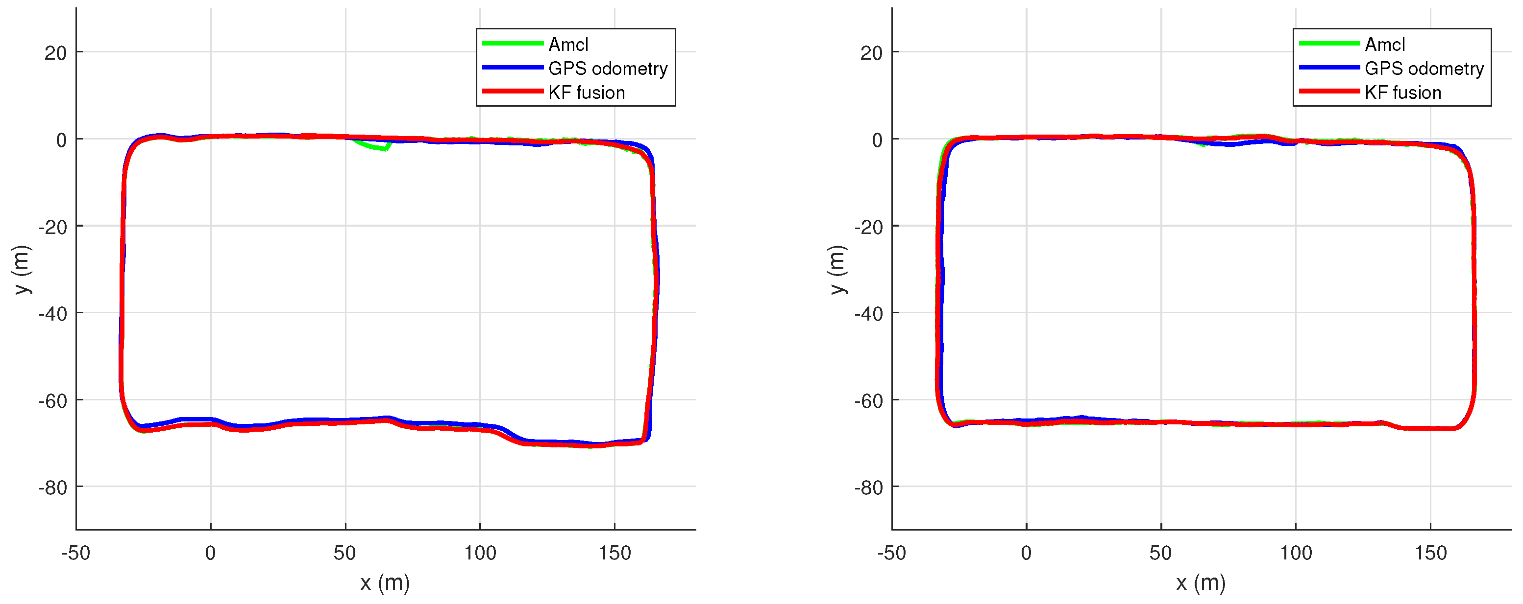
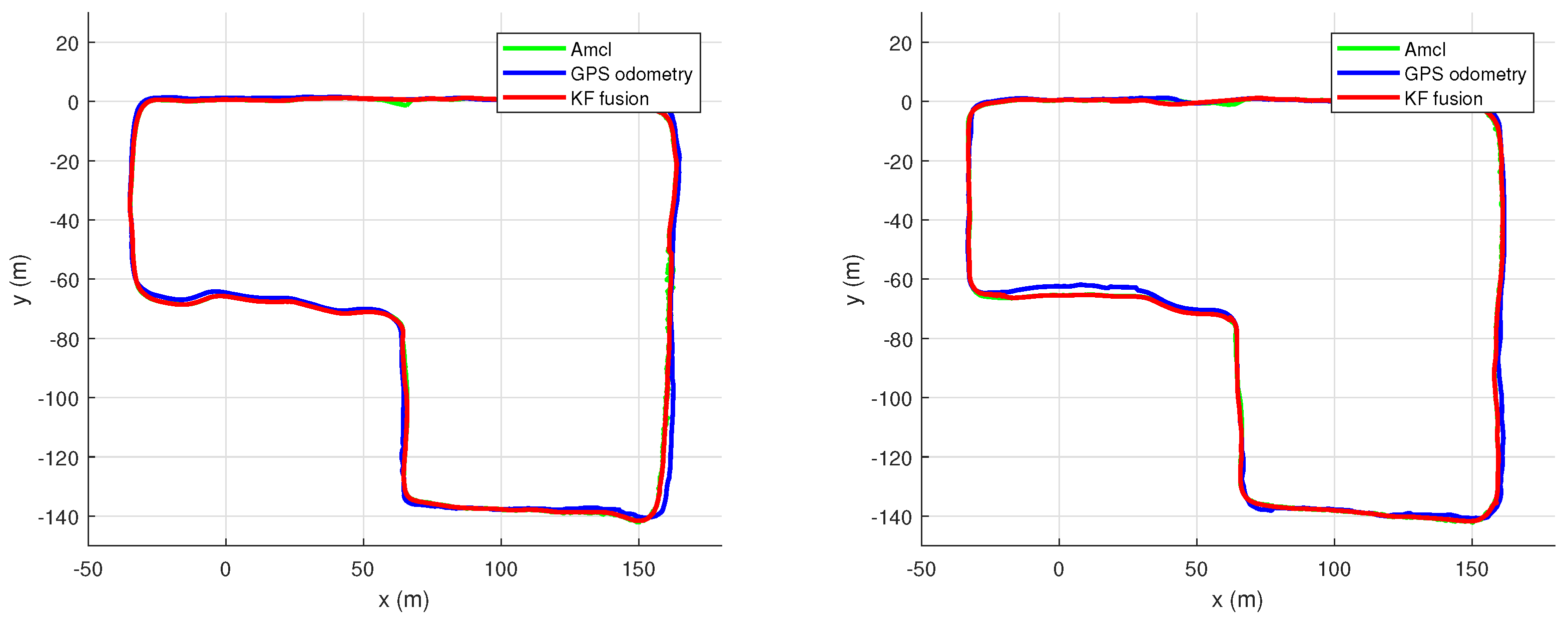
To demonstrate our framework versatility, we generated a second application in a different environment. In this case, we replaced the original localization module with the fusion module described in Section 5. Our framework permitted to make this replacement by just changing the corresponding extensible markup language (XML) tag in the launch file of the execution phase without worrying about other nodes and component interactions. The rest of the process to create the application was exactly the same as the one described in the previous section. In this way, we verified the easiness that our framework provides to test new algorithms within a fully operative autonomous navigation application. Concretely, in this case, it would have been very complicated to generate an equivalent application using the navigation stack since it was not prepared for off-map navigation.

In the rest of this section, we describe and comment on the experiments carried out to test the second application generated using our framework. We tested the new localization module observing how it affected the whole autonomous navigation system. We performed these experiments on the University of Alicante campus (in the area whose grid map is shown in Figure 11) because it was an environment where we can find different scenarios that may affect the localization of our vehicle. For example, there were areas with high trees and buildings—that could cause satellite occlusions affecting the GNSS—and lots of dynamic obstacles, such as pedestrians, electric maintenance cars, or even road vehicles, that can affect the Monte Carlo localization.

6.4.1. Localization

To test our new localization module (described in Section 5) we followed different paths through the campus. These routes were recorded in manual driving using a remote control. To test the fusion of the different localization subsystems these paths pass both within a grid map, previously obtained using the architecture shown in Figure 2, and outside it. We obtained this map through the datasets recorded for the experiments of our previous work [42]. Using this map, we are able to locate our vehicle in the environment using AMCL. However, it has been six months since the data was captured. This means that in the map may appear dynamic objects that were in the environment at the time the map was made and that might not be in the environment when the AMCL runs. We can see this map in Figure 11. The paths we followed in the experiments are those shown in Figure 12 and Figure 13. In the path $R1$ (Figure 12 left) we circulated entirely within the map. In the path $R2$ (Figure 12 right) we circulated in part out of the map, in this way we tested how the system behaves when using only GNSS. In the path $R3$ (Figure 13 left) we circulated approximately the half of the route out of map. The difference with respect to the path $R2$ is that in this case we went out and entered the map describing a rectilinear trajectory, which can be more favorable to the relocation because AMCL suffers in the turns. The last route was the $R4$ (Figure 13, right), in which we circulated most of the journey off-map to test the non-divergence of the system. In this route, we found very unfavorable areas for the GNSS because of high trees and nearby buildings. All the paths were done twice, once with GNSS standalone, and another using the GNSS-RTK in floating mode (details about the single-frequency RTK system used can be found in [42]).

In Figure 14 we can see the trajectories obtained when following the path $R1$, with GNSS standalone (left), and with GNSS RTK floating (right). This is the only journey that we made entirely within the map. In these conditions, the AMCL localization proved to be very robust. This translates into very small variances what makes the KF output to be very similar to the output of the AMCL. As we can see in Figure 14, the red line (KF) is superimposed on the green line (AMCL), as both provide almost the same location. In both cases, we see that the blue line (GNSS) differs from the fusion, although to a lesser extent in the case of RTK.

Figure 15 shows the paths obtained for $R2$. In this case, the behavior in the map area is the same as shown in the previous case. However, in the area where we travel off-map ($x>75$ m) the fusion adapts to the observations provided by the GNSS-based subsystem. In this area, when the AMCL uncertainty grows exceeding the thresholds, the Kalman filter output corrects the AMCL state estimation so that when the robot re-enters to the mapped area the AMCL subsystem converges again.

Figure 16 illustrates the trajectories made for the path $R3$. In this case, we can observe a behavior similar to that of the path $R2$ where the fusion adapts to the GNSS system in the off-map area ($x>75$ m). In the case of the path made using the RTK system, we see that the low variances makes the fusion to closely follow the observations. For this reason, we see how the red line (AMCL) is superimposed to the rest of the subsystems in Figure 16 right.

Figure 17 shows the result of performing manual driving through the path $R4$. In this case, the trajectories run off the map in the whole area defined by $x>75$ m and $y<-90$ m. We see that the behavior is similar to the cases described for the paths $R2$ and $R3$ with the difference that in this case most of the journey is off-map and verifying that the re-entry can be done successfully even after a long journey without mapped references.

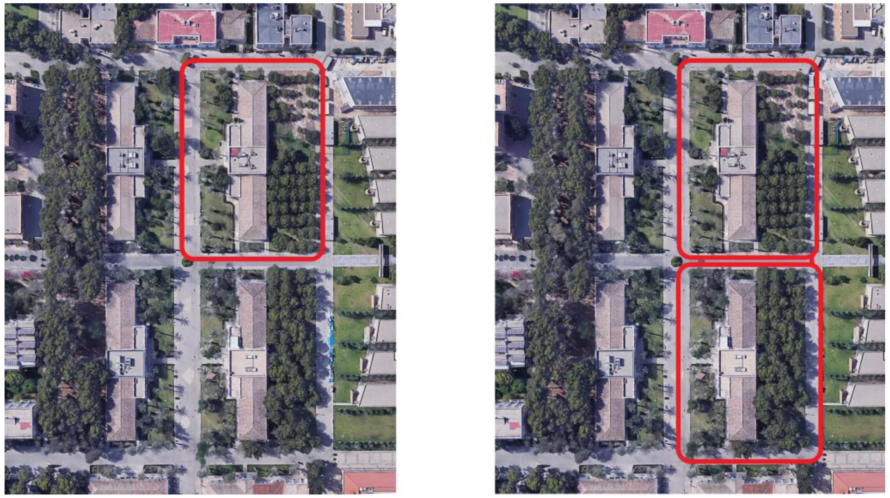
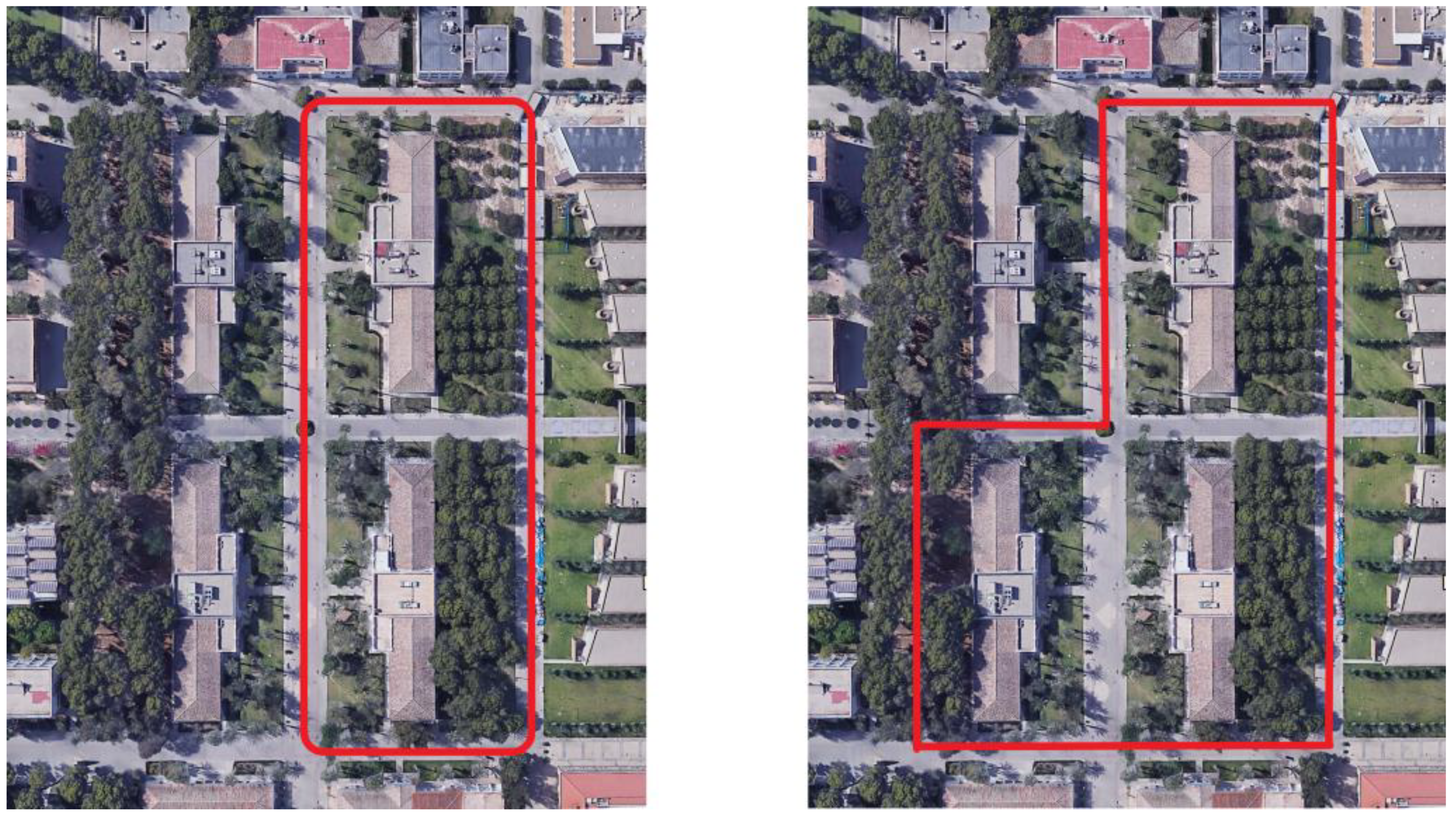
6.4.2. Autonomous Navigation

In the previous section, we described the experiments carried out to test the localization but in that case, the control loop closure was being performed by the users who handle the remote control. Because of this, we are influencing the localization by using our own human localization at the cognitive level. In order to test how location affects control, we integrated into our vehicle the architecture shown in Figure 3 to navigate autonomously in closed circuit. Using the paths recorded during the previous experiments we generated two maps of trajectories through the routes $R3$ and $R4$ (Section 6.4.1), defining two different circuits. For these experiments, the application is configured to run through the specified circuit indefinitely. In this way, we will be able to observe the repetitiveness of the trajectories in each lap. With these conditions, we carried out four different experiments. First, we performed the autonomous navigation along the circuit defined by the path $R3$ using the GNSS in standalone mode. Next, we used the circuit described by the path $R4$ also with the GNSS configured in standalone mode. In order to see how the differential corrections of GNSS can affect navigation, we repeated the two experiments previously described but using the RTK in floating mode.

The system behavior in the paths $R3$ and $R4$ with the standalone GNSS configuration was similar. In both cases, the errors of the standalone GNSS system caused failures in the zones marked with yellow circles in Figure 18. These errors resulted in emergency stops, thanks to the system described in Section 4.2.4. However, it was possible to demonstrate the system recoverability since, after skipping these areas in manual driving we were able to complete the circuit autonomously. During the RTK experiments, the system was able to complete the circuit without interruptions including the off-map areas. The behavior in these experiments was very similar to the described in the previous section: the system shown repeatability and a smooth and stable control without oscillations. However, in these experiments we were not able to circulate indefinitely, since in the second lap, in the areas marked with yellow circles in Figure 18 we lost connection with the base station, disabling the RTK mode and forcing to interrupt the autonomous navigation. As in the previous case, the system proved to be recoverable as it returned to autonomous navigation after passing these critical points.

7. Conclusions and Future Work

In this paper, we presented a framework designed for fast prototyping of autonomous navigation systems. This framework reduces dramatically the amount of work required to implement a whole application, making easier to test and to compare different algorithms in real-world conditions. The proposed architecture permits us to focus the efforts in the desired research topics, while the provided basic set of tools enables the users to generate fully operative autonomous navigation systems to perform experimental tests. To validate the described approach we used the framework and the provided tools to implement an initial basic system that was able to complete successfully several laps around a building autonomously in a challenging outdoor scenario. To demonstrate the easiness of module substitution, we developed a novel algorithm that relies in a Kalman filter to fuse 2D SLAM and GNSS positioning and used it to replace the localization module of the initial basic system. This new module was incorporated just changing a single line of the launch file. Extensive tests for this new localization module were performed navigating autonomously through mixed on-map/off-map trajectories in the University of Alicante campus. This new localization module has shown interesting properties on its own, and thus has become one of the contributions of the present work. The experimental sessions covered more than twenty kilometers in two absolutely different outdoor environments. All the software is publicly available in a GitHub repository (https://github.com/AUROVA-LAB/aurova_framework) with the aim of being a useful tool for research groups interested in any of the fields related to autonomous navigation.

As future work, we want to extend provided set of tools, adding re-planning capabilities, redundant safety modules and terrain analysis algorithms. In the localization part, we plan to integrate a graph SLAM system implementing a tight integration of GNSS raw observables and to use unsupervised learning techniques for landmark detection.

References

1. Niemueller, T.; Lakemeyer, G.; Ferrein, A. The RoboCup logistics league as a benchmark for planning in robotics. In Proceedings of the International Conference on Automated Planning and Scheduling (ICAPS)—WS on Planning and Robotics (PlanRob), Jerusalem, Israel, 7–11 June 2015; Association for the Advancement of Artificial Intelligence (AAAI): Palo Alto, CA, USA, 2015. [Google Scholar]
2. King, A. The future of agriculture. Nature 2017, 544, S21–S23. [Google Scholar] [CrossRef] [PubMed]
3. Milanés, V.; Bergasa, L.M. Introduction to the Special Issue on “New Trends towards Automatic Vehicle Control and Perception Systems”. Sensors 2013, 13, 5712–5719. [Google Scholar] [CrossRef] [PubMed]
4. Nilsson, N.J. A Mobile Automaton: An Application of Artificial Intelligence Techniques. In Proceedings of the 1st International Joint Conference on Artificial intelligence (IJCAI’69), Washington, DC, USA, 7–9 May 1969; Morgan Kaufmann Publishers Inc.: San Francisco, CA, USA, 1969; pp. 509–520. [Google Scholar]
5. Carrio, A.; Sampedro, C.; Rodriguez-Ramos, A.; Campoy, P. A review of deep learning methods and applications for unmanned aerial vehicles. J. Sens. 2017, 2017, 3296874. [Google Scholar] [CrossRef]
6. Redmon, J.; Divvala, S.; Girshick, R.; Farhadi, A. You only look once: Unified, real-time object detection. In Proceedings of the IEEE Conference on Computer Vision and Pattern Recognition, Las Vegas, NV, USA, 26 June–1 July 2016; pp. 779–788. [Google Scholar]
7. Gomes, L. When will Google’s self-driving car really be ready? It depends on where you live and what you mean by “ready” [News]. IEEE Spectr. 2016, 53, 13–14. [Google Scholar] [CrossRef]
8. Canedo-Rodríguez, A.; Alvarez-Santos, V.; Regueiro, C.V.; Iglesias, R.; Barro, S.; Presedo, J. Particle filter robot localisation through robust fusion of laser, WiFi, compass, and a network of external cameras. Inf. Fusion 2016, 27, 170–188. [Google Scholar] [CrossRef]
9. Castro-Toscano, M.J.; Rodríguez-Quiñonez, J.C.; Hernández-Balbuena, D.; Rivas-Lopez, M.; Sergiyenko, O.; Flores-Fuentes, W. Obtención de Trayectorias Empleando el Marco Strapdown INS/KF: Propuesta Metodológica. Rev. Iberoam. De Automática E Informática Ind. 2018, 15, 391–403. [Google Scholar] [CrossRef]
10. Alami, R.; Chatila, R.; Fleury, S.; Ghallab, M.; Ingrand, F. An architecture for autonomy. Int. J. Robot. Res. 1998, 17, 315–337. [Google Scholar] [CrossRef]
11. Thrun, S.; Montemerlo, M.; Dahlkamp, H.; Stavens, D.; Aron, A.; Diebel, J.; Fong, P.; Gale, J.; Halpenny, M.; Hoffmann, G.; et al. Stanley: The robot that won the DARPA Grand Challenge. J. Field Robot. 2006, 23, 661–692. [Google Scholar] [CrossRef]
12. Sanchez-Lopez, J.L.; Pestana, J.; de la Puente, P.; Campoy, P. A reliable open-source system architecture for the fast designing and prototyping of autonomous multi-uav systems: Simulation and experimentation. J. Intell. Robot. Syst. 2016, 84, 779–797. [Google Scholar] [CrossRef]
13. Siegwart, R.; Nourbakhsh, I.R.; Scaramuzza, D. Introduction to Autonomous Mobile Robots; MIT Press: Cambridge, MA, USA, 2011. [Google Scholar]
14. The Robotics Data Set Repository (Radish). Available online: http://radish.sourceforge.net (accessed on 5 May 2019).
15. Koenig, N.; Howard, A. Design and use paradigms for gazebo, an open-source multi-robot simulator. In Proceedings of the 2004 IEEE/RSJ International Conference on Intelligent Robots and Systems (IROS 2004), Sendai, Japan, 28 September–2 October 2004; IEEE: Piscataway, NJ, USA, 2004; Volume 3, pp. 2149–2154. [Google Scholar]
16. Calisi, D.; Iocchi, L.; Nardi, D. A unified benchmark framework for autonomous mobile robots and vehicles motion algorithms (MoVeMA benchmarks). In Proceedings of the Workshop on Experimental Methodology and Benchmarking in Robotics Research (RSS 2008), Zurich, Switzerland, 26–30 June 2008. [Google Scholar]
17. Kweon, I.S.; Goto, Y.; Matsuzaki, K.; Obatake, T. CMU sidewalk navigation system: A blackboard-based outdoor navigation system using sensor fusion with colored-range images. In Proceedings of the Fall Joint Computer Conference, Dallas, TX, USA, 2–6 November 1986; IEEE: Piscataway, NJ, USA, 1986. [Google Scholar]
18. Goto, Y.; Stentz, A. Mobile robot navigation: The CMU system. IEEE Expert 1987, 2, 44–54. [Google Scholar] [CrossRef]
19. Buehler, M.; Iagnemma, K.; Singh, S. The 2005 DARPA Grand Challenge: The Great Robot Race; Springer: Berlin, Germany, 2007; Volume 36. [Google Scholar]
20. Buehler, M.; Iagnemma, K.; Singh, S. The DARPA Urban Challenge: Autonomous Vehicles in City Traffic; Springer: Berlin, Germany, 2009; Volume 56. [Google Scholar]
21. Montemerlo, M.; Becker, J.; Bhat, S.; Dahlkamp, H.; Dolgov, D.; Ettinger, S.; Haehnel, D.; Hilden, T.; Hoffmann, G.; Huhnke, B.; et al. Junior: The stanford entry in the urban challenge. J. Field Robot. 2008, 25, 569–597. [Google Scholar] [CrossRef]
22. Urmson, C.; Anhalt, J.; Bagnell, D.; Baker, C.; Bittner, R.; Clark, M.; Dolan, J.; Duggins, D.; Galatali, T.; Geyer, C.; et al. Autonomous driving in urban environments: Boss and the urban challenge. J. Field Robot. 2008, 25, 425–466. [Google Scholar] [CrossRef]
23. Quigley, M.; Conley, K.; Gerkey, B.; Faust, J.; Foote, T.; Leibs, J.; Wheeler, R.; Ng, A.Y. ROS: An open-source Robot Operating System. In Proceedings of the ICRA Workshop on Open Source Software, Kobe, Japan, 17 May 2009; Volume 3, p. 5. [Google Scholar]
24. Guimarães, R.L.; de Oliveira, A.S.; Fabro, J.A.; Becker, T.; Brenner, V.A. ROS navigation: Concepts and tutorial. In Robot Operating System (ROS); Springer International Publishing: Cham, Switzerland, 2016; Volume 1, pp. 121–160. [Google Scholar]
25. Rösmann, C.; Hoffmann, F.; Bertram, T. Kinodynamic trajectory optimization and control for car-like robots. In Proceedings of the 2017 IEEE/RSJ International Conference on Intelligent Robots and Systems (IROS), Vancouver, BC, Canada, 24–28 September 2017; IEEE: Piscataway, NJ, USA, 2017; pp. 5681–5686. [Google Scholar]
26. Conner, D.C.; Willis, J. Flexible navigation: Finite state machine-based integrated navigation and control for ROS enabled robots. In Proceedings of the SoutheastCon 2017, Charlotte, NC, USA, 30 March–2 April 2017; IEEE: Piscataway, NJ, USA, 2017; pp. 1–8. [Google Scholar]
27. Brahimi, S.; Tiar, R.; Azouaoui, O.; Lakrouf, M.; Loudini, M. Car-like mobile robot navigation in unknown urban areas. In Proceedings of the 2016 IEEE 19th International Conference on Intelligent Transportation Systems (ITSC), Rio de Janeiro, Brazil, 1–4 November 2016; IEEE: Piscataway, NJ, USA, 2016; pp. 1727–1732. [Google Scholar]
28. Vivacqua, R.; Vassallo, R.; Martins, F. A low cost sensors approach for accurate vehicle localization and autonomous driving application. Sensors 2017, 17, 2359. [Google Scholar] [CrossRef] [PubMed]
29. Ferrer, G.; Zulueta, A.G.; Cotarelo, F.H.; Sanfeliu, A. Robot social-aware navigation framework to accompany people walking side-by-side. Auton. Robot. 2017, 41, 775–793. [Google Scholar] [CrossRef]
30. Dove, R.; Schindel, B.; Scrapper, C. Agile systems engineering process features collective culture, consciousness, and conscience at SSC Pacific Unmanned Systems Group. INCOSE Int. Symp. 2016, 26, 982–1001. [Google Scholar] [CrossRef]
31. Li, X.; Sun, Z.; Cao, D.; Liu, D.; He, H. Development of a new integrated local trajectory planning and tracking control framework for autonomous ground vehicles. Mech. Syst. Signal Process. 2017, 87, 118–137. [Google Scholar] [CrossRef]
32. Hernádez Juan, S.; Herrero Cotarelo, F. Autonomous Navigation Framework for a Car-Like Robot (Technical Report IRI-TR-15-07); Institut de Robòtica i Informàtica Industrial (IRI): Barcelona, Spain, 2015. [Google Scholar]
33. Rodrigues, M.; McGordon, A.; Gest, G.; Marco, J. Developing and testing of control software framework for autonomous ground vehicle. In Proceedings of the 2017 IEEE International Conference on Autonomous Robot Systems and Competitions (ICARSC), Coimbra, Portugal, 26–28 April 2017; IEEE: Piscataway, NJ, USA, 2017; pp. 4–10. [Google Scholar]
34. Stateczny, A.; Burdziakowski, P. Universal autonomous control and management system for multipurpose unmanned surface vessel. Pol. Marit. Res. 2019, 26, 30–39. [Google Scholar] [CrossRef]
35. Huskić, G.; Buck, S.; Zell, A. GeRoNa: Generic Robot Navigation. J. Intell. Robot. Syst. 2018, 1–24. [Google Scholar] [CrossRef]
36. Hartmann, J.; Klüssendorff, J.H.; Maehle, E. A unified visual graph-based approach to navigation for wheeled mobile robots. In Proceedings of the 2013 IEEE/RSJ International Conference on Intelligent Robots and Systems, Tokyo, Japan, 3–7 November 2013; IEEE: Piscataway, NJ, USA, 2013; pp. 1915–1922. [Google Scholar]
37. Guzmán, R.; Ariño, J.; Navarro, R.; Lopes, C.; Graça, J.; Reyes, M.; Barriguinha, A.; Braga, R. Autonomous hybrid GPS/reactive navigation of an unmanned ground vehicle for precision viticulture-VINBOT. In Proceedings of the 62nd German Winegrowers Conference, Stuttgart, Germany, 27–30 November 2016. [Google Scholar]
38. Romay, A.; Kohlbrecher, S.; Stumpf, A.; von Stryk, O.; Maniatopoulos, S.; Kress-Gazit, H.; Schillinger, P.; Conner, D.C. Collaborative Autonomy between High-level Behaviors and Human Operators for Remote Manipulation Tasks using Different Humanoid Robots. J. Field Robot. 2017, 34, 333–358. [Google Scholar] [CrossRef]
39. OpenSLAM: GMapping Algorithm. Available online: https://openslam-org.github.io (accessed on 5 May 2019).
40. Thrun, S.; Burgard, W.; Fox, D. Probabilistic Robotics; MIT Press: Cambridge, MA, USA, 2005. [Google Scholar]
41. Moore, T.; Stouch, D. A generalized extended kalman filter implementation for the robot operating system. In Proceedings of the 13th International Conference IAS-13 (Intelligent Autonomous Systems 13), Padova, Italy, 15–18 July 2014; Springer International Publishing: Cham, Switzerland, 2016; pp. 35–348. [Google Scholar]
42. del Pino, I.; Muñoz-Bañon, M.Á.; Cova-Rocamora, S.; Contreras, M.Á.; Candelas, F.A.; Torres, F. Deeper in BLUE. J. Intell. Robot. Syst. 2019, 1–19. [Google Scholar] [CrossRef]
43. del Pino, I.; Muñoz Bañón, M.A.; Contreras, M.Á.; Cova, S.; Candelas, F.A.; Torres, F. Speed Estimation for Control of an Unmanned Ground Vehicle Using Extremely Low Resolution Sensors. In Proceedings of the 15th International Conference on Informatics in Control, Automation and Robotics (ICINCO), Portu, Portugal, 29–31 July 2018. [Google Scholar]
44. Gmapping in ROS. Available online: http://wiki.ros.org/gmapping (accessed on 5 May 2019).
45. Amcl in ROS. Available online: http://wiki.ros.org/amcl (accessed on 5 May 2019).
Figure 1. Proposed framework design. Each node represents a software module, and each solid line represents a communication channel between modules. The dashed lines represent optional channels that might connect the localization module with a map of the environment and the planning module with a map of trajectories. The existence of these optional channels depends on the concrete localization and planning algorithms used. The different modules are organized in abstraction layers (sensors, preprocessed...) as well as in conceptual blocks denoted by colours: perception (blue nodes), motion (green nodes) and high-level (white nodes).
Applsci 09 01997 g001
Figure 2. Robot operating system (ROS) nodes scheme that shows the system architecture in the pre-execution phase for our first framework implementation. Notice that each node is placed at its corresponding abstraction level. In this phase we record data from the sensors layer and process them offline using the architecture shown to obtain the grid map and trajectories that will be used in the execution phase.
Applsci 09 01997 g002
Figure 3. ROS nodes scheme that shows the system architecture in the execution phase for our first framework implementation. Notice that each node is placed at its corresponding abstraction level. The execution is now online because it is a closed loop application that acts on the environment through the control node. For both localization and planning, we will use the files generated in the previous phase shown in Figure 2.
Applsci 09 01997 g003
Figure 4. Example of a trajectories graph expressed abstractly as a topological map. This map also includes the metric information. Each node represents the location of roads intersections, and each link contains a series of points in 2D Cartesian coordinates that will serve as local goals to the controller. This graph is obtained as shown in Figure 2, and used in execution as shown in Figure 3.
Applsci 09 01997 g004
Figure 5. (left) Representation of local goals on the road. Each local goal is expressed as a point ( x , y , θ ) . With this information, we can generate a line (in green) with an orientation θ that crosses the point ( x , y ) (in red). (right) Error signal in distance d is obtained as the distance between the vehicle base link and the nearest point in the goal straight line (green). The error signal in angle a is obtained as the angle between the goal line (green) and the orientation vehicle line (red).
Applsci 09 01997 g005
Figure 6. Block diagram that shows the proportional controller described in (1). The set-point is the position and orientation of the point closest to the line shown in Figure 5, left. The error signals are obtained depending on the position and orientation of the vehicle (Figure 5, right). Both, the set-point and the vehicle pose are expressed in map coordinates. The control signal u is the steering value expressed in degrees, that we send to the low-level control module of our vehicle.
Applsci 09 01997 g006
Figure 7. ROS nodes scheme that shows the combination of subsystems that make up the new localization module that will be tested using our framework. This scheme corresponds to the “global navigation satellite system (GNSS)-a Monte Carlo localization (AMCL) fusion” node shown in Figure 8. The “Kalman filter” node uses odometry as a control action, and odometry-GNSS and pose AMCL as observations.
Applsci 09 01997 g007
Figure 8. ROS nodes scheme that shows the second implementation of our framework which incorporates our novel GNSS fusion localization algorithm. This new implementation has been completed just substituting the previous localization module and adding the GNSS sensor driver. We show these modifications with solid fill in the nodes added or replaced with respect to Figure 3.
Applsci 09 01997 g008
Figure 9. Experimental platform BLUE. This professional research platform—derived from a conventional electric cart—has been developed by our research group, in the University of Alicante. It is integrated with ROS and provides all the features required for developing state-of-the-art research in autonomous outdoor navigation.
Applsci 09 01997 g009
Figure 10. (left) Grid map of the secondary laboratory building, obtained using the architecture shown in Figure 2. (right) The actual building and the environment where the initial framework experiments have been carried out.
Applsci 09 01997 g010
Figure 11. Grid map obtained in the pre-execution phase (Figure 2), and latter used in the execution phase (Figure 3). We generated this map using datasets previously recorded during the experimental sessions described in [42].
Applsci 09 01997 g011
Figure 12. (left) Path R 1 around the building located in the upper right quadrant. This path runs entirely through the map shown in Figure 11. (right) path R 2 around the two buildings on the right side of the image. This path leaves the map in the area of the building in the lower right quadrant of the image.
Applsci 09 01997 g012
Figure 13. (left) path R 3 around the two buildings on the right side of the image. This path leaves the map shown in Figure 11 in the area of the building in the lower right quadrant of the image. (right) Path R 4 around the two buildings on the right side of the image, and the building on the lower left side of the image. This is the path that makes the longest journey off the map.
Applsci 09 01997 g013
Figure 14. Trajectories through the R 1 path expressed by localization using the fusion described in Section 5. (left) Using GNSS standalone. (right) Using GNSS floating point. In both cases, the fusion gives more weight to AMCL, because the robot is inside the map during the whole trajectory.
Applsci 09 01997 g014
Figure 15. Trajectories through the R 2 path expressed by localization using the fusion described in Section 5. (left) Using GNSS standalone. (right) Using GNSS floating point. In both cases, the loop closure of the right quadrant is performed off-map. We see that thanks to the fusion of GNSS, we can maintain the trajectory to re-enter the map area.
Applsci 09 01997 g015
Figure 16. Trajectories through the R 3 path expressed by localization using the fusion described in Section 5. (left) Using GNSS standalone. (right) Using GNSS floating point. We see that in the case of the fusion with GNSS real-time kinematic RTK floating point (right), in the off-map area the fusion adapts to these observations.
Applsci 09 01997 g016
Figure 17. Trajectories through the R 4 path expressed by localization using the fusion described in Section 5. (left) Using GNSS standalone. (right) Using GNSS floating point. In this case, the whole area x > 50 m is off-map. We see that in both cases we can make the re-entry on the map. However, in the case of the GNSS RTK floating point (right) the trajectory seems more consistent except in the curve located in the lower right quadrant, where conditions were very unfavorable due to occlusions and multi-path produced by trees and buildings.
Applsci 09 01997 g017
Figure 18. Representation of GNSS fixes in RTK floating point mode, recorded during autonomous navigation. (right) Through the path R 3 . (right) Through the path R 4 . In both cases, if the link to the base station is available, the closed loop is completed without problems. Areas marked with yellow circles indicate problem zones for the link to the base station.
Applsci 09 01997 g018