Article

SURF-BRISK–Based Image Infilling Method for Terrain Classification of a Legged Robot

Key Laboratory of Road Construction Technology and Equipment of MOE, Chang’an University, Xi’an 710064, China
*
Author to whom correspondence should be addressed.
Appl. Sci. 2019, 9(9), 1779; https://doi.org/10.3390/app9091779
Submission received: 19 March 2019 / Revised: 20 April 2019 / Accepted: 25 April 2019 / Published: 29 April 2019
(This article belongs to the Special Issue Mobile Robots Navigation)

Abstract

:
In this study, we propose adaptive locomotion for an autonomous multilegged walking robot, an image infilling method for terrain classification based on a combination of speeded up robust features, and binary robust invariant scalable keypoints (SURF-BRISK). The terrain classifier is based on the bag-of-words (BoW) model and SURF-BRISK, both of which are fast and accurate. The image infilling method is used for identifying terrain with obstacles and mixed terrain; their features are magnified to help with recognition of different complex terrains. Local image infilling is used to improve low accuracy caused by obstacles and super-pixel image infilling is employed for mixed terrain. A series of experiments including classification of terrain with obstacles and mixed terrain were conducted and the obtained results show that the proposed method can accurately identify all terrain types and achieve adaptive locomotion.

1. Introduction

Multilegged robot that origniated from reptile bionics has good walking stability and low energy consumption in its stationary state. It maintains good stability in complex environments owing to its redundant limb structure [1]. Compared with a wheeled robot, the multilegged robot can cross big obstacles and has many degrees of freedom. Its flexibility and adaptability on complex terrain allow the legged robot to have wide application. Researchers have designed different multilegged robots, such as mine-sweeping [2], volcano-detecting [3], underwater [4], strawberry-picking [5], and transfer robots, in addition to other prototypes. The autonomous mobile ability of multilegged robots is affected by how it perceives its surrounding environment. Multilegged robots mainly work in unstructured environments, so classifying various terrains, detecting obstacles, and localizing and recognizing complex terrain have become primary issues in the field.
For multilegged robots, environment perception is mainly related to accurate terrain identification and obstacle detection. The most normal way is to use image processing methods and classifiers. By extracting information from terrain images, such as spectra [6], color [7], texture [8,9], scale-invariant feature transform (SIFT) features [10], speeded up robust features (SURF) [11], and the DAISY descriptor [11], the terrain can be accurately identified. However, spectral-based methods concentrate on spatial frequencies of texture distributions and color-based methods have poor robustness and are easily affected by light and weather conditions. Among them, local features that are invariant in terms of scale, rotation, brightness, and contrast have been widely used in visual classification. Besides vision, legged robots are often equipped with other sensors, so information from multiple sensors for terrain recognition is also available. Kim [12] used the friction coefficient of different terrains to classify terrains using the Bayes classifier. Ojeda [13] proposed a terrain classification method based on an integration of information from multiple sensors (gyroscopes, accelerometers, encoders). Larson [14] proposed a model based on robot inclination angle obtained from an odometer. Hoepflinger [15] used current values of joint electricity and force sensor data to recognize terrain categories. Jitpakdee [16] proposed a neural network model for terrain classification based on robot body acceleration and angular velocity of the inertial measurement unit (IMU). These kinds of information are quite different from visual information and so special methods are needed.
Most of the existing methods have good classification accuracy on single-type terrain, but few are suitable for mixed terrain, which is common in the natural environment. To solve this problem, Filitchkin [17] used a sliding window technique for heterogeneous terrain images. Liang [18] compiled an algorithm for complex terrain classification based on multisensor fusion. Ugur [19] proposed a learning method to predict the environment by consecutive distance- and shape-related feature extraction. However, most of these methods have poor robustness because they require high-resolution images. Mixed terrain has different features than single-type terrain and sometimes the edges of the terrain cannot be recognized clearly, which makes identification of mixed terrain difficult. In order to enhance the recognition rate of detecting mixed terrain and terrain with obstacles, a systematic classification method for complex terrain is proposed in this paper. The following aspects were studied: Terrain information collected by a Kinect 3D vision sensor. Herein, we established a fast and effective terrain classifier based on speeded up robust features and binary robust invariant scalable key points (SURF-BRISK) features and support vector machine (SVM). A segmentation method for complex terrain images based on super-pixels is proposed, which can effectively segment complex terrain images into single terrain images. An image infilling method for terrain with obstacles and mixed terrain is also proposed. The local features are magnified to help the recognition of different complex terrains. Experiments on classifying terrain with obstacles and mixed terrain are conducted. The proposed system is validated by the multilegged robot.
This paper is organized as follows: In Section 2, the hexapod robot and SURF-BRISK–based image infilling method are introduced. In Section 3, the experimental results are presented and analyzed. Section 4 summarizes and concludes the paper.

2. Materials and Methods

2.1. Hexapod Walking Robot: SmartHex

In this paper, a six-legged robot with mammalian leg structure named SmartHex is used [20]. Each leg has three joints: base joint, hip joint, and knee joint. The robot is suitable for outdoor work due to its low energy consumption and large load characteristics [21]. The robot is controlled by a backward control based on a σ-Hopf oscillator with decoupled parameters for smooth locomotion [22]. The hardware structure of the robot is shown in Figure 1. BLi, HLi, and KLi (BRi, HRi, and KRi), respectively, indicate the base joint, hip joint, and knee joint of the left (right) leg. LF, LM, and LH (RF, RM, and RH), respectively, indicate the front leg, middle leg, and hind leg of the left (right) side. Each joint consists of a high-reduction-rate gear system and a DC servo motor with an integrated encoder, which is used to detect the position of the joint angle. In order to identify the environment around the robot with a high accuracy, Microsoft’s Kinect 3D vision sensor is installed on the robot chassis to collect terrain information. The Kinect’s red/green/blue (RGB) camera can collect color images with a resolution of 1920 × 1080 px. A complementary metal-oxide superconductor (CMOS) sensor is responsible for receiving and transmitting infrared signals. Meanwhile, current detection modules (CuSLi and CuSRi) are installed to record the energy consumption of each leg for different gaits. The arrows in Figure 1 indicate the directions of current flow. The robot’s posture is monitored by the attitude sensor (AS). The data processed by the wireless module mounted on the control panel are transmitted to the host computer to create instructions [23].

2.2. Terrain Classification Methodology

In robot navigation, terrain recognition can essentially be supposed as surface texture recognition. Terrain recognition based on local features is the most popular because of its robustness to illumination and weather and high recognition rate.
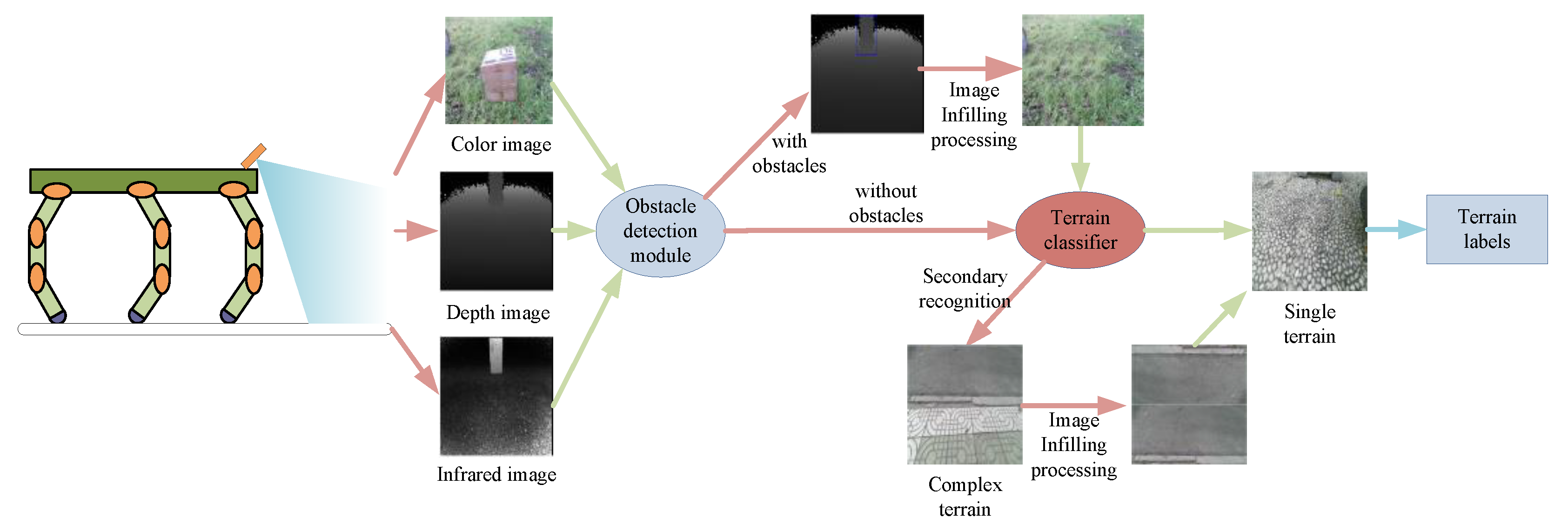
The terrain classification system proposed in this paper is depicted in Figure 2. The Kinect is installed on top of the robot to collect information on terrain (color, depth, and infrared images) and an obstacle detection module is established to detect obstacles in the front. If there are no obstacles, the information will be directly transmitted to the terrain classifier. Otherwise, the module will locate obstacles and identify their size. Meanwhile, a color image of the terrain is processed by the image infilling method to decrease the influence of obstacles on terrain identification. After classification, the confidence scores of each terrain are summarized into a pie chart. The analysis of the pie chart shows whether the terrain is mixed or not. If the terrain is mixed, the color image would be subjected to image segmentation and infilling. Then, the processed color image will be classified by the terrain classifier again, which provides an accurate identification of multiple areas of complex terrain. Finally, all terrain types can be predicted accurately, thus good performance by the robot is guaranteed. The function modules are described in detail in the following section.

2.2.1. Obstacle Detection Module

Detecting and localizing obstacles are important to realize autonomous motion and path planning. The sensors used for traditional obstacle detection mainly include laser radar sensors, ultrasonic sensors, infrared sensors, visual equipment, etc. [24]. In this paper, a fast and accurate detection method based on depth and infrared information is used [25]. The image is segmented by the mean-shift algorithm and the pixel gradient of the foreground is calculated. After pretreatment of edge detection and morphological operation, the depth and infrared information are fused. The characteristics of depth and infrared images are used for edge detection. Thus, the false rate of detection is reduced and detection precision is improved. Since depth images cannot be affected by natural sunlight, the influence of light intensity and shadow on obstacle recognition is effectively eliminated and the robustness of the algorithm is improved. This method can accurately identify the position and size of obstacles. In this paper, the results obtained by obstacle detection with this method are used as the input of the terrain image infilling method.

2.2.2. Terrain Classification Module

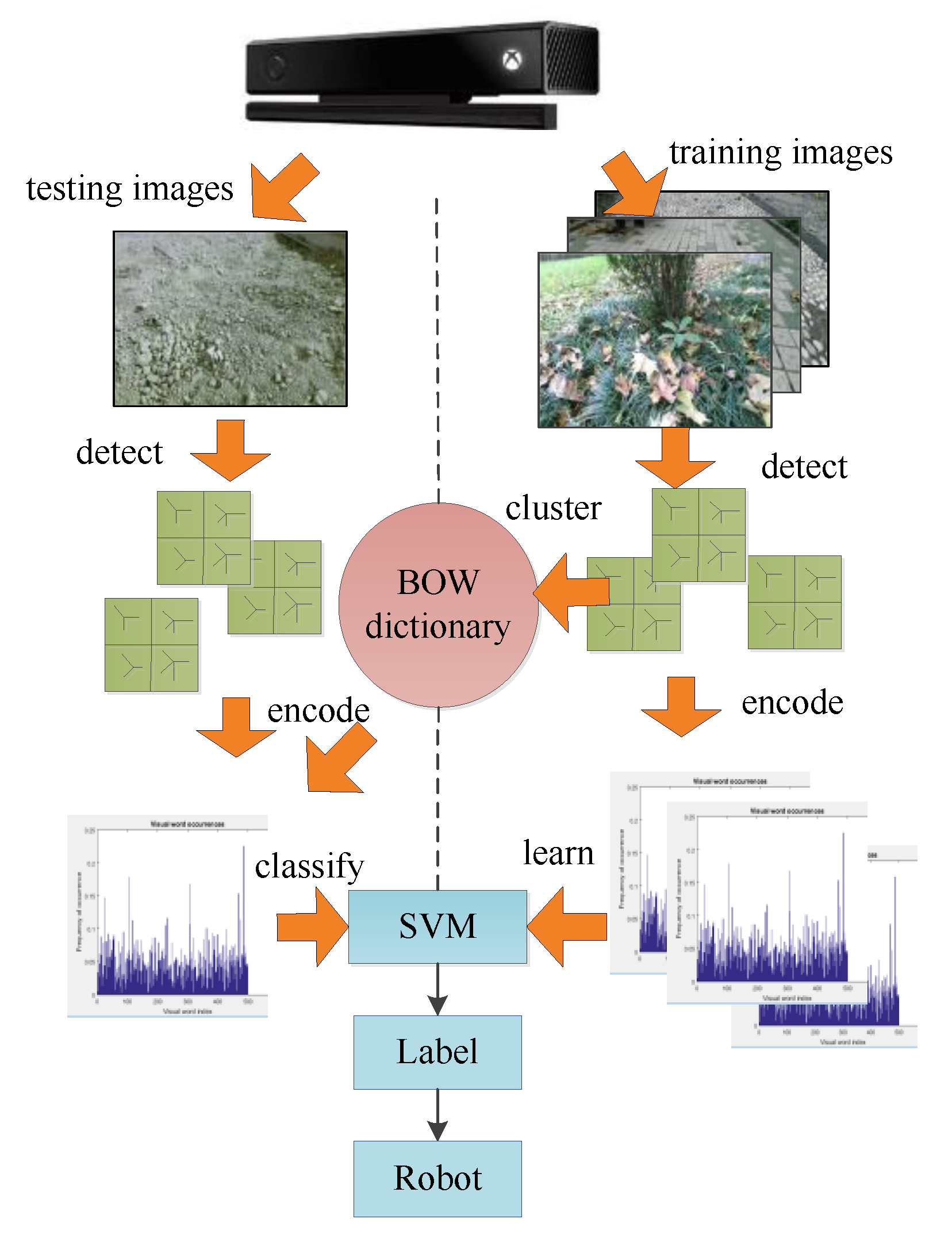
An online terrain classification system is needed to collect information on terrain through the Kinect sensor and then the key points are extracted from a color image of the terrain. Since the terrain classifier is based on the bag-of-words (BoW) module [26], all extracted features are processed by a clustering algorithm to ensure that the clusters have high similarity. These cluster centers are the visual vocabulary. Then, the terrain images are encoded to form the visual dictionary and a visual vocabulary frequency histogram corresponding to each terrain type. Finally, the information is used to train the support vector machine (SVM) [27] and an optimal hyperplane of each terrain type is divided to classify all terrain types. The algorithm can grasp the key samples and eliminate many redundant samples.
The main structure of the terrain classification system is demonstrated in Figure 3. The system is mainly divided into two steps: training and testing. In the first step, the information of all terrain types is collected and stored in memory and the data flow is presented as shown on the right in Figure 3. Then, local features of images in memory are extracted and extracted features are clustered by the k-means algorithm to generate a certain number of visual words [28]. Then, terrain images are encoded using the BoW module to form the visual dictionary and the visual vocabulary frequency histogram corresponding to each terrain type. Then, the information is used to train the SVM. With the aim of validating the terrain classification system established in the training part, the testing part is introduced, shown on the left in Figure 3. The local features from terrain images are extracted in the testing image set and the visual word dictionary is encoded. The images are converted to the frequency histograms that are input in the trained SVM to obtain the terrain label. This part is used by the hexapod robot for terrain recognition. The hexapod robot’s gait transform algorithm is guided by terrain identification.
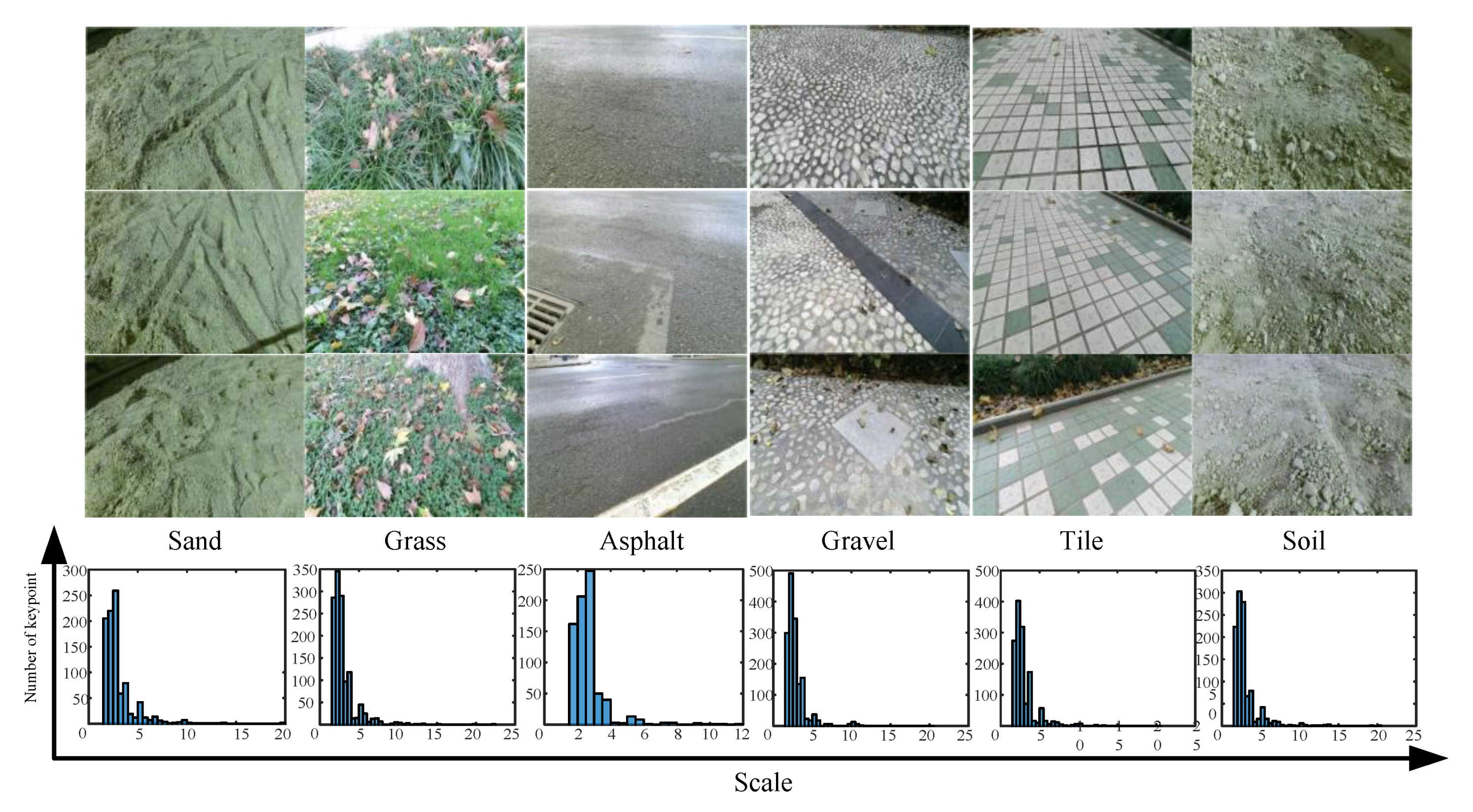
In this paper, a dataset was created using six common terrains: grass, asphalt, sand, gravel, tile, and soil. Each terrain image set contained 50 samples, which were acquired by a Kinect camera. A set of samples of terrain images with different illuminations and weather conditions is shown in Figure 4. The K-fold cross-validation was used and K = 5 [29]. All images were randomly partitioned into five equally sized groups. Each group was chosen as validation data for testing the classifier and other 4 groups for training set.

A. Point of Interesting Extracted by SURF

In the aspect of terrain image feature extraction, the SURF algorithm is a commonly used local feature extraction algorithm in image classification. The matching accuracy is high, but the real-time performance is generally poor. In recent years, many excellent algorithms have been proposed. BRISK [30], which combines detection of key points of features from accelerated segment test (FAST) and binary description can enhance the speed of the algorithm, but its classification performance is not ideal. Since the SURF algorithm with many feature points cannot satisfy real-time detection and the BRISK algorithm has fast computation speed but a low matching rate, a method for image matching based on the SURF-BRISK algorithm is proposed. The SURF-BRISK algorithm is established by combining the advantages of both algorithms. Points of interest are detected using the SURF algorithm, descriptors are calculated using the BRISK algorithm, and the Hamming distance is used [31] for similarity measurement, which enables not only high matching rates but also high calculation speed. The algorithm process is described below. In SURF, the criterion of feature points is the determinant of a Hessian matrix of pixel luminance. A pixel u(x, y) is given in image I. In this point, the scale σ of the matrix is defined by:
H ( μ , σ ) = [ L x x ( u , σ ) L x y ( u , σ ) L x y ( u , σ ) L y y ( u , σ ) ] ,
where Lxx(u,σ) is the Gaussian second-order differential 2 g ( σ ) / x 2 convolution of image I at point u, and similarly for Lxy(u,σ) and Lyy(u,σ). In order to facilitate the calculation, the elements of the Hessian matrix are labeled as Dxx, Dyy, Dxy, and the weight of a square area is set to a fixed value. Hence, the approximate value of the Hessian matrix determinant Happrox is defined by:
det ( H a p p r o x ) = D x x D y y ( ω D x y ) 2 ,
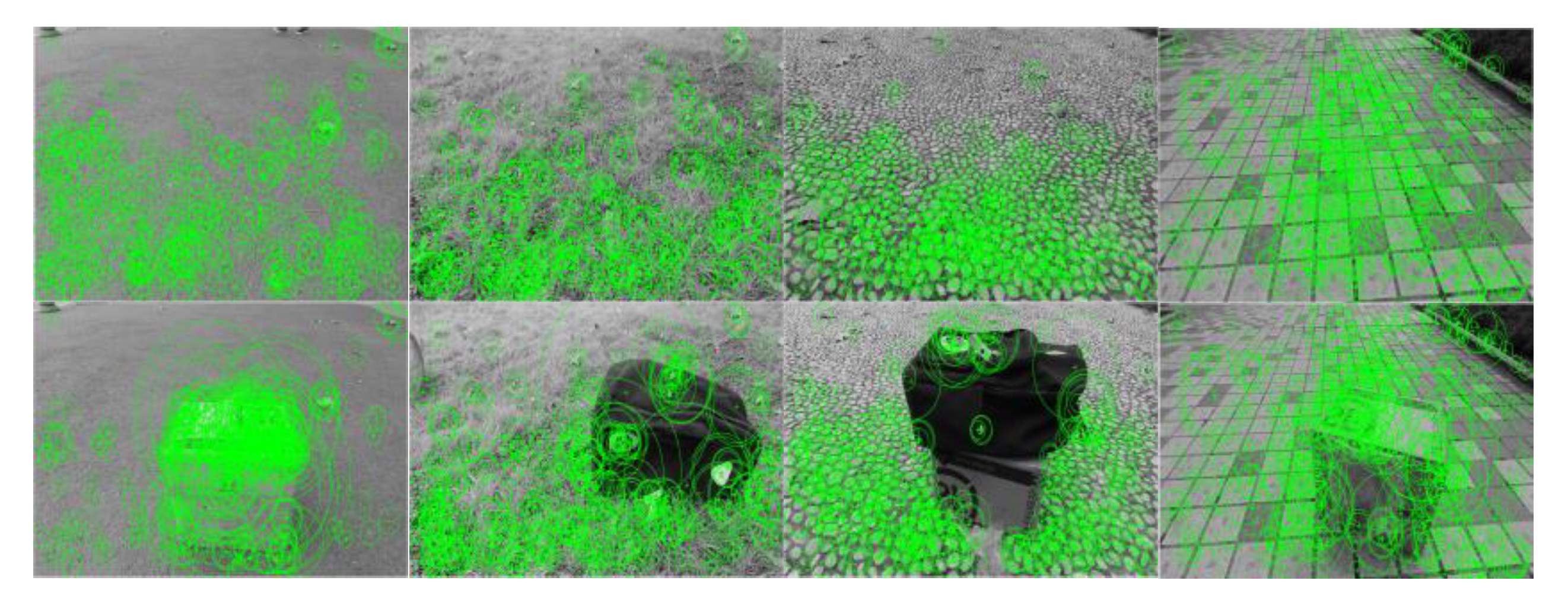
where the correlation weight ω of the filter response is utilized to balance the expression of the Hessian determinant. In order to preserve the energy conservation of the Gauss kernel and approximate it, ω is usually set to 0.9. The Hessian matrix is used to calculate the partial derivative, which is usually obtained by a convolution of pixel light intensity and a certain direction of Gauss kernel partial derivative. In order to improve the speed of the SURF algorithm, the approximate box filter is used instead of the Gauss kernel with very little impact on precision. The convolution calculation can be used to optimize the integral image, which greatly improves the efficiency. It is necessary to use three filters to calculate Dxx, Dyy, and Dxy for each point. After filtering, a response graph of the image is obtained. The value of each pixel on the response graph is calculated by the determinant of the original pixel. The image is filtered with different scales and a series of responses of the same image at different scales is obtained. The detection method of feature points is if the value of det (Happrox) of a key point is greater than the value of 26 points in its neighborhood. The number of interest points sampled by SURF is shown in Figure 4.

B. Descriptors by BRISK

The BRISK descriptor adopts the neighborhood sampling model, which takes the feature points as the center of the circle. The points on the concentric circles of several radii are selected as the sampling points. In order to reduce the effect caused by sample image grayscale aliasing, the Gauss function can be used for filtering. The Gauss function of standard deviation sigma is proportional to the distance between the points on each concentric circle. Selecting a pair from the point pairs formed by all sampling points, denoted as (Pi, Pj), the gray values after treatment are I(Pi, σi) and I(Pjj), respectively. Hence, the gradient between two sampling points is
g ( P i , P j ) = ( P j P i ) I ( P j , σ j ) I ( P i , σ i ) P j P i 2 .
Set A is a collection of all pairs of sampling points, S is a set containing all the short-range sampling pairs, and L is a set containing all the long-distance pairs of sampling points:
A = { ( P i , P j ) R 2 × R 2 | i < N j < i i , j N } ,
S = { ( P i , P j ) A | P j P i < δ max } A ,
L = { ( P i , P j ) A | P j P i < δ min } A .
The general distance thresholds δmax = 9.75 t, δmin = 13.67 t, and t are characteristic point scales. The main direction for each feature point is specified by the gradient direction distribution characteristics of neighboring pixels of the feature point. In general, the BRISK algorithm can be used to solve for the direction g of the overall pattern according to the gradient between two sampling points:
g = ( g x g y ) = 1 L ( P i , P j ) L g ( P i , P j ) .
In order to achieve rotation and scale invariance, the sampling pattern is sampled again after the rotation angle θ = arctan2 (gy, gx). The binary descriptor b can be constructed by performing Equation (8) on all pairs of points in set S by short-range sampling points.
b = { 1 0 I ( P j θ , σ j ) > I ( P i θ , σ i ) o t h e r w i s e ( P i θ , P j θ ) S

C. Local Feature Matching

After the feature descriptors extracted by SURF-BRISK are 512-bit binary bit strings consisting of 0 and 1, the Hamming distance is used to measure similarity. Assuming that there are two descriptors of S1 and S2, the Hamming distance is determined as
D k d ( S 1 , S 2 ) = i = 1 512 ( x i y i ) ,
where S1 = x1x1 … x512, S2 = y1y2 … y512, x, y and the value of x and y is 0 or 1. The smaller the value of Dkd, the higher the matching rate, and vice versa. Therefore, the matching point pairs are obtained using the nearest-neighbor Hamming distance in the matching process.
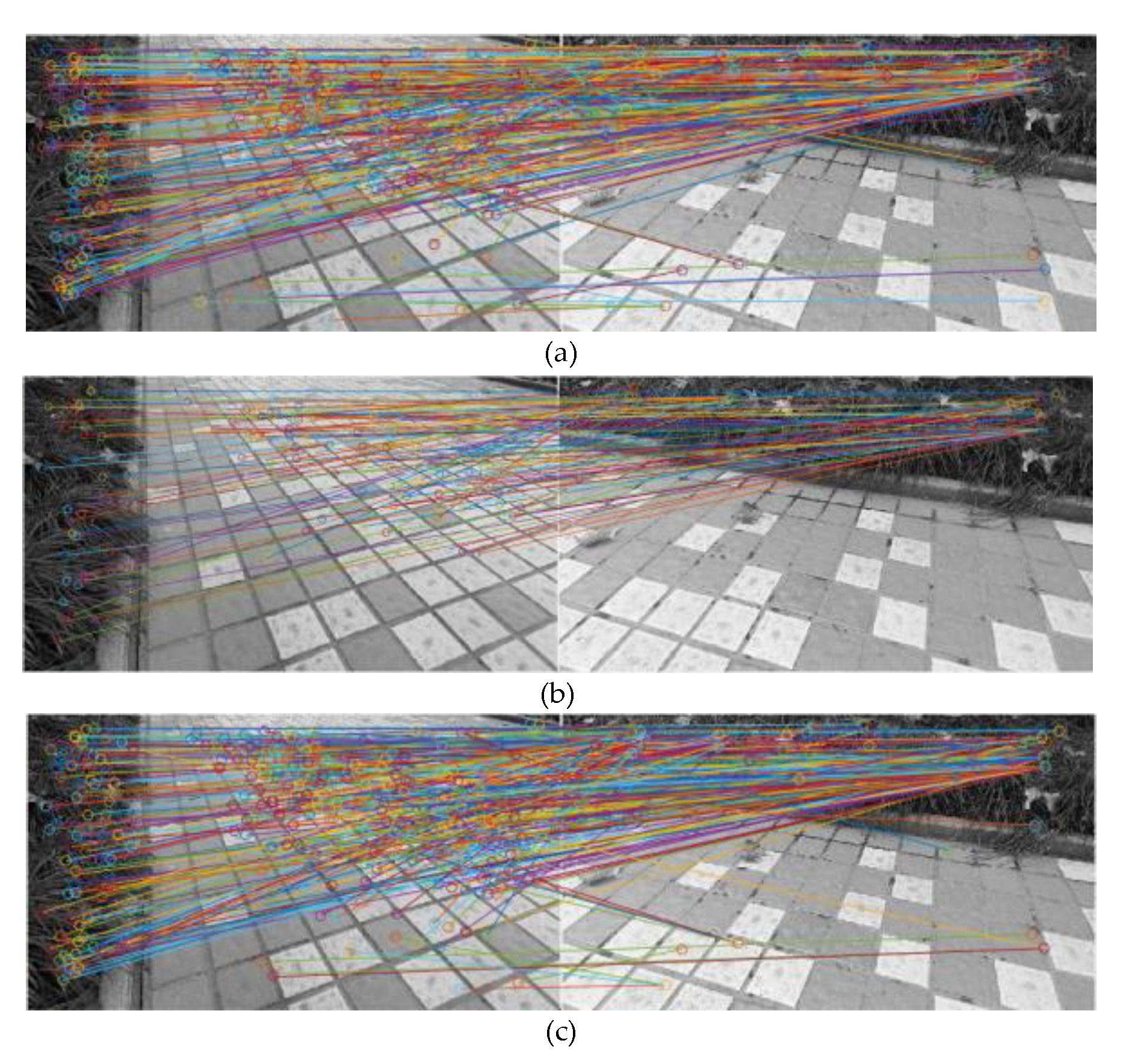
Here, three descriptors, SURF, BRISK, and SURF-BRISK, are compared. Two tile images have been chosen for matching tests to compare the real-time and matching rate of these descriptors, as shown in Table 1 and Figure 5. Obviously, the SURF algorithm has the most matching points, the BRISK algorithm has the fastest matching, and the SURF-BRISK algorithm combines the advantages of both. The algorithm is faster than SURF and gets more matching points than BRISK.

D. BoW Model and SVM

Li et al. [32] first introduced the image method based on the BoW model. They believed that an image can be analogized to a document and the “words” of an image can be defined as feature vectors. The basic BoW model regards an image as a set of feature vectors and statistics of occurrence frequency of feature vectors, which are used for terrain classification. The BoW model can be set up by a clustering algorithm that is used to obtain the visual dictionary and the steps are as follows. Feature extraction: m images (m ≥ 50) are collected for each terrain type and each image is extracted by SURF-BRISK to obtain n(i) feature vectors. All terrain images form a total sum (n(i)) of feature vectors (words). Generation of dictionary/codebook: The feature vectors obtained from the previous step are clustered (here, the k-means clustering method is used [33]) to get k clustering centers in order to build the codebook. A histogram is generated according to the codebook. The nearest neighbor calculation of each word of the picture is used to find the corresponding words in the codebook in order to form the BoW model.
SVM is an excellent learning algorithm developed on the basis of statistics theory and is widely used in many fields, such as image classification, handwriting recognition, and bioinformatics. The input vector is mapped to a high-dimensional feature space by nonlinear mapping (a kernel function) and an optimal hyperplane is constructed in this space. Compared with the artificial neural network, which suffers from an overfitting problem, the support vector machine has better generalization ability for unknown samples [34]. SVM can be divided into three groups: linear separable, nonlinear separable, and kernel function mapping. Linear classifier performance is limited to linear problems, because in nonlinear problems constraints of excessive relaxation can lead to a large number of error samples. At this point, it can be transformed into a linear problem in a high-dimensional space using nonlinear transformation in order to obtain an optimal classification hyperplane.

2.3. Complex Terrain Recognition

In the field, terrain is usually complex. The accuracy of terrain with obstacles and mixed terrain, which is composed of two or more terrain types, is greatly reduced if traditional identification methods are used. This scenario affects the normal operation of the robot. Therefore, a systematic method based on image segmentation and infilling for recognition of terrain with obstacles and mixed terrain is introduced in this section.

2.3.1. Image Local Infilling for Terrain with Obstacles

Information on terrain with obstacles collected by Kinect is used as input data for the terrain classifier. It was found that large-volume obstacles cause low accuracy of final identification, because acquired features of terrain information are severely affected, since SURF-BRISK and SURF have the same points of interest. The distributions of points in different terrains with and without obstacles are shown in Figure 6. The obstacles greatly influence local feature extraction. In order to improve the accuracy of recognizing terrain with obstacles, a method of image local infilling (ILI) is presented. The errors for terrain with obstacles in the first round of recognition are shown in Table 2.
The obstacle area of pixel matrix I(m, n) is obtained using the obstacle detection method, as are the central pixel coordinates (u, v). Here, three infilling examples are illustrated for comparison. The obstacle area with a pixel value of I = 255 is presented as a white area in Figure 7b. The obstacle area with a pixel value of I = 0 is presented as a black area in Figure 7c. The obstacle area spliced by the no-obstacle sides of the background terrain image is presented in Figure 7d. Due to the use of both left and right sides of the terrain image for infilling, it only needs to compare the abscissa u of the obstacle area center and the abscissa uc of the color image center. At the same time, according to the dimensions of I(m, n), the size and orientation of obstacles are determined. If the width of the obstacle area, i.e., the number n of matrix I(m, n), is too large, the image needs to be processed by multiple infilling. The classification and statistical results of the terrain classifier after ILI are also shown in Table 2. The first two methods do not improve the accuracy of image recognition, since white and black features do not contribute to the main feature points. However, the background terrain–based image infilling shows satisfactory results.

2.3.2. Image Infilling for Mixed Terrain

After the first round of classification, both the terrain label and confidence score of the classified image are obtained. In SVM, the confidence score represents the geometric interval between the classified image and the hyperplane of each terrain type. Therefore, the confidence score needs to be normalized before conducting an analysis. The confidence score is adjusted to the interval [0, 1] to facilitate the comparison. Set Sd contains the confidence scores of all terrain types, and di is the confidence of the test image that corresponds to i terrain class before normalization. Set SD contains confidence scores after normalization and Di is normalized confidence. Therefore, after normalization we get
S D = { D i | D i = | d i | / i = 1 6 | d i | , i = 1 , 2 , , 6 } .
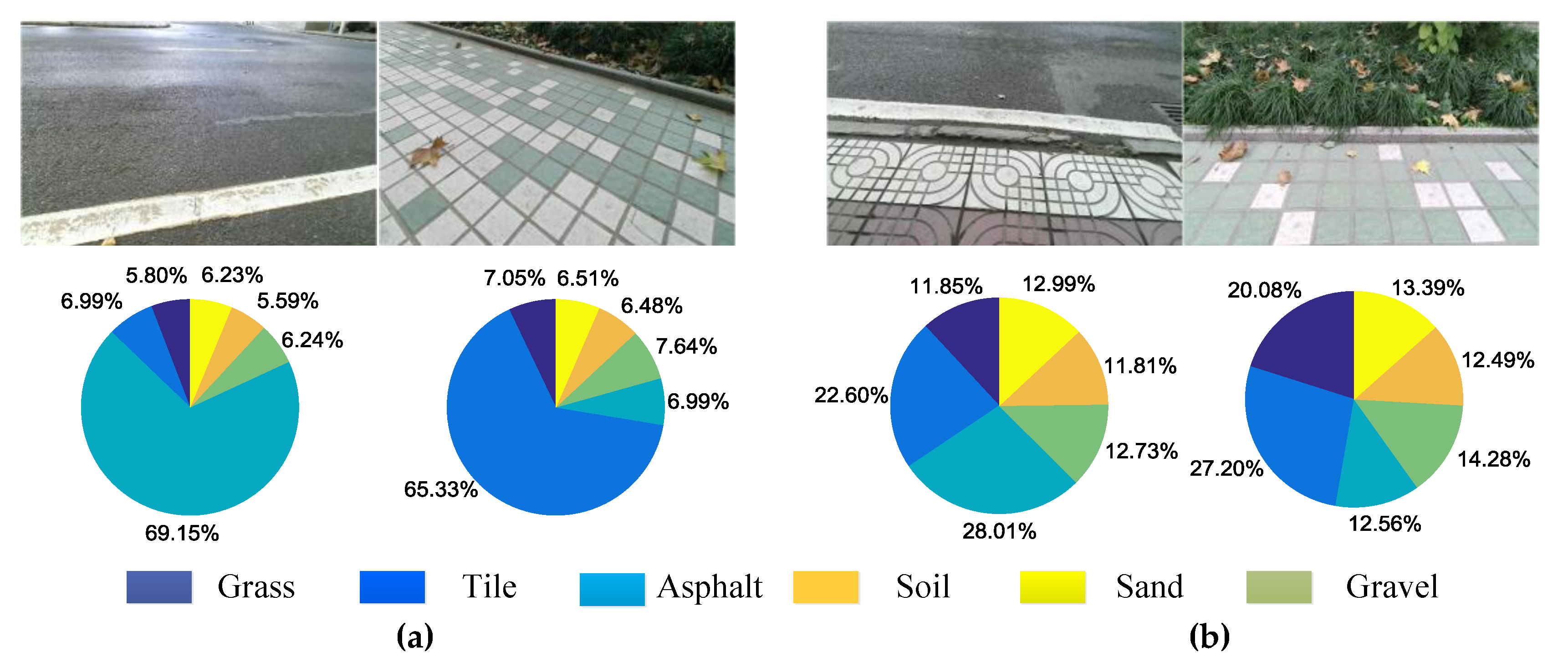
Moreover, a pie chart of confidence scores after normalization can clearly demonstrate the contribution of each terrain type. A pie chart of confidence scores after the first round of classification is shown in Figure 8. In the images of single terrain, the weight of single terrain is much higher than the weights of other terrains. A series of experiments demonstrated that if the highest terrain weight is larger than 30% and more than 10% higher than the second highest weight, the terrain can be considered as a single terrain. Otherwise, it is mixed terrain. For mixed terrain, it is difficult to identify the category from weights in the pie chart. In addition, it is important to note that mixed terrain usually appears at the intersection of different terrains. The traditional methods are not practical for images that contain two or more terrain types, because only one label will be notified. Obviously, some approaches can identify the boundaries of different terrains in an image and then make the decision. Actually, it is difficult to accurately determine terrain boundaries and the algorithm needs to do many computations, which causes poor real-time performance that affects the robot’s outdoor walking. In the process of the robot moving in a forward direction, the terrain type is gradually changing. Different types of terrain appear in up and down form in the images. Taking this into consideration, a new method for identification of mixed terrain based on super-pixel image infilling (SPI) is presented.
In the field of image segmentation, super-pixel has become a fast-developing image preprocessing technology. Ren et al. [35] first proposed the concept of super-pixels, which quickly divide images into a number of subareas that have image semantics. Compared with the traditional processing method, the extraction and expression of super-pixels are more conducive to collecting local characteristics of the image information. It can greatly reduce the calculation and subsequent processing complexity. Existing segmentation algorithms generally restrict the number of pixels, the compactness, the quality of segmentation, and the practicability of algorithms. Song et al. [36] evaluated the existing super-pixel segmentation algorithms. Their results indicate that the simple linear iterative cluster (SLIC) super-pixel segmentation algorithm has good performance in terms of the controllability of pixel numbers and the close degree of controllability. Aiming at segmentation, the SLIC algorithm is used for mixed terrain regions. The most super-pixels are selected as the target area in a multi-super-pixel area and the boundary pixels of the pixel coordinates of curve fitting are extracted as the terrain boundary segmentation of a complex terrain image. The procedure and results are shown in Figure 9.
Classification results after image segmentation are shown in Table 3. The output labels do not match actual terrain types. For this mismatch, the number of points of interest extracted from segmented images is shown in Figure 10. Compared with the original terrain image in Figure 4, the number of feature points of segmented images is still related to terrain type but much smaller. Obviously, it is impossible to realize an accurate prediction using the segmentation image, because the feature points are inadequate. Thus, the segmented images are spliced together to enhance the terrain features. Segmented color images would have only some of the pixels of the original color image collected by the Kinect camera and the blank pixels would be infilled by duplication of the segmented image. In the test, the rotation–inversion operation is used for image infilling. The results are shown in Figure 11.
The number of feature points in Figure 10 and Figure 11 shows that the proposed method can enhance local features of segmented images. The classification results of a spliced image using this approach are shown in Table 3. Using the image infilling approach (rotation–inversion), the error results of the first-round classification can be corrected. It can be seen that confidence scores of the correct terrain type increased after image infilling. On the contrary, confidence scores of wrong terrain types decreased. That means the proposed method can effectively magnify image features for the classifier.

3. Results

3.1. Complex Terrain

In the experiments, the hexapod robot walked on six types of terrain without obstacles. Terrain images were collected by a Kinect camera installed on top of the robot. The inclination angle of the Kinect sensor is 40°. Images of terrain with obstacles were collected at different times and in different weather and light conditions. Obstacles mainly included cartons, trash, trees, and so on. There were 50 images collected for each terrain type. The collected images of terrain with obstacles were processed by the ILI method. Then, all images before and after ILI processing were classified by the presented terrain classifier. The recognition results for the two sets are shown in Figure 12a. The recognition rate of terrain with obstacles before ILI processing was relatively low. Since obstacles seriously affect local features of the terrain, error exists in most cases and average recognition accuracy is less than 75%. On the contrary, after the image infilling process, recognition accuracy was improved to above 85%.
Usually, mixed terrain appears at the intersection of different terrains. All mixed terrain images were collected at that moment. Specifically, 50 images were collected and processed by the SPI method for terrain recognition. The result is shown in Figure 12b. The classifier shows the labels of two terrain types for different subareas in the image. The average recognition accuracy reached 85% and the results show that the proposed method is effective in recognizing mixed terrain. At the same time, compared with a single label classifier, the SPI method has more practical significance for gait transition of the hexapod robot.

3.2. Robot Platform Application

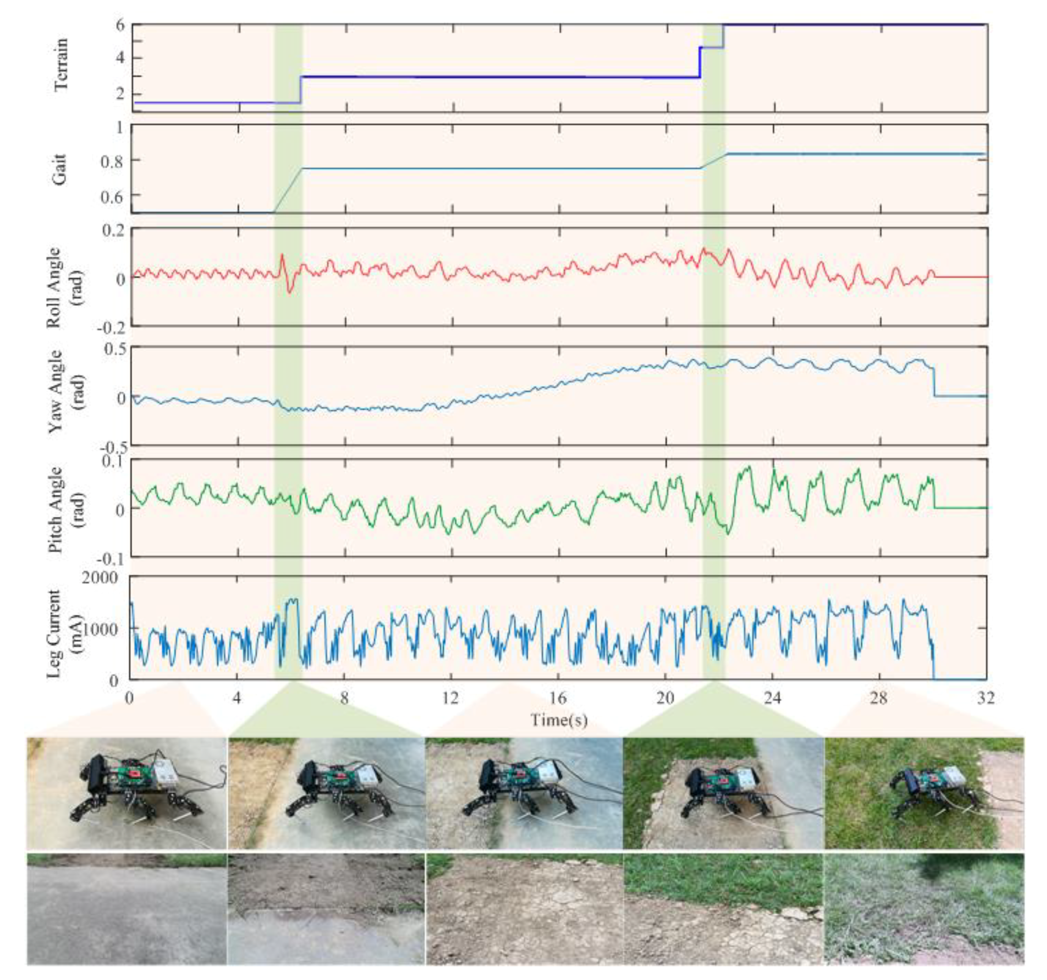
When the robot walks on different terrains, different gaits have different effects on the robot’s stability, performance, and energy consumption. The experiment showed that the gait can be changed based on the output of the terrain classifier. In the experiment, the hexapod robot walked for 30 s across three terrain types: asphalt, soil, and grass. The sampling period of the Kinect is 1 s. The gait pattern of the hexapod robot was set according to the output of the terrain classifier. The pseudocode of the gait transition algorithm is depicted in Table 4.
The value of G has a great influence on the smoothness and efficiency of motion on different terrains. The terrain classification results, including gait value, leg current from robot legs SRL1, and attitude angle, are shown in Figure 13. From 0–5 s, the terrain is supposed to be asphalt. Thus, the robot moves in tripod gait. From 5–6 s, the robot is in transition gait and ready to stride across mixed terrain consisting of asphalt and soil. The value of the terrain curve is nominal, showing that the terrain is complex, e.g., 1.3 means the terrain is changing from type 1 to type 3. From 6–21 s, the robot moves forward with its current gait. Then, from 22–23 s, it changes gait to get ready for another terrain. Finally, from 23–30 s, the terrain is grass and the robot continues to move in a wave gait. The experimental results show that the robot can walk stably on a single-terrain type and transform its gait successfully according to different terrains. At the initial moment, captured images from the Kinect are classified by system. The confidence rating of the classified asphalt is greater than 30%, so the terrain image is judged by the system to be asphalt pavement in a single terrain. Similarly, at 14 s and 22 s, the system outputs a single terrain label for soil and grass. At 5 s and 22 s, the terrain image corresponds to the uncertain category and the highest confidence is less than 30%. Therefore, the terrain is supposed to be mixed, and image infilling method is used until the classification result meets recognition reliability requirements. The system outputs the labels of two terrains and causes the robot to make the corresponding gait transitions.

4. Discussion

This paper describes a terrain classification system for a multilegged robot on complex terrain with obstacles. Several topographic classification methods are summarized in Table 5 [8,11,17,37,38,39,40,41]. With respect to single terrain recognition, several successful single terrain classification methods proved the effectiveness of this kind of methodology via local features, BoW model, and SVM. The common points (also advantages) of these works and our proposed algorithm include the following: Image features are extracted by selecting local features. Unlike color-based and spectra-based methods, local features are invariant to scale, rotation, brightness, and contrast and hence have become popular in image classification. In these methods, the SURF algorithm is used to extract local features of terrain images as input to the BoW model. The performance of SVM in classifying a small number of samples is also excellent. The characteristics of sensor-based information including frequency of leg current [38] and tactile data [40] are also used for terrain recognition. This kind of data is similar in the same terrain and has certain regularity in different terrains. The methods of building the classifier mainly focus on SVM [8,11,17], neural network [37,38,39], and mixtures of Gaussians [40,41]. Among them, SVM and neural network are the two main classification models. The application of terrain identification to legged robots is mainly concentrated on gait transition and path planning. For terrain classification with a multilegged robot, the precision requirement is low and a simple SVM is good enough for expected results. Our image infilling algorithm has the effect of magnifying local features of the image, which makes the classification more accurate. We also made an innovation in feature extraction: the SURF-BRISK algorithm is more suitable for real-time classification, its matching speed is much faster than the SURF algorithm alone, and its accuracy is also in line with the SURF algorithm.

5. Conclusions

In this paper, a novel terrain classification system for accurate recognition of different terrains is proposed. By using Kinect, color, infrared, and depth images are acquired simultaneously. The infrared and depth information are fused and used for obstacle detection. The local feature extraction of terrain images is done by the SURF-BRISK algorithm. A terrain classifier based on the BoW model and SVM is employed. Using the proposed method, different terrains can be classified quickly and precisely. Complex terrain recognition is achieved by the local image infilling method for terrain with obstacles and mixed terrain. According to the experimental results, the proposed method greatly improves the accuracy of complex terrain recognition and plays an important role in locomotion guidance of multilegged robots.
The theoretical contributions and novelty of this paper can be summarized as follows:
(1) Images with obstacles are infilled by surrounding terrain parts in order to improve the classification accuracy. Thus, the local features of images are magnified and the method can achieve satisfactory results.
(2) A super-pixel image infilling method for mixed terrain classification is presented. The average classification accuracy of the proposed method for mixed terrain is over 80%. The proposed method can make acquired data more believable and reliable for locomotion planning and control of intelligent robots.
(3) Multiple terrain labels can be given instead of a single label, which indicates that the presented method is very practical for complex terrains.
This paper focuses on a complex terrain classification system and a combination of terrain classification and obstacle detection to complete the planning of a robot path. In the future, we will improve the rapid transformation of a robot’s gait based on terrain information and make the robot more intelligent.

Author Contributions

Y.Z. designed the algorithm. Y.Z., C.M., C.J., and Q.L. designed and carried out the experiments. Y.Z. and C.J. analyzed the experimental data and wrote the paper. Q.L. gave many meaningful suggestions about the structure of the paper.

Funding

This research was funded by the National Natural Science Foundation of China (No. 51605039), the Thirteenth Five-Year Plan Equipment Pre-research Field Fund (No. 61403120407), the China Postdoctoral Science Foundation (No. 2018T111005 and 2016M592728), Fundamental Research Funds for the Central Universities, CHD (No. 300102259308, 300102258203 and 300102259401).

Conflicts of Interest

The authors declare no conflict of interest.

References

  1. Yu, Z.; Chen, J.; Dai, Z. Study on Forces Simulation of Gecko Robot Moving on the Ceiling. Adv. Intell. Soft Comput. 2012, 125, 81–88. [Google Scholar] [CrossRef]
  2. Abbaspour, R. Design and Implementation of Multi-Sensor Based Autonomous Minesweeping Robot. In Proceedings of the International Congress on Ultra Modern Telecommunications & Control Systems & Workshops, Moscow, Russia, 18–20 October 2010; IEEE: Piscataway, NJ, USA, 2010; pp. 443–449. [Google Scholar] [CrossRef]
  3. Ayers, J. Localization and Self-Calibration of a Robot for Volcano Exploration. In Proceedings of the ICRA 04 2004 IEEE International Conference on Robotics and Automation, New Orleans, LA, USA, 26 April–1 May 2004; IEEE: Piscataway, NJ, USA, 2004; Volume 1, pp. 586–591. [Google Scholar] [CrossRef]
  4. Zhao, S.D.; Yuh, J.K. Experimental Study on Advanced Underwater Robot Control. IEEE Trans. Robot. 2005, 21, 695–703. [Google Scholar] [CrossRef]
  5. Cui, Y.; Gejima, Y.; Kobayashi, T. Study on Cartesian-Type Strawberry-Harvesting Robot. Sens. Lett. 2013, 11, 1223–1228. [Google Scholar] [CrossRef]
  6. Semler, L.; Furst, J. Wavelet-Based Texture Classification of Tissues in Computed Tomography. In Proceedings of the IEEE International Conference on Image Processing, Atlanta, GA, USA, 8–11 October 2006; IEEE: Piscataway, NJ, USA, 2006; pp. 265–270. [Google Scholar]
  7. Paschos, G. Perceptually uniform color spaces for color texture analysis: An empirical evaluation. IEEE Trans. Image Proc. 2001, 10, 932–937. [Google Scholar] [CrossRef]
  8. Liu, X.; Wang, D. Texture classification using spectral histograms. IEEE Trans. Image Proc. 2003, 6, 661–670. [Google Scholar] [CrossRef]
  9. Pietikäinen, M.; Mäenpää, T.; Viertola, J. Color Texture Classification with Color Histograms and Local Binary Patterns; IWTAS: New York, NY, USA, 2002; pp. 109–112. [Google Scholar]
  10. Zenker, S.; Aksoy, E.E.; Goldschmidt, D. Visual Terrain Classification for Selecting Energy Efficient Gaits of a Hexapod Robot. In Proceedings of the IEEE/ASME International Conference, Wollongong, Australia, 9–12 July 2013; IEEE: Piscataway, NJ, USA; Advanced Intelligent Mechatronics (AIM): Marseille, France, 2013; pp. 577–584. [Google Scholar] [CrossRef]
  11. Khan, Y.; Komma, P.; Bohlmann, K. Grid-Based Visual Terrain Classification for Outdoor Robots Using Local Features. In Proceedings of the IEEE Symposium on Computational Intelligence in Vehicles and Transportation Systems, Paris, France, 11–15 April 2011; IEEE: Piscataway, NJ, USA, 2011; pp. 16–22. [Google Scholar] [CrossRef]
  12. Kim, J.; Kim, D.; Lee, D. Non-contact Terrain Classification for Autonomous Mobile Robot. In Proceedings of the IEEE International Conference on Robotics and Biomimetics, Guilin, China, 19–23 December 2009; IEEE: Piscataway, NJ, USA, 2009; pp. 824–829. [Google Scholar] [CrossRef]
  13. Ojeda, L.; Borenstein, J.; Witus, G.; Karlsen, R. Terrain characterization and classification with a mobile robot. J. Field Robot. 2006, 9, 103–122. [Google Scholar] [CrossRef]
  14. Larson, A.C.; Voyles, R.M.; Bae, J. Evolving Gaits for Increased Selectivity in Terrain Classification. In Proceedings of the IEEE/RSJ International Conference on Intelligent Robots and Systems, Sheraton Hotel and Marina, San Diego, CA, USA, 29 October–2 November 2007; IEEE: Piscataway, NJ, USA, 2007; pp. 3691–3696. [Google Scholar] [CrossRef]
  15. Hoepflingen, M.A.; Remy, C.D.; Hutter, M. Terrain Classification for Legged Robots. In Proceedings of the IEEE International Conference on Robotics and Automation, ICRA 2010, Anchorage, AK, USA, 3–7 May 2010; IEEE: Piscataway, NJ, USA, 2010; pp. 2828–2833. [Google Scholar] [CrossRef]
  16. Jitpakdee, R.; Maneewam, T. Neural Networks Terrain Classification Using Inertial Measurement Unit for an Autonomous Vehicle. In Proceedings of the SICE Annual Conference, Tokyo, Japan, 20–22 August 2008; IEEE: Piscataway, NJ, USA, 2008; pp. 554–558. [Google Scholar] [CrossRef]
  17. Filitchkin, P.; Byl, K. Feature-Based Terrain Classification for LittleDog. In Proceedings of the 2012 IEEE/RSJ International Conference on Intelligent Robots and Systems (IROS), Vilamoura, Portugal, 7–12 October 2012; IEEE: Piscataway, NJ, USA, 2012; pp. 1387–1392. [Google Scholar] [CrossRef]
  18. Zuo, L.; Wang, M.; Yang, Y. Complex Terrain Classification algorithm Based on Multi-Sensors Fusion. In Proceedings of the 32nd Chinese Control Conference (CCC), Xi’an, China, 26–28 July 2013; Inspec Accession Number: 13886652. pp. 5722–5727. [Google Scholar]
  19. Ugur, E.; Dogar, M.R.; Cakmak, M.; Sahin, E. The learning and use of traversability affordance using range images on a mobile robot. In Proceedings of the 2007 IEEE International Conference on Robotics and Automation, Roma, Italy, 10–14 April 2007; IEEE: Piscataway, NJ, USA, 2007. [Google Scholar] [CrossRef]
  20. Zhu, Y.G.; Jin, B. Trajectory Correction and Locomotion Analysis of a Hexapod Walking Robot with Semi-Round Rigid Feet. Sensors 2016, 9, 1392. [Google Scholar] [CrossRef] [PubMed]
  21. Zhu, Y.G.; Jin, B. Compliance control of a legged robot based on improved adaptive control: Method and experiments. Int. J. Robot. Autom. 2016, 5, 366–373. [Google Scholar] [CrossRef]
  22. Zhu, Y.G.; Wu, Y.S.; Liu, Q.; Guo, T.; Qin, R.; Hui, J.Z. A backward control based on σ -Hopf oscillator with decoupled parameters for smooth locomotion of bio-inspired legged robot. Robot. Auton. Syst. 2018, 106, 165–178. [Google Scholar] [CrossRef]
  23. Zhu, Y.G.; Guo, T.; Liu, Q.; Zhu, Q.; Zhao, X.; Jin, B. Turning and Radius Deviation Correction for a Hexapod Walking Robot Based on an Ant-Inspired Sensory Strategy. Sensors 2017, 17, 2710. [Google Scholar] [CrossRef]
  24. Discant, A.; Rogozan, A. Sensors for Obstacle Detection a Survey. In Proceedings of the 30th International Spring Seminar on the Electronics Technology, Cluj-Napoca, Romania, 9–13 May 2007; IEEE: Piscataway, NJ, USA, 2007; pp. 100–105. [Google Scholar] [CrossRef]
  25. Zhu, Y.G.; Yi, B.M.; Guo, T. A Simple Outdoor Environment Obstacle Detection Method Based on Information Fusion of Depth and Infrared. J. Robot. 2016, 9, 1–10. [Google Scholar] [CrossRef]
  26. Comaniciu, D.; Meer, P. Mean shift: A robust approach toward feature space analysis. IEEE Trans. Pattern Anal. Mach. Intell. 2002, 5, 603–619. [Google Scholar] [CrossRef]
  27. Comaniciu, D. Rr Vision and Pattern Recognition. In Proceedings of the Conference on Computer Vision and Pattern Recognition, Hilton Head Island, SC, USA, 15 June 2000; IEEE: Piscataway, NJ, USA, 2000; pp. 142–149. [Google Scholar] [CrossRef]
  28. Qin, L. Category Related BoW Model for Image Classification. J. Inf. Comput. Sci. 2015, 9, 3547–3554. [Google Scholar] [CrossRef]
  29. Yadav, S.; Shukla, S. Analysis of k-Fold Cross-Validation over Hold-Out Validation on Colossal Datasets for Quality Classification. In Proceedings of the IEEE International Conference on Advanced Computing, Bhimavaram, India, 27–28 February 2016; IEEE: Piscataway, NJ, USA, 2016; pp. 71–83. [Google Scholar] [CrossRef]
  30. Leutenegger, S.; Chli, M.; Siegwart, R. BRISK: Binary Robust Invariant Scalable Keypoints. In Proceedings of the 2011 IEEE International Conference on Computer Vision-ICCV, Barcelona, Spain, 6–13 November 2011; IEEE: Piscataway, NJ, USA, 2011; Volume 11, pp. 2548–2555. [Google Scholar] [CrossRef]
  31. Cui, Z.; Li, Z. Two kinds of improved template matching recognition algorithm. Comput. Eng. Des. 2006, 6, 1083–1084. [Google Scholar]
  32. Fei-Fei, L.; Perona, P. A Bayesian Hierarchical Model for Learning Natural Scene Categories. In Proceedings of the Conference on IEEE Computer Vision and Pattern Recognition, San Diego, CA, USA, 20–26 June 2005; IEEE Computer Society: Washington, DC, USA, 2005; pp. 524–531. [Google Scholar] [CrossRef]
  33. Wang, Q.; Wang, C. Review of k-means algorithm for clustering. Electr. Des. Eng. 2014, 6, 479–484. [Google Scholar]
  34. Chapelle, O. Training a Support Vector Machine in the Primal. Neural Comput. 2007, 19, 1155–1178. [Google Scholar] [CrossRef] [Green Version]
  35. Ren, X.; Malik, J. Learning a Classification Model for Segmentation. In Proceedings of the IEEE International Conference on Computer Vision, Nice, France, 13–16 October 2003; IEEE: Piscataway, NJ, USA, 2003; pp. 11–17. [Google Scholar] [CrossRef]
  36. Song, X.; Zhou, L.; Li, Z. Review on superpixel methods in image segmentation. J. Image Gr. 2015, 20, 599–608. [Google Scholar]
  37. Lee, S.Y.; Kwak, D.M. A terrain Classification Method for UGV Autonomous Navigation Based on SURF. In Proceedings of the International Conference on Ubiquitous Robots & Ambient Intelligence, Incheon, Korea, 23–26 November 2011; IEEE: Piscataway, NJ, USA, 2011; pp. 303–306. [Google Scholar] [CrossRef]
  38. Ordonez, C. Terrain identification for R Hex-type robots. Unmanned Syst. Technol. XV 2013, 3, 292–298. [Google Scholar] [CrossRef]
  39. Holder, C.J.; Breckon, T.P. From On-Road to Off: Transfer Learning Within a Deep Convolutional Neural Network for Segmentation and Classification of Off-Road Scenes. Springer Int. Publ. 2016, 9, 149–162. [Google Scholar] [CrossRef]
  40. Dallaire, P. Learning Terrain Types with the Pitman-Yor Process Mixtures of Gaussians for a Legged Robot. In Proceedings of the 2015 IEEE/RSJ International Conference on Intelligent Robots and Systems (IROS), Hamburg, Germany, 28 September–2 October 2015; IEEE: Piscataway, NJ, USA, 2015; pp. 3457–3463. [Google Scholar] [CrossRef]
  41. Manduchi, R.; Castano, A.; Talukder, A. Obstacle Detection and Terrain Classification for Autonomous Off-Road Navigation. Auton. Robots 2005, 1, 81–102. [Google Scholar] [CrossRef]
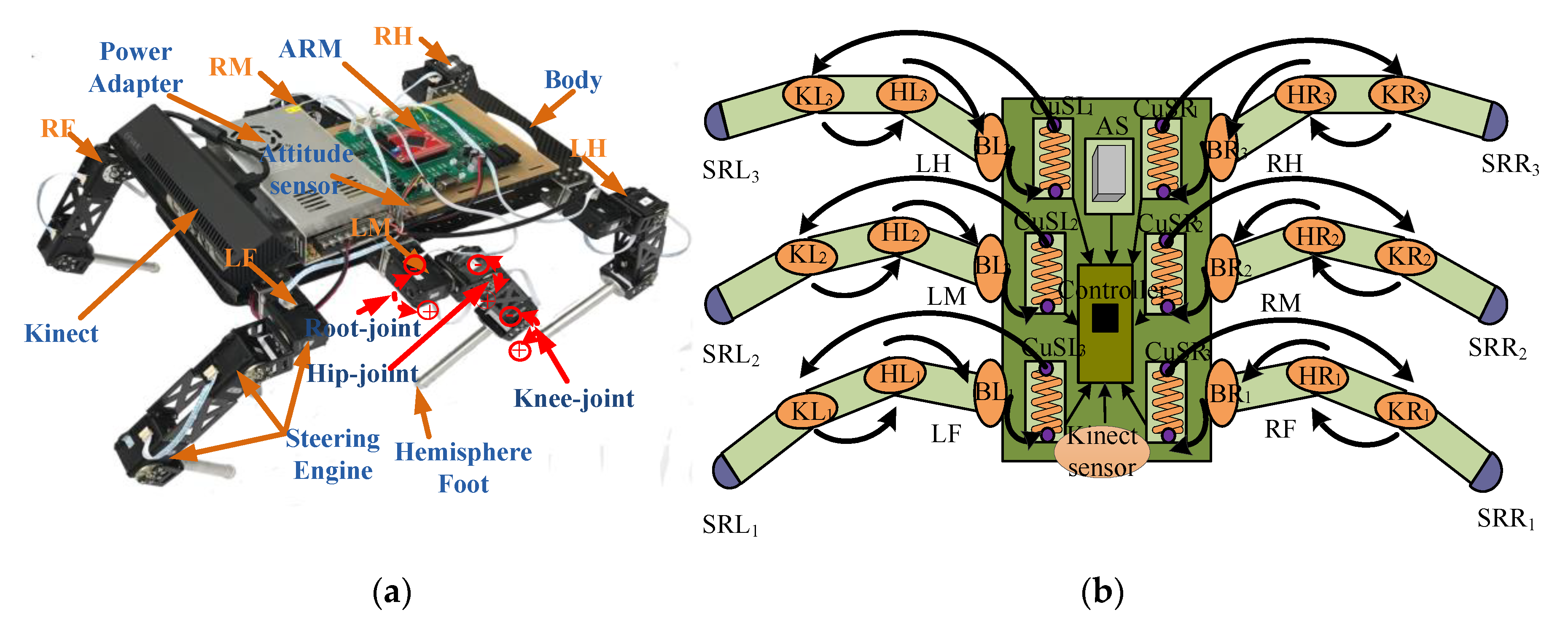
Figure 1. Architecture of robot: (a) hardware structure; (b) distribution of sensors. BLi, HLi, and KLi (BRi, HRi, and KRi), respectively, indicate base joint, hip joint, and knee joint of left (right) leg. LF, LM, and LH (RF, RM, and RH), respectively, indicate front leg, middle leg, and hind leg of left (right) side.
Applsci 09 01779 g001
Figure 2. Terrain classification system.
Applsci 09 01779 g002
Figure 3. Diagram of terrain classification system. BOW: bag-of-words; SVM: support vector machine.
Applsci 09 01779 g003
Figure 4. Different terrains and corresponding numbers of speeded up robust features (SURF) key points.
Applsci 09 01779 g004
Figure 5. Matching results of different algorithms: (a) SURF; (b) BRISK; (c) SURF-BRISK.
Applsci 09 01779 g005
Figure 6. Distributions of feature points in terrain with and without obstacles.
Applsci 09 01779 g006
Figure 7. ILI samples: (a) image sample; (b) local white; (c) local black; (d) local terrain.
Applsci 09 01779 g007
Figure 8. Distribution of terrain types: (a) single terrain; (b) mixed terrain.
Applsci 09 01779 g008
Figure 9. Segmentation result of mixed terrain images: (a) simple linear iterative cluster (SLIC) algorithm; (b) maximum super-pixel extraction; (c) filtering out smaller areas; (d) finding the boundary and fitting the line; (e) results.
Applsci 09 01779 g009
Figure 10. Number of feature points in segmented images.
Applsci 09 01779 g010
Figure 11. Number of feature points in spliced images.
Applsci 09 01779 g011
Figure 12. Recognition results: (a) terrain with obstacles; (b) mixed terrain.
Applsci 09 01779 g012
Figure 13. Gait transition.
Applsci 09 01779 g013
Table 1. Detection times of different descriptors. Brisk: binary robust invariant scalable keypoints.
Descriptor TypeDetection Time (ms)Matching Time (ms)
SURF8521251
BRISK12798
SURF-BRISK765142
Table 2. Classification results of first round and after image local infilling (ILI).
Images with Obstacle Applsci 09 01779 i001 Applsci 09 01779 i002 Applsci 09 01779 i003 Applsci 09 01779 i004 Applsci 09 01779 i005
First roundAsphaltAsphaltAsphaltAsphaltAsphalt
Actual terrainGrassGrassGrassGrassGravel
ILIWhiteAsphaltAsphaltTileTileTile
BlackAsphaltAsphaltAsphaltTileTile
TerrainGrassGrassGrassGrassGravel
Table 3. Image infilling and confidence scores.
Images Applsci 09 01779 i006 Applsci 09 01779 i007 Applsci 09 01779 i008 Applsci 09 01779 i009 Applsci 09 01779 i010
Actual terrainTileGrassTileGrassGrass
Output labelAsphaltTileAsphaltAsphaltSoil
R-ITileGrassTileGrassGrass
ScoresBeforeAfterBeforeAfterBeforeAfterBeforeAfterBeforeAfter
Sand10.079.5615.3614.5812.6410.4311.1912.4110.538.72
Grass8.428.0121.6528.0515.6813.0526.4337.4534.2345.18
Asphalt31.4115.6816.4715.1219.2915.6425.3714.5614.7610.63
Gravel14.5516.5615.8316.4515.6713.5414.3613.2211.78.35
Tile22.0136.0517.2614.6722.3631.7310.278.6818.2915.64
Soil13.5414.1413.4311.1314.3715.6212.3813.6910.511.48
Table 4. Gait transition algorithm.
  Initialize G∈[0.5 1]; SD∈{Dij = 0, j = 1, 2, … , 6; i = 1, 2, … , 2n}; B∈{0, 1}; n = 0; Ti∈{1, 2, …, 6}
    Repeat:
    (1) Collect terrain images: color, depth, and infrared;
    (2) Run the obstacle detection module and output B
         if B = 1 then
            Run image infilling processing I
            Jump to (2)
         else if B = 0 then
            continue
         end
    (3) Run the terrain classifier module and output SD
         for i = 1; i ≤ 2n; i++
            if max {Dij, (j = 1, 2, …, 6)} < 0.3 then
                n++
                Run image segmentation processing
                Run image infilling processing II
                Jump to repeat (3);
            Else if
                output the subscript j of max {Dij, (j = 1, 2, …, 6)};
                Ti = j
            end
         end
    (4) Output classification results and gait G
         for i = 1; i ≤ 2n–1; i++
            if Ti = 1 or 2 then G = 0.5
                else if Ti = 3 or 4 then G = 0.75
                else if Ti = 5 or 6 then G = 0.83
             end
         end
         T = T1,T2,T3, …, T2n–1
    (5) Run the robot
    Until: The robot is switched off.
  Note: G is the walking gait; typically, 0.5 for tripod gait, 0.75 for quadruped gait, and 0.83 for wave gait. SD is the confidence score; j refers to terrain type: 1 for asphalt, 2 for tile, 3 for soil, 4 for gravel, 5 for sand, 6 for grass; i is the serial number of images; B refers to the result of obstacle detection: B = 1 means there is an obstacle, B = 0 means no obstacle. Ti is the output label of the terrain classifier. Image infilling processing I represents the ILI module, and image infilling processing II represents the SPI module.
Table 5. Comparison of recent terrain classification methods.
Author or Method (Year)FeatureClassification MethodNumber of TerrainsFor Mixed Terrain?Application
Khan (2011) [8]SURF/DAISYSVM5NoVisual terrain classification
Zenker (2013) [11]SURF/SIFTSVM8NoEnergy-efficient gait
Filitchkin (2012) [17]SURFSVM6YesSelecting predetermined gaits
Lee (2011) [37]SURFANN5NoOff-road terrain classification for UGV
Ordonez (2013) [38]Characteristic frequency of leg currentPNN4NoRobot planning and motor control
Holder (2016) [39]Convolutional encoder–decoderCNN/SVM12YesReal-time road-scene understanding
Dallaire (2015) [40]Tactile dataMixture of Gaussians12NoGait switching
Manduchi (2005) [41]Color-basedMixture of Gaussians3NoRecognizing different terrains and obstacles
This paper (2017)SURF-BRISKSVM6YesAll kinds of outdoor robots