An Efficient Neural Network for Shape from Focus with Weight Passing Method

Abstract

In this paper, we suggest an efficient neural network model for shape from focus along with weight passing (WP) method. The neural network model is simplified by reducing the input data dimensions and eliminating the redundancies in the conventional model. It helps for decreasing computational complexity without compromising on accuracy. In order to increase the convergence rate and efficiency, WP method is suggested. It selects appropriate initial weights for the first pixel randomly from the neighborhood of the reference depth and it chooses the initial weights for the next pixel by passing the updated weights from the present pixel. WP method not only expedites the convergence rate, but also is effective in avoiding the local minimization problem. Moreover, this proposed method may also be applied to neural networks with diverse configurations for better depth maps. The proposed system is evaluated using image sequences of synthetic and real objects. Experimental results demonstrate that the proposed model is considerably efficient and is able to improve the convergence rate significantly while the accuracy is comparable with the existing systems.

1. Introduction

Among the variety of three-dimensional (3D) shape recovery techniques, shape from focus (SFF) is a passive optical method that infers 3D structure of an object from its image stack taken with different focus settings. During the last decade, SFF method has gained considerable attention due to its simplicity and economical computational cost and its considerable usage in computer vision and industrial applications such as 3D cameras, manufacture of thin-film-transistor liquid-crystal display (TFT-LCD) color filters, measurement of surface roughness, medical examination, microelectronics, focus variation for 3D surface [1,2,3,4,5,6,7,8]. In SFF, a sequence of images is captured through a single charge-coupled device (CCD) camera by translating object towards the camera in limited and small steps. Next, a focus measure is applied to measure the focus quality for each pixel in the sequence then an initial depth map is obtained by maximizing the focus measure in the direction of optical axes. Finally, an approximation or a machine learning method is applied to refine the initial depth estimate. Various approximation and machine learning-based methods have been suggested to extract and refine the object shape. The refinement process, generally, provides better depth maps as compared to the focus measure aggregation; however, these are computationally expensive.

Artificial neural network models have been successfully used to estimate optimal or near-optimal solutions of complex problems using a set of input-output data examples [9]. In case of SFF, however, exemplary data set is not available. In [10], SFF problem is defined as optimization of focus measure in terms of neural network weights over a three-dimensional focused image surface (FIS). An artificial neural network is trained to learn the shape of FIS (NN.FIS) in a small window by updating network weights in the direction of gradient of the focus measure. It yields considerably accurate depth estimates, but it suffers from high computational complexity and low convergence rate. The high complexity and slow convergence of the model are due to the large numbers of inputs and inappropriate initial weight. In NN.FIS, the inputs are taken by including the neighborhood frames that enlarge the size of weight vector. The initial weights are randomly set that can slow the convergence rate and lead to high computational cost. In addition, the accuracy is limited by the fact that the model may face local minimization problem.

In this paper, we propose a neural network over planar (NN.Planar) model for decreasing computational complexity. In order to increase the convergence rate and efficiency, weight passing (WP) is suggested. Our two contributions can be summarized as (1) a simplified neural network model is proposed that takes input and weight vector of smaller size; and (2) the WP method is proposed that selects proper initial weights for the first pixel randomly and it updates the initial weights for the next pixel efficiently by passing the updated weight from the present pixel. The proposed NN.Planar with WP method is not only efficient and simplified but also expedites the convergence rate and helps in avoiding the local minimization problem. Moreover, the proposed methods may also be applied to (NN.FIS) for better depth maps. The proposed method improves the convergence rate significantly and provides accurate depth maps. Experimental results demonstrate that the proposed model is significantly efficient while the accuracy is comparable with the conventional model.

2. Related Work

The goal of SFF is to detect the 3D depth of every point of an object from a camera lens. At first, an image sequence of the object is obtained by a single camera at different distances between lens and object. Principle of image sequence acquisition is illustrated in Figure 1. It shows an arrangement to estimate the shape of the object which is unknown body. The reference plane is the initial stage and the focused plane means a plane which is completely focused onto the sensor plane. The displacement of translational stage and the distance between the reference plane and the focused plane can be measured by experiment. Specifically, the translational stage is moved from reference plane in the direction of optical axes with a finite steps. At every step, an image is taken and a sequence of images at different step is obtained.

Focus measure plays an important role in SFF methods. In literature, several focus measure operators have been proposed in the spatial and the frequency domains. The performance of the focus measure operator depends on several factors including local window size, imaging device specifications, illumination conditions and complexity of object shape. The effect of window sizes on depth map recovery is studied by Malik and Choi [11] and concluded that a larger window may distort the object shape while a smaller window size may not be able to suppress noise properly. Recently, a comprehensive study by Pertuz et al. [12] demonstrates the effects of various factors on 3D shape recovery using various focus measures. The study also serves a good reference for focus measure operators in various domains. In noise free environment, second derivative-based focus measure Sum-Modified-Laplacian (SML) [13] performs better whereas in noisy environment Gray-Level-Variance (GLV) [12] provides better depth maps.

Once focus values for all pixels in the sequence are computed, various approximation and machine learning-based methods have been suggested to extract and refine the object shape. The simplest approximation method used in earlier works is to replace the central pixel with aggregated focus measures in a small window. Then depth map is obtained by maximizing focus measure along the optical direction from the refined focus volume [11]. The aggregation of focus measures is efficient to compute but it may not provide accurate depth map. On the other hand, several optimization and machine learning-based approaches have been proposed for better 3D shapes [10,14,15,16,17]. Ahmad and Choi [14] proposed the usage of dynamic programming to obtain optimal focus measure. It is difficult to apply dynamic programming on 3D volume directly so authors applied it on two-dimensional (2D) slices that has decreased its effectiveness. In [17], authors proposed maximum a posteriori (MAP)-based framework for SFF that utilizes local learning process to build a consistency model directly from image focus volume. It improves accuracy and obtains consistent depth maps, but it needs additional computations in local learning process. Recently, in [15], authors suggested anisotropic diffusion process with regularization to obtain better depth map. The above-mentioned approaches provide better depth maps as compared to the focus measure aggregation however, these are also computationally expensive.

In machine learning-based methods, one of the important issues is to develop proper representations for complex data. In literature, various dimensionality reduction models are proposed to reduce the complexity. In [18], authors suggested global geometric framework to discover the nonlinear degrees of freedom that consists of natural multivariate data. It improves efficiency for computing a globally optimal solution than the conventional techniques such as principal component analysis (PCA) [19] and multidimensional scaling (MDS) [20]. In [21], authors developed predictors based on support vector machine (SVM) for feature extraction. They applied various dimensionality reduction models including PCA and independent component analysis (ICA). The results of this study show that SVM by feature extraction using PCA performs better than SVM without using PCA or ICA. In [22], an unsupervised learning algorithm, called locally linear embedding (LLE), is proposed. It maps its inputs into a single global coordinate without local minimization problem. In [23], authors proposed a geometrically motivated algorithm for nonlinear dimensionality reduction having locality-preserving properties. Another alternative research suggests pre-process the input data before feature extraction. In [24], authors presented an application of deep networks to learn features over multiple modalities using an extension of restricted Boltzmann machines (RBM). The multiple features provide considerably better models and reduce dimensionality. Similarly, in [25], authors proposed a method to estimate the motion based on virtual character. The motion features are pre-processed using RBM. In [26], authors proposed a data-processing pipeline based on sparse feature learning using RBM.

3. Neural Network for SFF

3.1. Neural Network Model over FIS

The neural network model over FIS (NN.FIS) proposed in [10] employs a three layers neural network model as shown in Figure 2. The input layer consists of three linear neurons and hidden layer contains sigmoidal neurons with an additional linear neuron. Whereas the third layer is composed of one sigmoidal neuron and it provides output in the range [0, 1].

At an iteration $\left(n\right)$, the local depth map $z_{(x,y)}^{\left(n\right)}(j,k)$ for a small window of size $M\times M$ centered at global index $(x,y)$ is described as:

$$z_{(x,y)}^{\left(n\right)}(j,k)=\varphi \left({\left({\mathbf{v}}^{\left(n\right)}\right)}^T·\varphi \left({\mathbf{U}}^{\left(n\right)}·\mathbf{i}\right)+w_b^{\left(n\right)}\right)$$

(1)

where $(j,k)$ is spatial representation of the local index values in the window, ${\mathbf{U}}^{\left(n\right)}\in {\mathbb{R}}^{H\times 3}$ and ${\mathbf{v}}^{\left(n\right)}\in {\mathbb{R}}^H$ are the network weight matrices between the layers, H is the number of sigmoidal neurons. $w_b^{\left(n\right)}$ represents the bias, $\mathbf{i}={\left[jk1\right]}^T$ is the input vector, ${(·)}^T$ indicates transpose function of the matrix function, and $\varphi (·)$ is the sigmoidal function.

The focus measure F is calculated from $z_{(x,y)}^{\left(n\right)}(j,k)$ by GLV as follows:

$$F=\sum _{\begin{array}{c}-m\le j\le m\\ -m\le k\le m\end{array}}{\left[I\left(x+j,y+k,z_{(x,y)}^{\left(n\right)}(j,k)\right)-\mu \right]}^2$$

(2)

where $I\left(x+j,y+k,z_{(x,y)}^{\left(n\right)}(j,k)\right)$ is the gray level at $(x+j,y+k)$ in the frame number $z_{(x,y)}^{\left(n\right)}(j,k)$, $m=(M-1)/2$ the local index bound, and $\mu$ represents the average gray level of the pixels on the window surface defined by $z_{(x,y)}^{\left(n\right)}(j,k)$ as:

$$\mu =\frac{1}{M^2}\sum _{\begin{array}{c}-m\le j\le m\\ -m\le k\le m\end{array}}I\left(x+j,y+k,z_{(x,y)}^{\left(n\right)}(j,k)\right)$$

(3)

It is important to note that F and $\mu$ are the functions of $z_{(x,y)}^{\left(n\right)}(j,k)$. Accordingly, these functions not only depend on global index $(x,y)$ but also depend on local index $(j,k)$. It means, they can only be calculated during the network learning. Consequently, the complexity rises sharply.

Generally, feedforward neural networks are utilized for learning an input-output relationship from the given example data set. In case of neural networks for SFF, there is no such an example data set available. Therefore, it is a distinctive application of neural networks where a focus measure, which is role of a performance function, is to be optimized. The network weights are updated according to the gradient decent rule as follows:

$$\begin{array}{ccc}\hfill \Delta {\mathbf{W}}^{\left(n\right)}& =\hfill & \hfill -\beta \left(\frac{\partial E}{\partial {\mathbf{W}}^{\left(n\right)}}\right)\\ & =\hfill & \hfill \beta \left(\frac{\partial F}{\partial {\mathbf{W}}^{\left(n\right)}}\right)\end{array}$$

(4)

where $\Delta {\mathbf{W}}^{\left(n\right)}$ means the net change of the weight matrix ${\mathbf{W}}^{\left(n\right)}$, which includes ${\mathbf{U}}^{\left(n\right)}$, ${\mathbf{v}}^{\left(n\right)}$, and $w_b^{\left(n\right)}$, whereas $\beta$ is the learning rate. In addition, $E=-F$ is the minimization criterion. At each iteration weights are updated and consequently $z_{(x,y)}^{\left(n\right)}(j,k)$ are also updated. At the last iteration $\left(N\right)$, the final depth at $(x,y)$ is obtained as:

$$d(x,y)=z_{(x,y)}^{\left(N\right)}(0,0)$$

(5)

and the final restored depth map from the NN.FIS model is represented as:

$$F_{NN.FIS}=\left\{d(x,y)|x\in [1,\dots ,I_W],y\in [1,\dots ,I_H]\right\}$$

(6)

where $I_W$ and $I_H$ are the width and the height of each image in the sequence, respectively.

3.2. Proposed Model

In NN.FIS a focus value is computed from a current frame ($z_{(x,y)}^{\left(n\right)}(0,0)$) and its neighboring frames ($z_{(x,y)}^{\left(n\right)}(j,k)$) that increases the size of the weight matrix $\mathbf{W}$ and over all complexity for shape recovery become high. We have observed through the experiments that the focus measure computed from the current frame not only provides smaller weight matrix but also reduces the time complexity remarkably without compromising on accuracy. Figure 3 shows the proposed neural network model over planar surface (NN.Planar) for shape from focus. In SFF, a planar surface is considered in 3D space, however, in this paper “planar” means only on the same frame i.e., 2D surface. From the figure, it can be observed that the number of neurons at the input layer are decreased from three to one. In the NN.Planar, the depth $z_{(x,y)}^{\left(n\right)}$ at iteration $\left(n\right)$ for the central pixel $(x,y)$ of the window can be expressed as:

$$z_{(x,y)}^{\left(n\right)}=\varphi \left({\left({\mathbf{v}}^{\left(n\right)}\right)}^T·\varphi \left({\mathbf{u}}^{\left(n\right)}\right)+w_b^{\left(n\right)}\right)$$

(7)

where ${\mathbf{u}}^{\left(n\right)}\in {\mathbb{R}}^H$, ${\mathbf{v}}^{\left(n\right)}\in {\mathbb{R}}^H$, and $w_b^{\left(n\right)}\in \mathbb{R}$, and $\varphi (·)$ is sigmoidal function defined as:

$$\varphi \left(\eta \right)=\frac{1}{1+e^{-\eta }}$$

(8)

where $\eta$ is a dummy variable.

Accordingly, in the NN.Planar, the focus measure F is calculated as

$$F=\sum _{\begin{array}{c}-m\le j\le m\\ -m\le k\le m\end{array}}{\left[I\left(x+j,y+k,z_{(x,y)}^{\left(n\right)}\right)-\mu \right]}^2$$

(9)

where $I\left(x+j,y+k,z_{(x,y)}^{\left(n\right)}\right)$ is the gray level at the pixel position of $(x+j,y+k)$ in the frame number $z_{(x,y)}^{\left(n\right)}$, and $\mu$ represents the mean of gray levels within the window and it is expressed as

$$\mu =\frac{1}{M^2}\sum _{\begin{array}{c}-m\le j\le m\\ -m\le k\le m\end{array}}I\left(x+j,y+k,z_{(x,y)}^{\left(n\right)}\right)$$

(10)

In order to update weights, we use gradient descent rule. Note that, in NN.Planar, a scalar depth is computed instead of a matrix (as in the case of NN.FIS model) therefore the computation of gradient becomes simplified. Moreover, it becomes more efficient due to the reduced dimensions of ${\mathbf{u}}^{\left(n\right)}$. By using chain rule, Equation (4) can be written as

$$\begin{array}{ccc}\hfill \Delta {\mathbf{W}}^{\left(n\right)}& =& \beta \left(\frac{\partial F}{\partial {\mathbf{W}}^{\left(n\right)}}\right)\hfill \\ & =& \beta \left(\frac{\partial F}{\partial z_{(x,y)}^{\left(n\right)}}\right)·\left(\frac{\partial z_{(x,y)}^{\left(n\right)}}{\partial {\mathbf{W}}^{\left(n\right)}}\right)\hfill \\ & =& 2\beta \sum _{\begin{array}{c}-m\le j\le m\\ -m\le k\le m\end{array}}\left[I\left(x+j,y+k,z_{(x,y)}^{\left(n\right)}\right)-\mu \right]\hfill \\ & & ·\left(\frac{\partial \left[I\left(x+j,y+k,z_{(x,y)}^{\left(n\right)}\right)-\mu \right]}{\partial z_{(x,y)}^{\left(n\right)}}\right)\hfill \\ & & ·\left(\frac{\partial z_{(x,y)}^{\left(n\right)}}{\partial {\mathbf{W}}^{\left(n\right)}}\right)\hfill \end{array}$$

(11)

Here $\mu$ is constant, thus Equation (11) can be written as

$$\begin{array}{ccc}\hfill \Delta {\mathbf{W}}^{\left(n\right)}& =& 2\beta \sum _{\begin{array}{c}-m\le j\le m\\ -m\le k\le m\end{array}}\left[I\left(x+j,y+k,z_{(x,y)}^{\left(n\right)}\right)-\mu \right]\hfill \\ & & ·\left(\frac{\partial I\left(x+j,y+k,z_{(x,y)}^{\left(n\right)}\right)}{\partial z_{(x,y)}^{\left(n\right)}}\right)\hfill \\ & & ·\left(\frac{\partial z_{(x,y)}^{\left(n\right)}}{\partial {\mathbf{W}}^{\left(n\right)}}\right)\hfill \end{array}$$

(12)

where $I\left(x+j,y+k,z_{(x,y)}^{\left(n\right)}\right)$ represents gray level values in the window, and the term $\left(\partial I\left(x+j,y+k,z_{(x,y)}^{\left(n\right)}\right)/\partial z_{(x,y)}^{\left(n\right)}\right)$ is the derivative of the image intensity of the window surface with respect to the image frame number $z_{(x,y)}^{\left(n\right)}$. The derivative can be implemented as

$$\frac{\partial I\left(x+j,y+k,z_{(x,y)}^{\left(n\right)}\right)}{\partial z_{(x,y)}^{\left(n\right)}}=\frac{I_{+}-I_{-}}{2h}$$

(13)

where h is a step size, $I_{+}=I\left(x+j,y+k,z_{(x,y)}^{\left(n\right)}+h\right)$, and $I_{-}=I\left(x+j,y+k,z_{(x,y)}^{\left(n\right)}-h\right)$. The remaining term $\left(\partial z_{(x,y)}^{\left(n\right)}/\partial {\mathbf{W}}^{\left(n\right)}\right)$, which is surface gradient, can be acquired using backpropagation algorithm [9]. Here, the weight ${\mathbf{W}}^{\left(n\right)}$ includes ${\mathbf{u}}^{\left(n\right)}$, ${\mathbf{v}}^{\left(n\right)}$, and $w_b^{\left(n\right)}$, and their derivatives are expressed as

$$\begin{array}{ccc}\hfill \frac{\partial z_{(x,y)}^{\left(n\right)}}{\partial {\mathbf{u}}^{\left(n\right)}}& =& z_{(x,y)}^{\left(n\right)}·\left(1-z_{(x,y)}^{\left(n\right)}\right)·{\mathbf{v}}^{\left(n\right)}\hfill \\ & & \ast \left[\varphi \left({\mathbf{u}}^{\left(n\right)}\right)\ast \left(1-\varphi \left({\mathbf{u}}^{\left(n\right)}\right)\right)\right]\hfill \end{array}$$

(14)

$$\begin{array}{ccc}\hfill \frac{\partial z_{(x,y)}^{\left(n\right)}}{\partial {\mathbf{v}}^{\left(n\right)}}& =& z_{(x,y)}^{\left(n\right)}·\left(1-z_{(x,y)}^{\left(n\right)}\right)·\varphi \left({\mathbf{u}}^{\left(n\right)}\right)\hfill \end{array}$$

(15)

$$\begin{array}{ccc}\hfill \frac{\partial z_{(x,y)}^{\left(n\right)}}{\partial w_b^{\left(n\right)}}& =& z_{(x,y)}^{\left(n\right)}·\left(1-z_{(x,y)}^{\left(n\right)}\right)\hfill \end{array}$$

(16)

where ∗ denotes the element-by-element multiplication of vectors. Using Equations (12)–(16), the weights are updated as

$$\begin{array}{ccc}\hfill {\mathbf{u}}^{(n+1)}& =& {\mathbf{u}}^{\left(n\right)}+\beta ·G^{\left(n\right)}·\frac{\partial z_{(x,y)}^{\left(n\right)}}{\partial {\mathbf{u}}^{\left(n\right)}}\hfill \end{array}$$

(17)

$$\begin{array}{ccc}\hfill {\mathbf{v}}^{(n+1)}& =& {\mathbf{v}}^{\left(n\right)}+\beta ·G^{\left(n\right)}·\frac{\partial z_{(x,y)}^{\left(n\right)}}{\partial {\mathbf{v}}^{\left(n\right)}}\hfill \end{array}$$

(18)

$$\begin{array}{ccc}\hfill w_b^{(n+1)}& =& w_b^{\left(n\right)}+\beta ·G^{\left(n\right)}·\frac{\partial z_{(x,y)}^{\left(n\right)}}{\partial w_b^{\left(n\right)}}\hfill \end{array}$$

(19)

where $G^{\left(n\right)}$ is represented as

$$\begin{array}{ccc}\hfill G^{\left(n\right)}& =& 2\sum _{\begin{array}{c}-m\le j\le m\\ -m\le k\le m\end{array}}\left[I\left(x+j,y+k,z_{(x,y)}^{\left(n\right)}\right)-\mu \right]\hfill \\ & & ·\left(\frac{\partial I\left(x+j,y+k,z_{(x,y)}^{\left(n\right)}\right)}{\partial z_{(x,y)}^{\left(n\right)}}\right)\hfill \end{array}$$

(20)

Note that $G^{\left(n\right)}$ is pre-calculable value before network learning. Essentially, it is dependent on global indexes $(x,y)$ and the network output $z_{(x,y)}^{\left(n\right)}$, and thus it is dependent on the network learning iteration $\left(n\right)$. However, a possible set of $G^{\left(n\right)}$ can be calculated in advance of network learning, because the number of elements of the possible set is same to the total frame number $I_D$ of image sequence. Therefore, it gives additional time efficiency. After updating ${\mathbf{W}}^{(n+1)}$ as Equations (17)–(19), the present iteration $\left(n\right)$ is ended, and it follows the next iteration $(n+1)$. In this manner, all $z_{(x,y)}^{\left(n\right)}$ at each iteration are updated and the final depth map for $(x,y)$ can be acquired as

$$d(x,y)=z_{(x,y)}^{\left(N\right)}$$

(21)

And the final depth map of NN.Planar at all points is described as

$$F_{NN.Planar}=\left\{d(x,y)|x\in [1,\dots ,I_W],y\in [1,\dots ,I_H]\right\}$$

(22)

The proposed NN.Planar looks an instance of the NN.FIS as proposed in [10]. Consider a particular instance of NN.FIS by restricting the input vector $\mathbf{i}={\left[jk1\right]}^T$ with $j=0$, $k=0$. In this case, it needs to update not only weights connected from the bias 1 but also weights connected from j and k. Weights update, related to j and k, for focus measure over a planar surface is redundant in NN.FIS. Therefore, the proposed NN.Planar is not an instance of the NN.FIS. Moreover, in the NN.FIS, neighboring points are taken into account to compute the complex shape of FIS. Whereas the proposed NN.Planar is based on the assumption of planar surface. In other words, the surface within the local window is assumed to be a planar surface. It may seem to be similar to the piece-wise constant approximation. However, it is not constant as it is modelled through the functions (7) and (9) to provide accurate depth.

4. Initial Weight Setting

In neural network-based SFF methods, initial network weights play important role in acquiring accurate depth map, network convergence, and time complexity. If the initial weights for a pixel are not set properly, more likely an incorrect initial depth map is obtained. Consequently, the convergence of the network is affected by these inaccuracies in depth map and improper initial weights. Therefore, in NN.FIS and NN.Planar networks, it is important to select suitable initial weights for rapid convergence of the networks and for obtaining accurate final depth maps.

Usually, initial weights are selected randomly. However, random weights may not provide rapid convergence and accurate depth map. In order to overcome these problems, we propose WP method for setting proper initial weights. Using WP method, the network converges rapidly, provides more precise depth map and reduces the time complexity. Furthermore, it helps in avoiding the local minimization problem effectively. Before explaining the proposed WP method, it would be worthy to describe the random setting (RS).

4.1. RS Initial Weight Setting Method

In [10], the initial weights for each pixel are determined randomly. If the initial depth map significantly deviate from the desired depth map generated from the initial weight, it may lead to local minimization problem and network may fail in obtaining a precise depth map. Furthermore, this method may lead to slow convergence of the network as it needs larger numbers of iterations for 3D shape learning. In other words, it fails to estimate a depth precisely with a high probability if the initial weights for a pixel are determined randomly. Therefore, in [27], initial weights are taken randomly around a reference depth map $z_r(x,y)$ to complement the problem. In this paper, we call it RS method. The RS method is summarized in Algorithm 1. At first, a test set of initial weights ($\mathbf{u}$, $\mathbf{v}$, and $w_b$) are randomly generated in the range $[0,1]$. Next, $z_{(x,y)}^{\left(1\right)}$ is calculated using Equation (7). Then, the distance between initial depth $z_{(x,y)}^{\left(1\right)}$ and the reference depth $z_r(x,y)$ is compared with the threshold $T_1$. If the distance is less than or equal to $T_1$, the test set of initial weights are regarded as the proper initial weights for $(x,y)$ and are used for further computation of (${\mathbf{u}}^{\left(1\right)}$, ${\mathbf{v}}^{\left(1\right)}$, and $w_b^{\left(1\right)}$). On the other side, if the distance is greater than to $T_1$ then again initial weights are generated randomly and the distance is compared with $T_1$. This process is repeated for a certain times; say $R=1000$. If the proper weights are not found within R iterations then an inaccurate depth for $(x,y)$ may be computed. Once weights are obtained, the depth for $(x,y)$ is estimated through NN.Planar (or NN.FIS) model using Equations (7)–(21) (or Equations (1)–(5)) with ${\mathbf{u}}^{\left(1\right)}$, ${\mathbf{v}}^{\left(1\right)}$, and $w_b^{\left(1\right)}$. In this way, the entire depth map is obtained by computing depth for all pixel positions.

In summary, this method has two main problems: (1) the time complexity is significantly increased by determining the initial weights for every pixel position; and (2) If the initial depth map is close to the reference depth map, RS method may avoid the local minimization problem and can provide reasonable initial weights however, when the reference depth map is near to the minimum or maximum value of depth range, it is hard to get proper initial weights and accurate depth map. This phenomena is highlighted in Figure 4. It shows the histogram of $z_{(x,y)}^{\left(1\right)}$ and represents the distribution of numerical data of $z_{(x,y)}^{\left(1\right)}$ from 10,000 trials of Equation (7) by using random weights. From Figure 4, we can find that the frequency is very low near to the minimum or maximum depth values. Consequently, it is hard to meet the requirements of $|z_{(x,y)}^{\left(1\right)}-z_r(x,y)|\le T_1$ within R trials, and thus it is hard to set the proper initial weights in RS method. For example, if $z_r(x,y)=0.05$ and $T_1=0.02$, and then $z_{(x,y)}^{\left(1\right)}$ should be in $[0.03,0.07]$. However, there is low probability that $z_{(x,y)}^{\left(1\right)}$ be within $[0.03,0.07]$ after R trials, thus there is high probability of not setting proper initial weights.

Algorithm 1. Random Setting method.

1: procedureRandom Setting 2:       for $x=1$ to $I_W$ do 3:            for $y=1$ to $I_H$ do 4:               for $i=1$ to R do 5:                    Generate initial weights $\mathbf{u},\mathbf{v},w_b$ randomly. 6:                    $z_{(x,y)}^{\left(1\right)}\leftarrow \varphi \left({\left(\mathbf{v}\right)}^T·\varphi \left(\mathbf{u}\right)+w_b\right)$ 7:                    if $|z_{(x,y)}^{\left(1\right)}-z_r(x,y)|\le T_1$ then 8:                         ${\mathbf{u}}^{\left(1\right)}\leftarrow \mathbf{u}$ 9:                         ${\mathbf{v}}^{\left(1\right)}\leftarrow \mathbf{v}$ 10:                         $w_b^{\left(1\right)}\leftarrow w_b$ 11:                         break 12:                    end if 13:               end for 14:               $d(x,y)\leftarrow$ estimated depth at $(x,y)$ by using Equations (7)–(21) (or Equations (1)–(5)) 15:            end for 16:       end for 17: end procedure

4.2. Proposed WP Method

Figure 4 highlights the distribution of initial depth $z_i$. From the figure, it can be observed that the initial depth values near the extremities may affect the procedure of choosing the proper initial weights. Particularly, the RS method may produce an erroneous initial depth values near the extremities as theses depth values may considerably deviate from the precise depth. This phenomena can also be understandable as there is high probability that $G^{\left(1\right)}$ may be near to zero at these condition. Therefore, weights will become stagnant as this fact can be observed from Equations (17)–(19). It can be concluded that the initial depth needs to be close to the precise depth for avoiding local minimization problem. Therefore, WP method is proposed to relieve the local minimization regardless of a depth range of a reference depth map.

The proposed WP method is described in Algorithm 2. In the proposed algorithm, in first step, a 2-dimensional reference depth map $z_r(x,y)$ patch is converted into 1-dimensional reference depth vector $z_r\left(s\right)$. In the second step, a new vector ${\widehat{z}}_r\left(t\right)$ is obtained by sorting $z_r\left(s\right)$ with respect to depth in ascending order. In third step, an index vector $\widehat{s}\left(t\right)$ is acquired by rearranging the indices of $z_r\left(s\right)$ corresponding to the depth at ${\widehat{z}}_r\left(t\right)$. In fourth step, 2-dimentional indices $(\widehat{x}\left(t\right),\widehat{y}\left(t\right))$ are acquired by rearranging the index of 2-dimentional patch $z_r(x,y)$ corresponding to the depth at ${\widehat{z}}_r\left(t\right)$. In order to describe these four steps, an example is shown in Figure 5. In fifth step, the proper initial weights for the first pixel $z_r(\widehat{x}\left(1\right),\widehat{y}\left(1\right))$ are obtained by comparing the initial depth with the reference depth. In sixth step, a depth for $(\widehat{x}\left(t\right),\widehat{y}\left(t\right))$ is estimated through the NN.Planar model as using Equations (7)–(21) with ${\mathbf{u}}^{\left(1\right)}$, ${\mathbf{v}}^{\left(1\right)}$, and ${\mathbf{w}}_{\mathbf{b}}^{\left(1\right)}$. In next step, initial weights for the next pixel are set by passing updated weights from the present pixel. In this way, the entire depth map is estimated by repeating the steps 6–7 for all pixel positions.

Algorithm 2. Weight Passing method.

1: procedureWeight Passing 2:       $z_r\left(s\right)\leftarrow$$z_r(x,y)$  ▹ Change 2-dimensional $z_r(x,y)$ into 1-dimensional vector form $z_r\left(s\right)$ 3:       ${\widehat{z}}_r\left(t\right)\leftarrow$ sorted $z_r\left(s\right)$ into depth order 4:       $\widehat{s}\left(t\right)\leftarrow$ rearranged the index of $z_r\left(s\right)$ corresponding to the depth of ${\widehat{z}}_r\left(t\right)$ 5:       $(\widehat{x}\left(t\right),\widehat{y}\left(t\right))\leftarrow$ rearranged the index of $z_r(x,y)$ corresponding to the depth of ${\widehat{z}}_r\left(t\right)$ 6:       for $i=1$ to R do 7:         Generate initial weights $\mathbf{u},\mathbf{v},w_b$ randomly. 8:         $z_{(x,y)}^{\left(1\right)}\leftarrow \varphi \left({\left(\mathbf{v}\right)}^T·\varphi \left(\mathbf{u}\right)+w_b\right)$ 9:         if $|z_{(x,y)}^{\left(1\right)}-z_r(\widehat{x}\left(1\right),\widehat{y}\left(1\right))|\le T_1$ then 10:           ${\mathbf{u}}^{\left(1\right)}\leftarrow \mathbf{u}$ 11:           ${\mathbf{v}}^{\left(1\right)}\leftarrow \mathbf{v}$ 12:           $w_b^{\left(1\right)}\leftarrow w_b$ 13:           break 14:         end if 15:       end for 16:       for $t=1$ to $(I_W·I_H)$ do 17:         $d(\widehat{x}\left(t\right),\widehat{y}\left(t\right))\leftarrow$ estimated depth at $(\widehat{x}\left(t\right),\widehat{y}\left(t\right))$ pixel position by using Equations (7)–(21) (or Equations (1)–(5)) 18:         ${\mathbf{u}}^{\left(1\right)}\leftarrow$ updated weight ${\mathbf{u}}^{\left(N\right)}$ 19:         ${\mathbf{v}}^{\left(1\right)}\leftarrow$ updated weight ${\mathbf{v}}^{\left(N\right)}$ 20:         $w_b^{\left(1\right)}\leftarrow$ updated weight $w_b^{\left(N\right)}$ 21:       end for 22: end procedure

Note that the initial depth of $(\widehat{x}(i+1),\widehat{y}(i+1))$ is close to $d(\widehat{x}\left(i\right),\widehat{y}\left(i\right))$, because ${\mathbf{W}}^{\left(1\right)}$ for $(\widehat{x}(i+1),\widehat{y}(i+1))$ is allocated from ${\mathbf{W}}^{\left(N\right)}$ for $(\widehat{x}\left(i\right),\widehat{y}\left(i\right))$. In addition, there is high probability that the resultant depths for $d(\widehat{x}(i+1),\widehat{y}(i+1))$ and $d(\widehat{x}\left(i\right),\widehat{y}\left(i\right))$ may be very close to each other. Accordingly, $z_i$ satisfies the condition $|z_{(x,y)}^{\left(1\right)}-z_r(\widehat{x}\left(i\right),\widehat{y}\left(i\right))|\le T_1$ when $i\ge 2$. In summary, WP is advantageous in (1) reducing the chances of local minimization problem; (2) decreasing the total numbers of iterations for the stable solution; and (3) decreasing computational complexity for setting initial weights for all pixels.

5. Experiments

5.1. Experimental Setup

The performance of the proposed system consisting of NN.Planar model, WP initial weight setting method is evaluated using image sequences of synthetic and real objects. Synthetic objects plane, sinusoidal, cone, and wave are virtually created by simulation tool. For each object, synthetic image sequence is generated by using a defocus simulation tool box [28] with varying focus settings. Each synthetic image in the sequences is resultant of convolution of actual texture image and Point Spread Function (PSF). Thus, in the synthetic image sequence, the Gaussian function is taken as PSF, camera parameters and the true depth map of the synthetic object are used. For more details, refer to [12,29]. Image sequences for each synthetic object consists of 80 images (or frames) each with size $360\times 360$ pixels.

Figure 6a represents sample frames from image sequences of plane, sinusoidal, cone, and wave objects. From the figure, we can observe that some parts of the objects are well focused and others are out of focus with a degree of blur. And for evaluating the proposed algorithms in real world, we have performed experiments using real objects of real cone, engraved letter I, coin, and TFT-LCD color filter. An image sequence from real cone is obtained by using a CCD camera system with varying focus levels [3], and it consists of 97 images of 200 × 200 pixels. Other image sequences from microscopic objects of engraved letter I, coin, and TFT-LCD color filter are acquired by using a microscopic control system [2]. In the case of coin object, the image sequence consists of 68 frames of 300 × 300 pixels. And each image sequence from engraved letter I and TFT-LCD color filter consists of 60 images of 300 × 300 pixels. Sample frames from each image sequence are represented in Figure 6b.

In order to produce comparative analysis, first, depth maps have been obtained from image sequences by applying conventional methods and the proposed method. Then, the resultant depth maps are compared qualitatively and quantitatively. We performed experiments for networks NN.FIS and NN.Planar with combinations of RS initial weight setting method [10] and WP initial weight setting method. In the experiments, the numbers of hidden layer H, the total iteration number T, the window size $M\times M$ are set as 20, 50, $7\times 7$, respectively. Moreover, the learning rate $\beta$s: $19.92$, $2.35$, $6.15$, $7.23$, and $1.25$ are taken for synthetic objects, real cone, engraved letter I, coin, and TFT-LCD color filter, respectively. There is not any specific method to determine the size of the hidden layer H. If H is too large it suffers from expensive computation. On the other hand, if H is too small the network may not provide desired results. Therefore, H is determined empirically through experiments.

5.2. Quantitative Analysis

In order to evaluate the performance of the proposed system quantitatively, two quantitative metrics: Root-Mean-Square-Error (RMSE) and correlation (Corr). In the case of experiments for synthetic objects, it is possible to calculate RMSE and correlation as their true depth maps are available. Whereas it is impracticable to compute RMSE and correlation metrics for real objects as there true depth maps are not available. RMSE measures the distortion between the true depth map and the estimated depth map. It can be calculated as:

$$\mathrm{RMSE}=\sqrt{\frac{1}{I_W·I_H}\sum _{\begin{array}{c}1\le x\le I_W\\ 1\le y\le I_H\end{array}}{(z_t(x,y)-z_e(x,y))}^2}$$

(23)

where $z_t(x,y)$ and $z_e(x,y)$ are the true depth map and the estimated depth map respectively, $I_W$ and $I_H$ are the width and the height of the true and the estimated depth maps. correlation measures the similarity between the true depth map and the estimated depth map. It can be calculated as follows:

$$\mathrm{Corr}=\frac{{\sum }_{\begin{array}{c}1\le x\le I_W\\ 1\le y\le I_H\end{array}}(z_t(x,y)-\overline{z_t(x,y)})(z_e(x,y)-\overline{z_e(x,y)})}{{\sum }_{\begin{array}{c}1\le x\le I_W\\ 1\le y\le I_H\end{array}}{(z_t(x,y)-\overline{z_t(x,y)})}^2{(z_e(x,y)-\overline{z_e(x,y)})}^2}$$

(24)

where $\overline{z_t(x,y)}$ and $\overline{z_e(x,y)}$ are the mean of the true and the estimated depth map, respectively.

The performance comparison between conventional and proposed methods in terms of RMSE and correlation is shown in

Table 1. Performance Comparison for Various SFF methods using Various Synthetic Objects.

Object	SML	GLV	FIS with RS	Planar with RS	FIS with WP	Planar with WP
	RMSE (Corr)	RMSE (Corr)	RMSE (Corr)	RMSE (Corr)	RMSE (Corr)	RMSE (Corr)
Plane	4.589 (0.970)	3.805 (0.979)	4.196 (0.972)	4.073 (0.974)	3.217 0.985)	3.215 (0.985)
Sinusoidal	4.649 (0.978)	3.782 (0.985)	4.630 (0.977)	4.505 (0.978)	3.092 (0.990)	3.128 (0.990)
Cone	8.548 (0.957)	8.462 (0.971)	8.567 (0.967)	8.503 (0.970)	8.402 (0.978)	8.395 (0.978)
Wave	2.824 (0.979)	2.004 (0.989)	2.581 (0.981)	2.366 (0.984)	1.644 (0.992)	1.661 (0.992)

. The quantitative measures are calculated by using estimated depth maps through SML, GLV, NN.FIS with RS, NN.Planar with RS, NN.FIS with WP, and NN.Planar with WP. From Table 1, two meaningful results are (1) The performance is similar to each other between NN.FIS and NN.Planar with same initial weight setting method (NN.FIS with RS vs. NN.Planar with RS or NN.FIS with WP vs. NN.Planar with WP); and (2) the proposed WP generates more accurate estimated depth map than RS initial weight setting method (NN.FIS with RS vs. NN.FIS with WP or NN.Planar with RS vs. NN.Planar with WP). In the same manner,

Table 2. Experiment Time for Various SFF methods using Various Synthetic Objects.

Object	SML	GLV	FIS with RS	Planar with RS	FIS with WP	Planar with WP
Plane	17.8	24.6	15,347.3	2837.5	12,377.9	130.9
Sinusoidal	17.9	24.6	18,169.5	5336.5	12,504.5	129.9
Cone	17.8	24.8	13,183.0	928.4	12,922.5	135.9
Wave	17.8	24.6	13,829.0	977.9	12,595.6	130.4

shows the experiment time for various SFF methods using various synthetic objects. There are also two notable results (1) NN.Planar model is faster than NN.FIS model with same initial weight setting method; and (2) WP is faster than RS method. Specifically, NN.Planar with WP is about 90 times faster than NN.FIS with WP, and NN.Planar with WP is about 100 to 140 times faster than NN.FIS with RS. Note that RS method gains additional complexity because of setting initial weights for all pixels of an object. In addition, the additional complexity varies considerably with the reference depth of the object. As shown in Algorithm 1, if $z_r$ at a point is considerably high near to 1, then it fails to find the proper initial weight for $z_{(x,y)}^{\left(1\right)}<|z_r(x,y)-\sigma |$. For this reason, Sinusoidal and Plane objects, which include many pixels having the reference depth near to 1, provide higher additional complexity than others. Moreover, WP method gives more stable performance than RS as shown in Figure 7. It shows box plots of the normalized RMSE from 30 experiments for Planar model with WP and RS method using various objects. Each box plot displays variation in the normalized RMSE results out of 30 experiments, and it shows the degree of spread. From Figure 7, we can observe that the variable width of WP is less than that of RS.

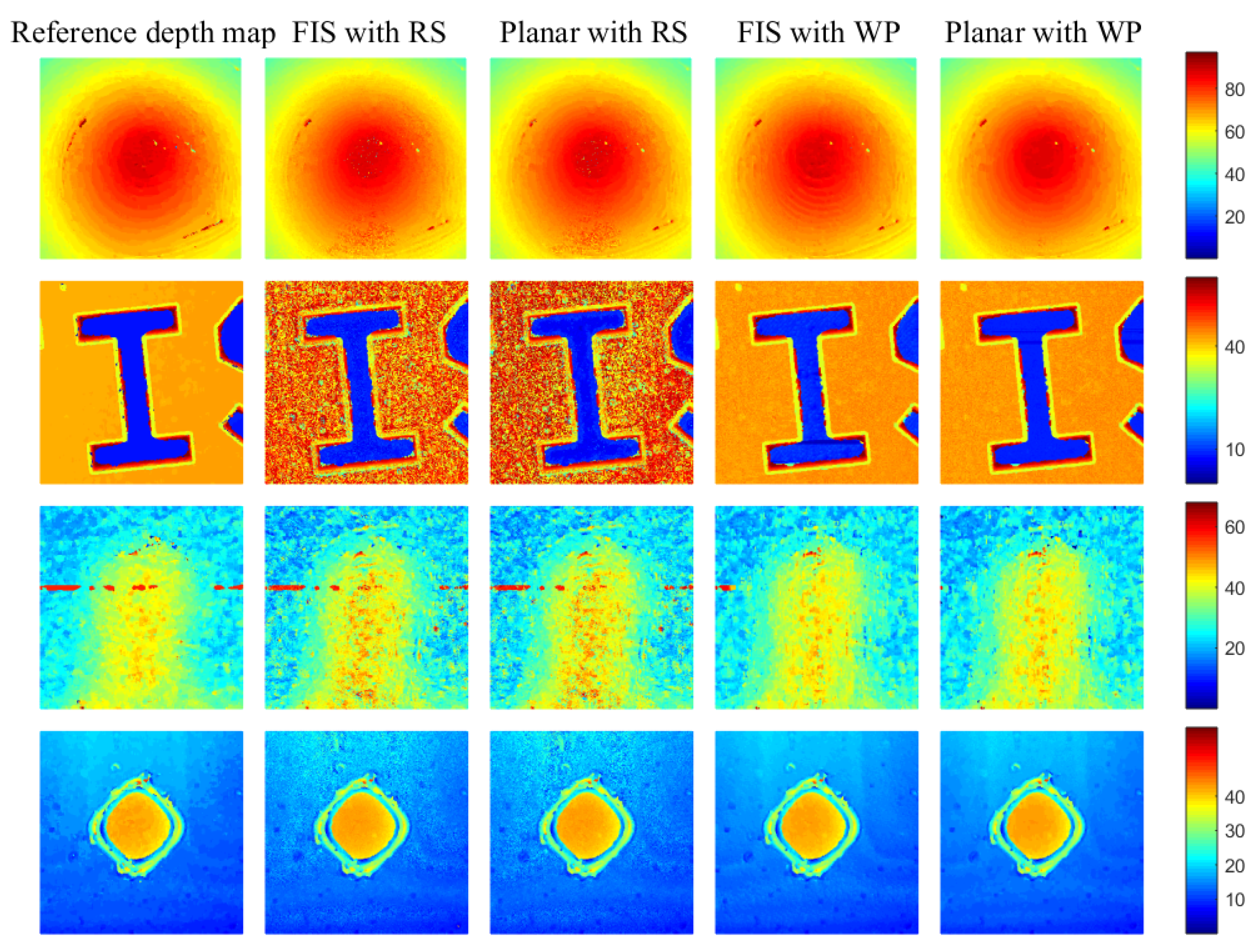
5.3. Qualitative Analysis

Figure 8 shows restored 3D depth maps for synthetic objects with different learning iterations. At first or second column, when total iteration is 1 or 5, the network produces inaccurate results at pixel positions having high reference depth. The reason is that it needs sufficient iteration to converge the depth at the previous pixel of inaccuracy. Therefore, it needs a sufficient total iteration number, over 50 iterations in our simulation, to ensure depth convergence for all pixels. In addition, note that we can roughly acquire the restored depth map, appearing to be the corresponding object, even 1 iteration. That is the strength of WP method. Specifically, when the total iteration is not enough, depths at the first few pixels (its pixel positions having low reference depth) are considerably precise; however, depths return to be distorted after some pixels (its pixel positions having high reference depth). In addition, overall depth map can be precisely restored at 50 iterations, which is also smaller iterations than other usual neural networks.

Resultant depth maps for various SFF methods using synthetic objects are show in Figure 9. From the figure, it is clear that (1) the precision of restored depth map by using NN.FIS or NN.Planar is almost similar to each other with a same initial weight setting. It means that the NN.Planar model is more efficient than the NN.FIS model because it gives similar performance with less complexity; And (2) WP initial setting method facilitates more precise restoring than RS when using a same neural network model. Specifically, the Planer and Sinusoidal objects include pixel positions having high depth near to the maximum depth. In the pixel positions, it is hard to estimate a depth precisely with RS method because of short of iteration, thus it affects the precision of entire restored depth map. However, WP relieves the problem regardless of the histogram of depth. In addition, Figure 10 shows the restored 3D depth map by using real objects. Similarly, NN.FIS and NN.Planar with a same initial weight setting method give almost same restored depth. In addition, WP gives more precise restored depth map than RS in a same neural network model. The reference depth map is utilized as a reference for generating an initial depth map. In the case of coin object, the restored depth map by SML is used as the reference map for coin object. In addition, other objects utilize the restored depth map by GLV as the reference map for the objects. Note that the reference depth map of each object contains several errors, but the errors are reduced by using Planar with WP. In addition the errors increase slightly or heavily with an object by using Planar with RS, because the RS method needs enough iteration larger than 50. In order to solve the errors in RS, the total iteration number should be increased enough but it gives time complexity.

6. Discussion

The presented method is one of the paradigms of 3D shape recovery techniques known as SFF. Three-dimensional shapes have possible potentials for various applications including motion reconstruction [30,31,32], 3D object retrieval [33], 3D cameras, manufacture of TFT-LCD color filter, and measurement of surface roughness, medical examinations, microelectronics, and focus variation for 3D surface. The proposed method is a simplified version of the previous well-known methods based on neural network. From the experimental results, it is clear that the proposed model has considerably reduced the complexity without a loss in accuracy. It is expected that if the PCA is used to reduce the dimensionality to select the surface locally, it can give marginally better accurate depth than the NN.Planar. However, the additional computational complexity by PCA will rise proportional to the total iteration numbers. It would be interesting to do a separate study that can make fair comparisons among the methods based on different dimensionality reduction techniques for three shape refinement through the SFF in term of complexity and accuracy.

In literature, a number of machine learning techniques such as convolutional neural network (CNN) [34,35], deep convolutional neural network (DCNN) [36,37] recurrent neural network (RNN) [38], graphical model [39], have been proposed. Among these, CNN includes the fully connected layers which connect each neuron in a layer to all neurons in the next layer. It is similar to the feedforward artificial neural network. Therefore, WP method can be applied with the same settings by using CNN for 3D imaging applications to reduce local minimization. Similarly, the other well-known techniques are also applicable with modifications in the weight update procedures.

In machine learning techniques, the restricted Boltzmann machine [24,25,26] are considered powerful methods to pre-process the input data to expedite the learning process. In our future work, the restricted Boltzmann machines will be used, instead of reducing the dimensionality of the data, in refining the depth maps in SFF. It is expected that RBM will provide depth maps efficiently with higher accuracy. In addition, it would be interesting to do a separate study for comparing the performances of different machine learning-based methods in 3D shape recovery in SFF in terms of efficacy and accuracy.

7. Conclusions

In this paper, a simplified neural network over planar model is proposed for SFF. In addition, for rapid convergence and efficiency of the network, WP method has been introduced. The simplified neural network model takes input and weight vector of smaller size, and the WP method selects proper initial weights for the first pixel randomly and it updates the initial weights for the next pixel efficiently by passing the updated weight from the present pixel. The proposed method significantly has reduced the computational complexity while the accuracy is comparable with the conventional model.

8. Patents

There is a patent [40] resulting from the work reported in this manuscript.

References

1. Lee, I.H.; Mahmood, M.T.; Choi, T.S. Robust Depth Estimation and Image Fusion Based on Optimal Area Selection. Sensors 2013, 13, 11636–11652. [Google Scholar] [CrossRef] [PubMed] [Green Version]
2. Ahmad, M.; Choi, T.S. Application of Three Dimensional Shape from Image Focus in LCD/TFT Displays Manufacturing. IEEE Trans. Consum. Electron. 2007, 53, 1–4. [Google Scholar] [CrossRef]
3. Mahmood, M. MRT letter: Guided filtering of image focus volume for 3D shape recovery of microscopic objects. Microsc. Res. Tech. 2014, 77, 959–963. [Google Scholar] [CrossRef] [PubMed]
4. Mahmood, M.; Choi, T.S. Nonlinear Approach for Enhancement of Image Focus Volume in Shape from Focus. IEEE Trans. Image Process. 2012, 21, 2866–2873. [Google Scholar] [CrossRef] [PubMed]
5. Thelen, A.; Frey, S.; Hirsch, S.; Hering, P. Improvements in Shape-From-Focus for Holographic Reconstructions with Regard to Focus Operators, Neighborhood-Size, and Height Value Interpolation. IEEE Trans. Image Process. 2009, 18, 151–157. [Google Scholar] [CrossRef] [PubMed]
6. Tang, H.; Cohen, S.; Price, B.; Schiller, S.; Kutulakos, K.N. Depth from Defocus in the Wild. In Proceedings of the 2017 IEEE Conference on Computer Vision and Pattern Recognition (CVPR), Honolulu, HI, USA, 21–26 July 2017; pp. 4773–4781. [Google Scholar] [CrossRef]
7. Frommer, Y.; Ben-Ari, R.; Kiryati, N. Shape from Focus with Adaptive Focus Measure and High Order Derivatives. In Proceedings of the British Machine Vision Conference (BMVC), Swansea, UK, 7–10 September 2015; p. 134. [Google Scholar] [CrossRef]
8. Suwajanakorn, S.; Hernandez, C.; Seitz, S.M. Depth from focus with your mobile phone. In Proceedings of the 2015 IEEE Conference on Computer Vision and Pattern Recognition (CVPR), Boston, MA, USA, 7–12 June 2015; pp. 3497–3506. [Google Scholar] [CrossRef]
9. Bishop, C.M. Pattern Recognition and Machine Learning; Springer: New York, NY, USA, 2006; Available online: https://www.springer.com/us/book/9780387310732 (accessed on 13 September 2018).
10. Asif, M.; Choi, T.S. Shape from focus using multilayer feedforward neural networks. IEEE Trans. Image Process. 2001, 10, 1670–1675. [Google Scholar] [CrossRef] [PubMed] [Green Version]
11. Malik, A.S.; Choi, T.S. Consideration of illumination effects and optimization of window size for accurate calculation of depth map for 3D shape recovery. Pattern Recognit. 2007, 40, 154–170. [Google Scholar] [CrossRef]
12. Pertuz, S.; Puig, D.; Garcia, M.A. Analysis of focus measure operators for shape-from-focus. Pattern Recognit. 2013, 46, 1415–1432. [Google Scholar] [CrossRef]
13. Huang, W.; Jing, Z. Evaluation of focus measures in multi-focus image fusion. Pattern Recognit. Lett. 2007, 28, 493–500. [Google Scholar] [CrossRef]
14. Ahmad, M.; Choi, T.S. A heuristic approach for finding best focused shape. IEEE Trans. Circuits Syst. Video Technol. 2005, 15, 566–574. [Google Scholar] [CrossRef]
15. Boshtayeva, M.; Hafner, D.; Weickert, J. A focus fusion framework with anisotropic depth map smoothing. Pattern Recognit. 2015, 48, 3310–3323. [Google Scholar] [CrossRef] [Green Version]
16. Hariharan, R.; Rajagopalan, A. Shape-From-Focus by Tensor Voting. IEEE Trans. Image Process. 2012, 21, 3323–3328. [Google Scholar] [CrossRef] [PubMed]
17. Tseng, C.Y.; Wang, S.J. Shape-From-Focus Depth Reconstruction with a Spatial Consistency Model. IEEE Trans. Circuits Syst. Video Technol. 2014, 24, 2063–2076. [Google Scholar] [CrossRef]
18. Tenenbaum, J.B.; de Silva, V.; Langford, J.C. A Global Geometric Framework for Nonlinear Dimensionality Reduction. Science 2000, 290, 2319–2323. [Google Scholar] [CrossRef] [PubMed]
19. Shlens, J. A Tutorial on Principal Component Analysis. arXiv, 2014; arXiv:1404.1100. [Google Scholar]
20. Borg, I.; Groenen, P.J.; Mair, P. Applied Multidimensional Scaling and Unfolding, 2nd ed.; Springer: New York, NY, USA, 2018; Available online: https://www.springer.com/gb/book/9783319734705 (accessed on 13 September 2018).
21. Cao, L.; Chua, K.; Chong, W.; Lee, H.; Gu, Q. A comparison of PCA, KPCA and ICA for dimensionality reduction in support vector machine. Neurocomputing 2003, 55, 321–336. [Google Scholar] [CrossRef]
22. Roweis, S.T.; Saul, L.K. Nonlinear Dimensionality Reduction by Locally Linear Embedding. Science 2000, 290, 2323–2326. [Google Scholar] [CrossRef] [PubMed] [Green Version]
23. Belkin, M.; Niyogi, P. Laplacian Eigenmaps for Dimensionality Reduction and Data Representation. Neural Comput. 2003, 15, 1373–1396. [Google Scholar] [CrossRef] [Green Version]
24. Ngiam, J.; Khosla, A.; Kim, M.; Nam, J.; Lee, H.; Ng, A.Y. Multimodal Deep Learning. In Proceedings of the 28th International Conference on International Conference on Machine Learning (ICML’11), Bellevue, WA, USA, 28 June–2 July 2011; Omnipress: Madison, WI, USA, 2011; pp. 689–696. [Google Scholar]
25. Mousas, C.; Anagnostopoulos, C.N. Learning Motion Features for Example-Based Finger Motion Estimation for Virtual Characters. 3D Res. 2017, 8, 25. [Google Scholar] [CrossRef]
26. Nam, J.; Herrera, J.; Slaney, M.; Smith, J. Learning Sparse Feature Representations for Music Annotation and Retrieval. In Proceedings of the 2012 International Society for Music Information Retrieval (ISMIR), Porto, Portugal, 8–12 October 2012; pp. 565–570. [Google Scholar]
27. Asif, M. Shape from Focus Using Multilayer Feedforward Neural Networks. Master’s Thesis, Gwangju Institute of Science and Technology, Gwangju, Korea, 1999. [Google Scholar]
28. Pertuz, S. Defocus Simulation. Available online: https://kr.mathworks.com/matlabcentral/fileexchange/55095-defocus-simulation (accessed on 12 September 2018).
29. Favaro, P.; Soatto, S.; Burger, M.; Osher, S.J. Shape from Defocus via Diffusion. IEEE Trans. Pattern Anal. Mach. Intell. 2008, 30, 518–531. [Google Scholar] [CrossRef] [PubMed]
30. Holden, D.; Komura, T.; Saito, J. Phase-functioned Neural Networks for Character Control. ACM Trans. Graph. 2017, 36, 42. [Google Scholar] [CrossRef]
31. Mousas, C.; Newbury, P.; Anagnostopoulos, C.N. Evaluating the Covariance Matrix Constraints for Data-driven Statistical Human Motion Reconstruction. In Proceedings of the 30th Spring Conference on Computer Graphics (SCCG’14), Smolenice, Slovakia, 28–30 May 2014; ACM: New York, NY, USA, 2014; pp. 99–106. [Google Scholar] [CrossRef]
32. Mousas, C.; Newbury, P.; Anagnostopoulos, C.N. Data-Driven Motion Reconstruction Using Local Regression Models. In Artificial Intelligence Applications and Innovations, Proceedings of the 10th IFIP International Conference on Artificial Intelligence Applications and Innovations (AIAI), Rhodes, Greece, September 2014; Iliadis, L., Maglogiannis, I., Papadopoulos, H., Eds.; Part 8: Image—Video Processing; Springer: Berlin/Heidelberg, Germany, 2014; Volume AICT-436, pp. 364–374. Available online: https://hal.inria.fr/IFIP-AICT-436/hal-01391338 (accessed on 13 September 2018). [CrossRef]
33. Krizhevsky, A.; Sutskever, I.; Hinton, G.E. Imagenet classification with deep convolutional neural networks. In Proceedings of the 25th International Conference on Neural Information Processing Systems, Lake Tahoe, Nevada, USA, 3–6 December 2012; pp. 1097–1105. [Google Scholar]
34. Cheron, G.; Laptev, I.; Schmid, C. P-CNN: Pose-based CNN Features for Action Recognition. arXiv, 2015; arXiv:1506.03607. [Google Scholar]
35. Abdel-Hamid, O.; Mohamed, A.R.; Jiang, H.; Penn, G. Applying convolutional neural networks concepts to hybrid NN-HMM model for speech recognition. In Proceedings of the 2012 IEEE International Conference on Acoustics, Speech and Signal Processing (ICASSP), Kyoto, Japan, 25–30 March 2012; pp. 4277–4280. [Google Scholar]
36. Saito, S.; Wei, L.; Hu, L.; Nagano, K.; Li, H. Photorealistic Facial Texture Inference Using Deep Neural Networks. arXiv, 2016; arXiv:1612.00523. [Google Scholar]
37. Li, R.; Si, D.; Zeng, T.; Ji, S.; He, J. Deep Convolutional Neural Networks for Detecting Secondary Structures in Protein Density Maps from Cryo-Electron Microscopy. In Proceedings of the IEEE International Conference on Bioinformatics and Biomedicine, Shenzhen, China, 15–18 December 2016; pp. 41–46. [Google Scholar]
38. Li, Z.; Zhou, Y.; Xiao, S.; He, C.; Li, H. Auto-Conditioned LSTM Network for Extended Complex Human Motion Synthesis. arXiv, 2017; arXiv:1707.05363. [Google Scholar]
39. Bilmes, J.; Bartels, C. Graphical model architectures for speech recognition. IEEE Signal Process Mag. 2005, 22, 89–100. [Google Scholar] [CrossRef]
40. Kim, H.J.; Mahmood, M.T.; Choi, T.S. A Method for Reconstruction 3-D Shapes Using Neural Netwok. Korea Patent 1,018,166,630,000, 2018. Available online: https://doi.org/10.8080/1020160136767 (accessed on 9 January 2018).
Figure 1. Principle of image sequence acquisition in shape from focus (SFF).
Applsci 08 01648 g001
Figure 2. Multilayer feedforward neural network structure for shape recovery of neural network model over FIS and local depth map from the neural network model. Left: NN.FIS model; Right: local depth map from NN.FIS model. The local depth map consists of 9 neighboring pixels centered around ( x , y ) , when small window size is 3 × 3 . In addition, each local depth is produced by network with changing the local index j and k.
Applsci 08 01648 g002
Figure 3. Proposed neural network structure for shape recovery of neural network model over Planar and local depth map from the neural network model. Left: NN.Planar model; Right: local depth map from NN. Planar model. The local depth map consists of 9 neighboring pixels centered around ( x , y ) , when small window size is 3 × 3 . In addition, all local depths are same to the depth at center, so it can reduce the dimension of input layer from 3 to 1.
Applsci 08 01648 g003
Figure 4. Histogram of z ( x , y ) ( 1 ) values. It graphically represents the distribution of numerical data of z ( x , y ) ( 1 ) . In addition, the bins are same size of 0.01 and the total frequency is 10,000. Note that it is similar to the Gaussian distribution, and thus the frequency number is very low at a range of z ( x , y ) ( 1 ) 0.1 or z ( x , y ) ( 1 ) 0.9 . Consequently, in the range, it is hard to meet the requirements of | z ( x , y ) ( 1 ) z r ( x , y ) | T 1 within R, and thus it fails to set the proper initial weights in RS method.
Applsci 08 01648 g004
Figure 5. The proposed WP initial weight setting method. (a) z r ( x , y ) is a reference depth map estimated by Sum-Modified-Laplacian (SML) or Gray-Level-Variance (GLV); (b) z r ( s ) is 1-dimensional vector form of the z r ( x , y ) and s is the index of z r ( s ) ; (c) z ^ r ( t ) is the sorted reference depth map into depth order, t is the index of z ^ r ( t ) , s ^ ( t ) is the index of z r ( s ) corresponding to the depth of z ^ r ( t ) , and ( x ^ ( t ) , y ^ ( t ) ) is the index of z r ( x , y ) corresponding to the depth of z ^ r ( t ) .
Applsci 08 01648 g005
Figure 6. (a) Sample frames from image sequences of synthetic objects: plane object (first row), sinusoidal object (second row), cone object (third row), and wave object (fourth row). In addition, each column shows frame number 20, frame number 40, and frame number 70. In a sample frame, the texture clearly distinguishes only at the well focused area; (b) Sample frames from image sequences of real objects: real cone (first row), engraved letter I (second row), coin (third row), and TFT-LCD color filter (fourth row). In a sample frame, the texture clearly distinguishes only at the well focused area.
Applsci 08 01648 g006
Figure 7. Box plot of the normalized Root-Mean-Square-Error (RMSE) from 30 experiments for Planar with WP and Planar with RS using various objects.
Applsci 08 01648 g007
Figure 8. Restored three-dimensional (3D) depth maps for synthetic objects with different learning iterations, first row: plane object, second row: sinusoidal object, third row: cone object, and fourth row: wave object. In addition, first column: Iteration 1, second column: Iteration 5, and third column: Iteration 50. In this experiment, the Planar model with WP method is utilized for measuring depth map.
Applsci 08 01648 g008
Figure 9. Restored 3D depth map for various SFF methods using various synthetic objects, first row: plane object, second row: sinusoidal object, third row: cone object, and fourth row: wave object. In addition, first column: True depth map, second column: NN.FIS with RS, third column: NN.Planar with RS, fourth column: NN.FIS with WP, and fifth column: NN.Planar with WP.
Applsci 08 01648 g009
Figure 10. Restored 3D depth map for various SFF methods using various real objects, first row: real cone object, second row: engraved I object, third row: coin object, and fourth row: TFT-LCD filter object. In addition, first column: True depth map, second column: NN.FIS with RS, third column: NN.Planar with RS, fourth column: NN.FIS with WP, and fifth column: NN.Planar with WP.
Applsci 08 01648 g010